Sage Journals: Discover world-class research

Abstract

This work investigates the strength of artificial neural network that is trained by an optimization technique called particle swarm optimization in the task of time series prediction of weekly and monthly significant wave heights. The suggested approach has been implemented at the location of New Mangalore Port in India. Three years of wave data measured during 2005–2007 are analyzed. It is found that the network trained with the help of the particle swarm optimization produces more accurate predictions of the significant wave heights and further with lesser amount of data than the traditionally trained feed-forward back-propagation network.

Keywords

Artificial neural network feed-forward back-propagation particle swarm optimization Levenberg–Marquardt algorithm

Introduction

Information on wave heights at a site is required for design- as well as operation-related activities in the ocean. Forecasting of waves for operational or design purpose can be made by measuring and analyzing the actual wave observations at a given location. But considering the difficulties and costs involved in getting large-scale wave data, many times, the readily available wind information is gathered and then converted into corresponding wave information although this procedure is less accurate than the actual wave analysis.

A new model based on the working of human brain has been idealized to meet the objective of learning relationship between complex parameters involved in the interaction without having to know the underlying physics behind it. As it is an attempt to mimic the capabilities of the human neural system, it is called artificial neural network (ANN). It imbibes the qualities of exploiting non-linearity—adaptability to adjust free parameters by mapping input output data sets using various learning algorithms and fault tolerance.

A considerable amount of literature dealing with the use of ANN for wave forecasting is available. After McCulloch and Pitts (1943) introduced the concept of a basic ANN, many advanced architectures were presented. Among those models, the multi-layered network trained by back-propagation (BP) algorithm has been applied extensively to solve various engineering problems.

Tsai and Lee (1999) reported an application of the feed-forward neural network to forecast the wave heights at a given site based on the observed wave data of some other site within the Taichung Harbor. Results showed that the wave forecast at a local site has a better performance when the wave data of multisite observations are used.

The most common training algorithm is the standard BP, although numerous training schemes are available to impart better training with the same set of data as shown by Londhe and Deo (2003) in their harbor tranquility studies.

The work carried out by Rao and Mandal (2005) describes hind-casting of wave heights and periods from cyclone-generated wind fields using two-input configurations of ANN. They use advanced algorithms based on the BP neural network due to which the wave forecasting was better.

Deo and Sridhar Naidu (1999) described the application of ANNs in forecasting significant wave heights with a 3-hour lead period. They carried out different combinations of training patterns to obtain the desired output and used three different algorithms of BP, conjugate gradient descent, and cascade correlation to predict wave height.

Tsai et al. (2002) used BP ANN to forecast the ocean waves based on learning characteristics of observed waves and also based on wave records at the neighboring stations.

A comprehensive review of ANN applications in ocean engineering can be seen in Jain and Deo (2006). They pointed out that ANN can provide a good alternative to statistical regression, time series analysis and numerical methods. There are many comparison studies to find out the appropriate method for prediction. Altunkaynak and Ozger (2004) have performed a comparison between perceptron kalman filtering and classical regression for significant wave height and wind speed measurement from USA in the Coos Bay at Oregon. The results have shown that the PKF approach is better than the classical RM procedures. Wave forecasting was done using wind velocity, fetch and duration as input parameters (Deo and Chaphekar, 2001). The results were not satisfactory – fetch and duration were excluded as their presence did not have any effect on predictions. Deo and Jagdale (2003) carried out a study to predict the breaking wave height and depth using five different datasets. The results obtained were found to be better than those obtained by regression curves given by the US Army (1984). Balas et al (2004) used multilayered feed forward and recurrent networks with conjugate gradient and steepest descent with momentum method to predict wave parameters of significant wave height, zero crossing wave period, and wave direction. They compared the results with those obtained from stochastic models of Auto Regressive and Auto Regressive eXogenous input models. Mahjoobi and Shahidi (2008) employed feed forward network with three layers using the sigmoid and hyperbolic tangent function. Three models were created for each output of wave direction, significant wave height and peak wave period. Sensitivity analysis showed that wind speed and direction is the most important parameter for wave hind casting. They excluded fetch and duration in their work and developed an ANN model. Their results confirm that these two parameters do not play an important role in the model’s accuracy. Similar results were obtained by Deo et al (2001) and Deo (2010). They concluded that, unlike the deterministic models, fetch and duration do not seem to be important in ANN modeling. This fact can be generalized when we are using any kind of data mining approach (Mahjoobi et. al, 2008).

Jain and Deo (2007) also used the ANN for wave forecasting. They found that filling the gaps in the wave height time series, using both temporal and spatial approaches, improves the learning capability of the model. They also indicated that if the amount of gaps is restricted to about 2% per year or so, it is possible to obtain 12 h ahead forecasts with 0.08 m accuracy and 24 h ahead forecast with a mean accuracy of 0.13 m. Agrawal and Deo (2004) also used ANN and auto regressive models, i.e. ARMA (Auto Regressive Moving Average) and ARIMA (Auto Regressive Integrated Moving Average) for wave prediction. They used a 3-hourly significant wave height information as input and compared three training algorithms to find the best one. They found that ANN has higher accuracy than the auto regressive methods for 3 and 6 h lead times. Zamani et al. (2008) forecasted wave height in the Caspian Sea using ANN and Instance Based Learning (IBL) methods. They used Average Mutual Information analysis to determine the most relevant inputs of the model. They considered wind direction in their models and showed that the accuracy of ANN is more than that of IBL. They also found that the utilization of ANN in prediction of extreme values yields higher accuracy compared to the utilization of IBL. Several researchers have already worked on applications related to ANN in the areas of estimation of wave parameters, tide prediction, and prediction of short term operational water levels (Deo and Naidu, 1999); Rao et al., 2001; Tsai et al., 2002; Deo and Jagdale, 2003; Balas et al., 2004; Kalra et al., 2005; Makarynskyy et al., 2005; Mandal et al., 2008; Rao and Mandal, 2005; Londhe and Panchang, 2006; Londhe SN, 2008’ Mandal and Prabhaharan, 2006; Jain and Deo, 2007); Kalra and Deo, 2007; Charhate et al., 2008; Gunaydin, 2008; Londhe, 2008 Mahjoobi and Etemad -Shahidi, 2008; Mahjoobi et al., 2008; Zamani et al., 2008; Mandal and Prabhaharan, 2010; Kamranzad et al., 2011; Shiri et al., 2011; Asma et al., 2012; Rakshith and Dwarakish, 2013; Kamranzad et al, 2011; Kennedy and Eberhart, 1995.

Study area and data products

Three years of significant wave height data collected by a wave rider buoy from January 2005 to December 2007 at the location of New Mangalore Port (14°48′34.28″N, 74°07′02.85″E) were utilized in this study. The location map of study area is shown in Figure 1. Predictions were carried out using a week’s data of 56 time steps (8 hour × 7 days) and month’s data of 240 time steps (8 hour × 30 days) as input.

Figure 1.

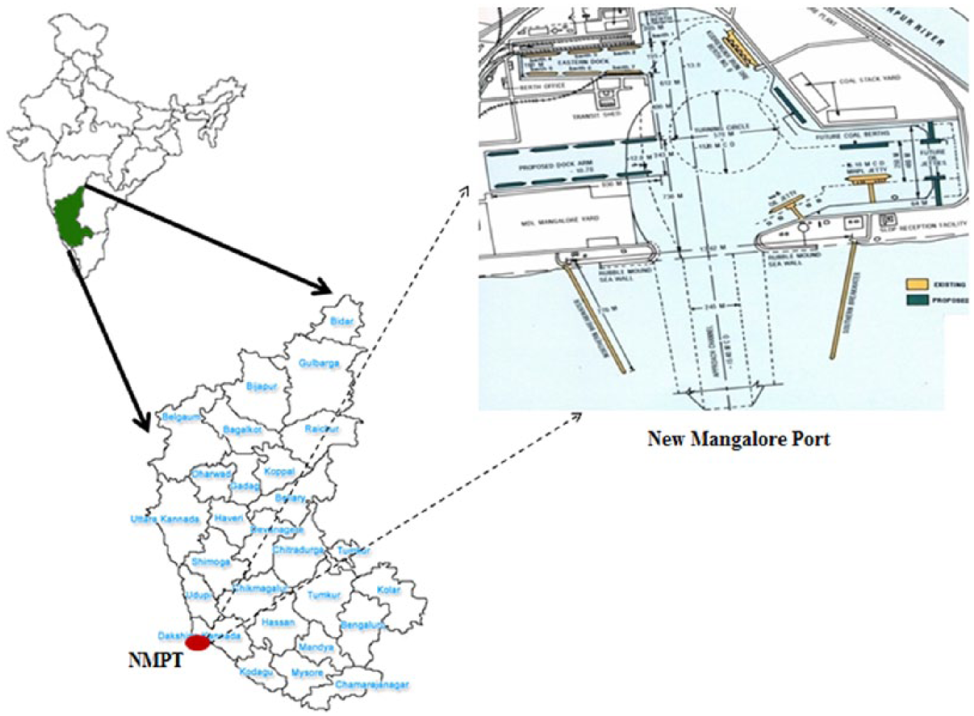
Location map of study area.

A three-layered feed-forward back-propagation (FFBP) network with an input layer, a hidden layer, and an output layer with training imparted by the Levenberg–Marquardt (LM) algorithm was employed. Tangent-Sigmoid (tansig) and linear (purelin) transfer functions were used in hidden layer and output layer, respectively. The data were normalized to fall in the range of −1 to 1 to speed up the learning process. In total, 1000 were set as the stopping criterion for the training process of network for all the predictions undertaken.

Methodology

FFBP network

ANNs are computing systems made up of simple, interconnected elements, which process information by their response to external inputs. The ANNs have developed from a biological model of the brain. A neural network consists of a set of connected cells or neurons. The neurons receive impulses from either input cells or other neurons and perform some kind of transformation of the input and transmit the outcome to other neurons or to output cells. The neural networks are built from layers of neurons connected so that one layer receives input from the preceding layer of neurons and passes the output on to the subsequent layer.

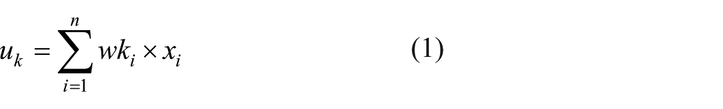
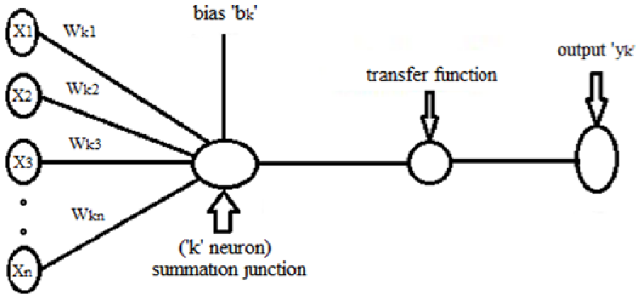
A graphical presentation of neuron is given in Figure 2. A neuron is a real function of the input vector x₁, x₂, x₃, … x_n and wk₁, wk₂, wk₃, … wk_n are the weights associated with it. Neuron k is the summation junction where the net input obtained is given by

u_{k} = \sum_{i = 1}^{n} w k_{i} \times x_{i}

(1)

v_{k} = u_{k} + b_{k}

(2)

b_k is the bias value at the kth neuron. The output Y_k is the transformed weighted sum of v_k and is represented by

Y_{k} = ϕ (v_{k})

(3)

where $ϕ$ is the transfer function or activation function used to convert the summed input. A non-linear sigmoid function which is monotonically increasing and continuously differentiable is the most commonly used activation function. It can be mathematically expressed as

Y_{k} = ϕ (v_{k}) = \frac{1}{[1 + \exp (- a v_{k})]}

(4)

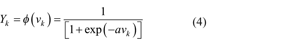
where a is the slope of sigmoid function. Once the activities of all output units have been determined, the network computes the error E, which is defined by the expression

E = \frac{1}{2} \times \sum_{i = 1}^{n} {(y_{i} - d_{i})}^{2}

(5)

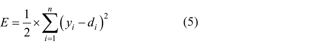
where y_i is the activity level of the ith unit in the top layer and d_i is the desired output of the ith unit. The most commonly used learning algorithm in the past coastal engineering applications is the gradient descent algorithm. In this, the computed global error is propagated backward to the input layer through weight connections, during which the weights are updated in the direction of the steepest descent or in the direction opposite to the gradient descent. However, the overall objective of any learning algorithm is to reduce the global error, E, defined as

E = \frac{1}{p} \sum_{p = 1}^{p} E_{p}

(6)

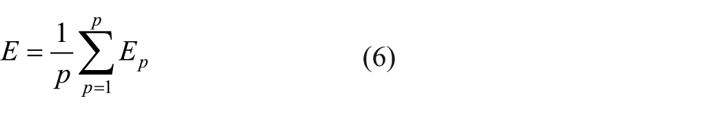
and

E_{p} = \frac{1}{2} \sum_{k = 1}^{N} {(O_{k} - t_{k})}^{2}

(7)

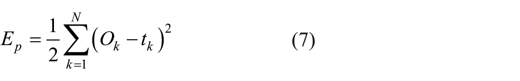
where E_p is the error at the pth training pattern, O_k is the obtained output from network at the kth output node, t_k is the target output at the kth output node, and N is the total number of output nodes. The training algorithm of LM used in this study can be written as

W_{new} = W_{old} {[J^{T} J + γ I]}^{- 1} J^{T} E (W_{old})

(8)

where J is the Jacobian of the error function (E), I is the identity matrix, and γ is the parameter used to define the iteration step value. It minimizes the error function while trying to keep the step between old weight configuration (W_old) and new updated one (W_new) small.

Figure 2.

Basic model of ANN.

The performance of the network is measured in terms of various error statistics such as the sum squared error (SSE), mean squared error (MSE), root mean squared error (RMSE), and coefficient of correlation (r) between the predicted and the observed values of the quantities. A low value of RMSE and high value of CC indicate better performance of the network. The major drawback of the FFBP is that of the network getting trapped in the local minima. Too many variations in the involved data set will diminish the accuracy of the network. The mentioned setbacks can, however, be overcome by selecting the optimum architecture of the network using various techniques like sensitivity analysis to select most effective input parameters and reduce network size to decrease the computational time required.

Particle swarm optimization–ANN network

The particle swarm optimization (PSO) is an optimization algorithm first proposed by Kennedy and Eberhart (1995). PSO is based on swarm intelligence, such as the behavior of swarms of bees seeking out flowers to pollinate. The swarm is composed of particles, where each particle represents a possible solution to an optimization problem. PSO is initialized with a group of random particles (solutions), which were assigned with random positions and velocities. The algorithm then searches for optima through a series of iterations where the particles are flown through the hyperspace searching for potential solutions. These particles learn over time in response to their own experience and other particles’ experience in their group. Each particle keeps track of its best fitness position in hyperspace that it has achieved so far. This best position value is called personal best or “pbest.” The overall best value obtained by any particle so far in the population is called global best or “gbest.” During iteration, every particle is accelerated toward its own “pbest” as well as in the direction of the “gbest” position. This is achieved by calculating a new velocity term for each particle based on the distance from its “pbest” as well as its distance from the “gbest” position. These two “pbest” and “gbest” velocities are then randomly weighted to produce the new velocity value for this particle, which will affect the next position of the particle in next iteration.

The advantage of the PSO over many of the optimization algorithms is its relative simplicity. The only two equations used in PSO are the movement equation and velocity update equation. The movement equation provides for the actual movement of the particles using their specific vector velocity, while the velocity updates equation provides for velocity vector adjustment given the two competing forces. Besides, inertia weight (w) is introduced to improve the convergence rate of the PSO algorithm. Mathematically

p r e s L o c a t i o n = p r e v L o c a t i o n + V_{i} Δ t

(9)

V_{i} = w V_{i - 1} + c_{1} \times r a n d () \times (p b e s t - p r e s L o c a t i o n) + c_{2} \times r a n d () \times (g b e s t - p r e s L o c a t i o n)

(10)

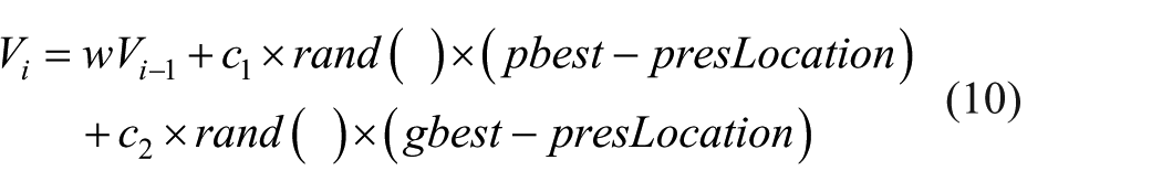
where V_i is the current velocity, Δt defines the discrete time interval over which the particle will move, w is the inertia weight, V_i₋₁ is the previous velocity, presLocation is the present location of the particle, prevLocation is the previous location of the particle, rand () is a random number between (0, 1), and c₁ and c₂ are the learning factors or stochastic factors or acceleration constants for “gbset” and “pbest,” respectively.

Results and discussion

Prediction using FFBP network

Weekly predictions

In this study, the prediction over a horizon of 4 weeks was carried out using 1 week’s wave data from 1 January 2005 to 7 January 2005 as input. The target data set comprised readings of 4 weeks’ duration from 8 January 2005 to 4 February 2005 (28 days), 1 week’s data having 56 time steps (8 hours × 7 days) representing a single node in this case which is represented as row matrix (1 × 56), and similarly an output layer consisting of four nodes for 4 weeks of data. Subsequent weeks in similar fashion were given as input and target for testing the trained network. The “r” values showed marginal increase in 4-week prediction which might be due to the increased number of target values available for the network generalization. However, the “r” value decreased for the 12-week wave prediction as 1 week’s data range is too small for predicting a long duration of 12-week wave data. The number of neurons was increased in the hidden layer by one, after every prediction. The best performance was obtained at six and four neurons in the hidden layer during 4- and 12-week prediction of wave height as shown in Table 1. The training performance showed that considerable increase in “r” values drastically reduced hinting at the overfitting behavior of the network when the number of neurons was increased beyond six and four during 4- and 12-week wave prediction. This phenomenon refers to a state where there is a large number of neurons in hidden layer increasing the complexity of the network, but there is no significant amount of patterns to be learnt by the network based on given input-target data sets. Also in both the cases, the prediction duration is large compared to input data. Naturally, the range of targets will be greater than those of input provided, weakening the prediction capability of the network when new data set is fed to the network.

Table 1.

Root mean square error (“RMSE”) and correlation coefficient (“r”) values for wave predictions of 4, 12, and 52 weeks.

Network architecture	RMSE		r
Network architecture	Training	Testing	Training	Testing
1-6-4	0.13	1.503	0.811	0.755
1-4-12	0.167	3.05	0.775	0.65
52-10-52	0.144	0.835	0.994	0.918

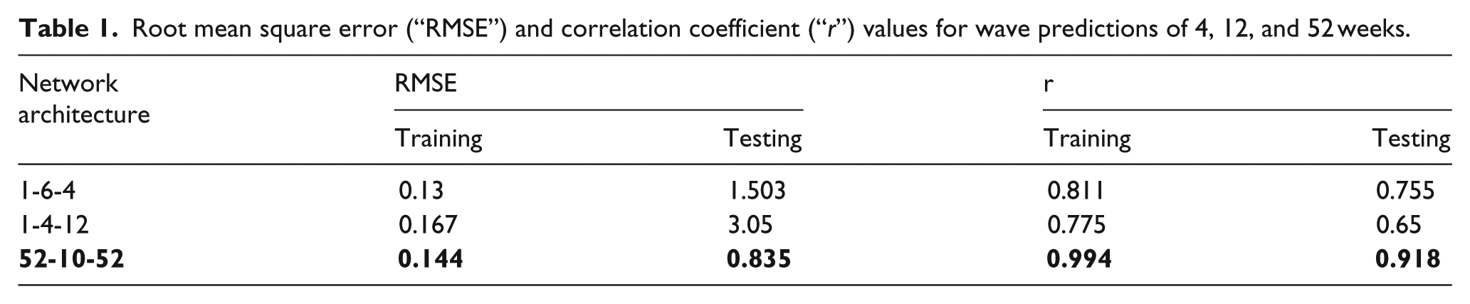
Similarly, yearlong predictions are carried out using data of year 2005 as input and data of year 2006 as target in the training process and next two consecutive year’s data (2006 and 2007) as input and target for simulation purpose, respectively. The input and output layers consisted of 52 nodes representing 52-week data for a single year. The prediction done using yearlong data yielded good results with training process “r” value reaching up to 0.99 and simulation “r” value reaching a value of 0.91. The optimum number of neurons is found to be 10 and the “MSE” values are 0.021 and 0.698 for training and simulation purpose, respectively. The increase in the number of neurons beyond 10 led to a decrease in the prediction capability of the trained network when simulation data sets are presented to the network. The plot of observed values and predicted values shown in the Figures 3 and 4 gives the scatter plot of training and simulation of the network.

Figure 3.

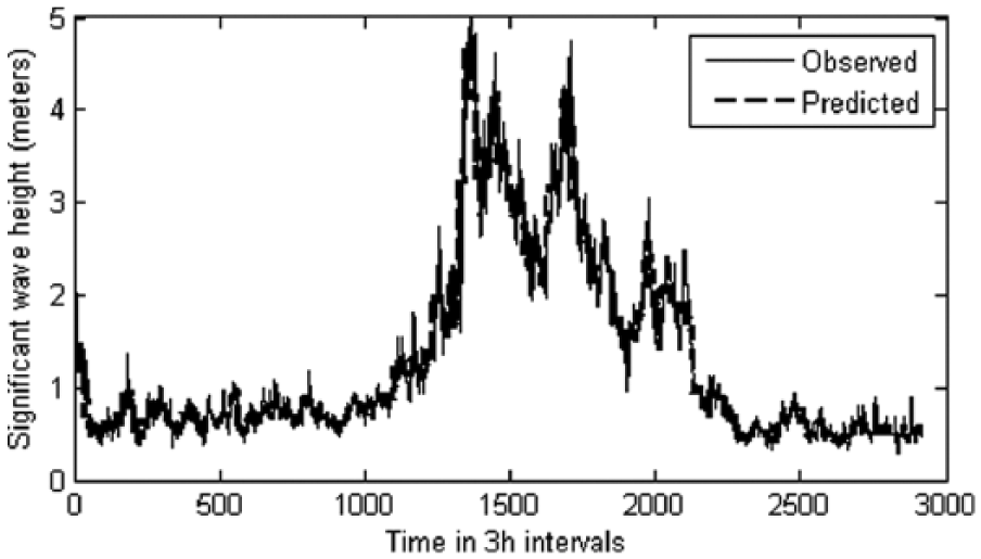
Graph showing the predicted and observed waves for the year 2006 using weekly data sets (1 January 2005 to 30 December 2005) in the FFBP network.

Figure 4.

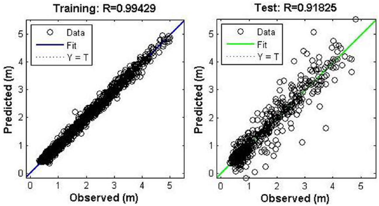
The scatter plot of training and simulation of the network during yearly predictions done using weekly data sets in the FFBP network.

Monthly predictions

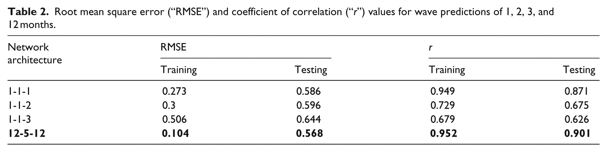
Monthly prediction involved feeding the network with 1 month’s data having 240 data points in a single input node (1 × 240). The year 2005 hourly wave data are divided into 12 sets having 240 data points, each corresponding to 30 days of observation; hence, the yearly data comprised 1 January 2005 to 26 December 2005 (360 days). For training of 1 month’s wave prediction, data from 1 January 2005 to 30 January 2005 and from 31 January 2005 to 1 March 2005 were given as input and target data, respectively. The subsequent data of the 30-day period were given as input and target data for simulation purpose. The number of neurons is increased in the hidden layers; however, not much appreciable improvement is seen in the “r” value; hence, the number of neurons was taken as one for all the forthcoming predictions for 2-month and 3-month wave data which have 1 month’s data as input in a single node as shown in Table 2. A year’s hourly data set contains 2920 readings; however, this was cut short to 2880 readings so that the data can be divided equally into 12 months comprising 30 days (240 readings) each. Hence, the first month will comprise data from 1 January 2005 to 30 January 2005, second month from 31 January 2005 to 1 March 2005, and so on till 26 December 2005. Prediction for an entire year using 12-month data of the year 2005 as input with equal number of input nodes is carried out giving the year 2006’s wave data of 12 months as target during the training process. The trained network is then used to predict the 2007’s wave data using 2006 wave height as input. The results obtained are good in this case, and “MSE” values as low as 0.011 and 0.323 were obtained for training and simulation, respectively, and also high “r” values of 0.952 and 0.901 were obtained. The optimum number of neurons in the hidden layer is found to be five in this case. The increase in the number of neurons beyond five led to a decrease in the prediction capability of the trained network when simulation data sets are presented to the network. The plot of observed values and predicted values is shown in Figure 5. Figure 6 gives the scatter plot of training and simulation of the network.

Table 2.

Root mean square error (“RMSE”) and coefficient of correlation (“r”) values for wave predictions of 1, 2, 3, and 12 months.

Network architecture	RMSE		r
Network architecture	Training	Testing	Training	Testing
1-1-1	0.273	0.586	0.949	0.871
1-1-2	0.3	0.596	0.729	0.675
1-1-3	0.506	0.644	0.679	0.626
12-5-12	0.104	0.568	0.952	0.901

Figure 5.

Graph showing the predicted and observed waves for the year 2006 using monthly data sets (1 January 2005 to 26 December 2005) in the FFBP network.

Figure 6.

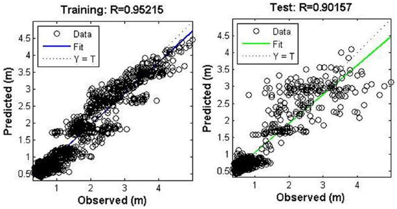
The scatter plot of training and simulation of the network during yearly predictions done using monthly data sets in the FFBP network.

Prediction using PSO-ANN

Weekly predictions

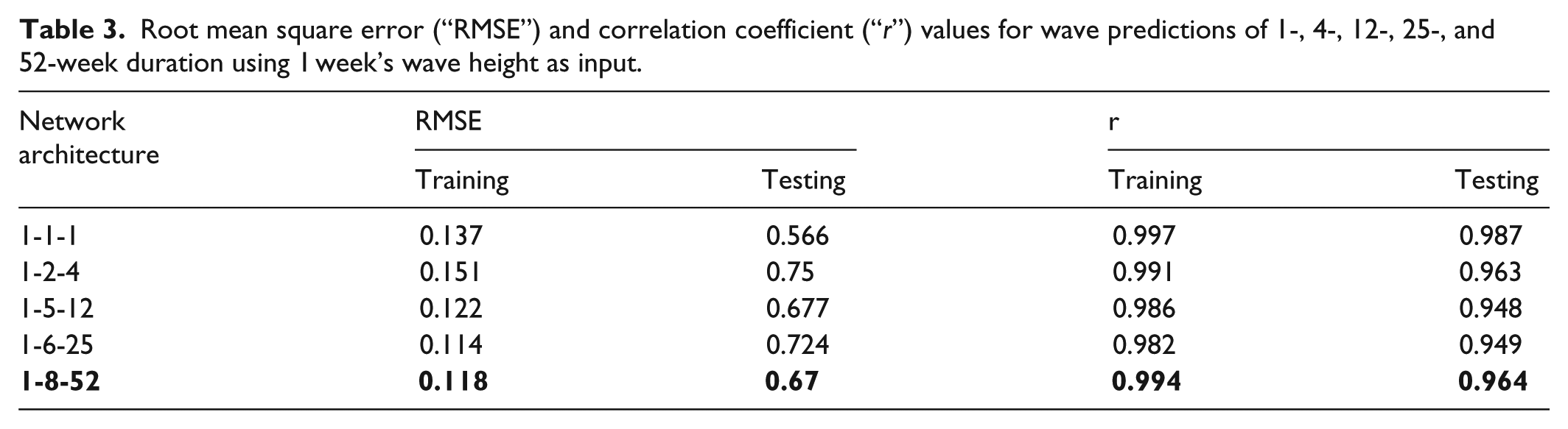
In this study, the PSO was applied to train the neural network for enhancing the convergence rate and the learning process. The learning process involves finding a set of weights that minimizes the learning error. Weekly predictions were carried out using 1 week’s input data to predict wave predictions of 4, 12, 25, and 52 weeks. The results obtained in terms of “MSE” and “r” were good, from 0.98 for 1 week’s prediction to greater than 0.96 for 52-week prediction. The variation of “r” values for the case is shown in Table 3. The increase in the number of neurons beyond eight led to a decrease in the prediction capability of the trained network. A scatter plot for training and simulation of the network for 52-week prediction is given in Figure 7. The “r” value will be 1 when the plot of observed versus predicted values follows a perfect straight line pattern passing through the origin. The time series plot of the observed versus predicted wave heights is shown in Figure 8.

Table 3.

Root mean square error (“RMSE”) and correlation coefficient (“r”) values for wave predictions of 1-, 4-, 12-, 25-, and 52-week duration using 1 week’s wave height as input.

Network architecture	RMSE		r
Network architecture	Training	Testing	Training	Testing
1-1-1	0.137	0.566	0.997	0.987
1-2-4	0.151	0.75	0.991	0.963
1-5-12	0.122	0.677	0.986	0.948
1-6-25	0.114	0.724	0.982	0.949
1-8-52	0.118	0.67	0.994	0.964

Figure 7.

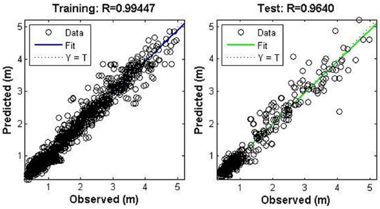
The scatter plot of training and simulation of the network during yearly predictions done using weekly data sets in the PSO-ANN network.

Figure 8.

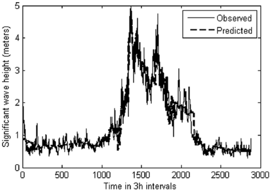
Graph showing the predicted and observed waves for the year 2006 using weekly data sets (1 January 2005 to 30 December 2005) in the PSO-ANN network.

Monthly predictions

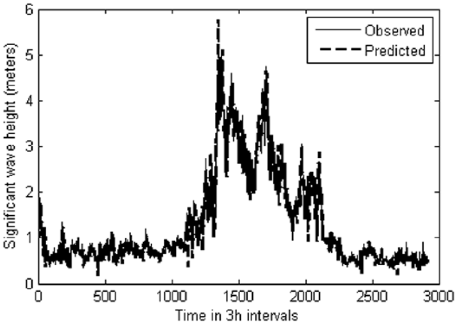
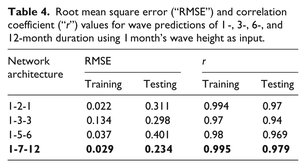
Monthly predictions were also carried out in similar way to that of weekly predictions using 1-month data set for predictions of waves with duration from 1 to 12 months, the results of which are tabulated in Table 4. One-year prediction can be obtained with accuracy greater than 0.97. The increase in neurons in the hidden layer beyond the best network architecture also showed gradual decrease in accuracy which would have rendered for 12-month prediction using 1-month data. Scatter plot and plot of observed versus predicted are shown in Figures 9 and 10.

Table 4.

Root mean square error (“RMSE”) and correlation coefficient (“r”) values for wave predictions of 1 -, 3-, 6-, and 12-month duration using 1 month’s wave height as input.

Network architecture	RMSE		r
Network architecture	Training	Testing	Training	Testing
1-2-1	0.022	0.311	0.994	0.97
1-3-3	0.134	0.298	0.97	0.94
1-5-6	0.037	0.401	0.98	0.969
1-7-12	0.029	0.234	0.995	0.979

Figure 9.

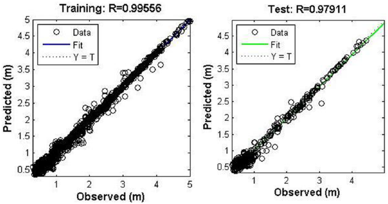
The scatter plot of training and simulation of the network during yearly predictions done using monthly data sets in the PSO-ANN network.

Figure 10.

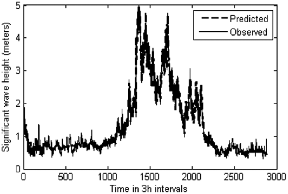
Graph showing the predicted and observed waves for the year 2006 using monthly data sets (1 January 2005 to 26 December 2005) in the PSO-ANN network.

Conclusions

ANN has been widely used in the field of coastal engineering for various applications. In this study, first the conventional FFBP network was used to predict the waves at New Mangalore Port Trust (NMPT) located along west coast of India, and the results were thereafter compared with those of the PSO-ANN model. The end results indicate that in the conventional FFBP network, the accuracy of the trained network depended on the length of the data segment used as input in model building, but in the case of the PSO-ANN network, accurate training was possible with relatively much smaller length of the input segment. In this application, the PSO-ANN network outperformed the conventional FFBP network in terms of the length of historical values used as input, training time, and accuracy.

Footnotes

Acknowledgements

The authors would like to thank New Mangalore Port Trust, Panambore, for providing us with the data of 8 months of continuous 3-hourly significant wave height measurements recorded at NMPT for this study.

Funding

The author(s) received no financial support for the research, authorship, and/or publication of this article.

Author biographies

Deepthi I Gopinath, hails from Kerala, India, completed her basic degree in Civil Engineering, and got her MTech [Marine Structures] from National Institute of Technology Karnataka, Surathakl in the year 2015. Her research area Applications of Artificial Neural Networks for Coastal and Ocean Engineering. She has 10+ publications in reputed journals and conferences.

GS Dwarakish, started his teaching career during 1993 and after completing his PhD in the area of Applications of RS & GIS for Coastal and Ocean Engineering, currently serving as Professor and Head of the Dept. of Applied Mechanics & Hydraulics, N.I.T.K., Surathkal, India. He has guided 14 BTech Projects, 31 MTech Dissertations, 7 MSc projects and 8 PhD scholars. Currently guiding 2 BTech Projects, 3 MTech Projects and 5 PhD scholars. He has completed 6 R & D projects and published 170 plus technical papers in International/National journals and conferences. He was a Guest Editor-In-Chief of special issue on Remote Sensing and GIS Applications of International Journal of Earth Sciences and Engineering and Editor of Aquatic Procedia, Vol.4, 2015, published by Elsevier.

References

Agrawal

Deo

(2004) Wave parameter estimation using neural network. Marine Structures 17: 536–550.

Altunkaynak

Ozger

(2004) Temporal significant wave height estimation from wind speed by perceptron Kalman filtering. Ocean Engineering 31: 1245–1255.

Asma

Sezer

Ozdemir

(2012) MLR and ANN models of significant wave height on the west coast of India. Computers & Geosciences 49: 231–237.

Balas

Koc

Balas

(2004) Predictions of missing wave data by recurrent neuronets. Journal of Waterway, Port, Coastal, and Ocean Engineering 130: 256–265.

Deo

(2010) Artificial neural networks in coastal and ocean engineering. Indian Journal of Geo-Marine Sciences 39: 589–596.

Deo

Jagdale

(2003) Prediction of breaking waves with neural networks. Ocean Engineering 30: 1163–1178.

Deo

Sridhar Naidu

(1999) Real time wave forecasting using neural network. Ocean Engineering 26: 191–203.

Deo

Jha

Chaphekar

(2001) Neural network for wave forecasting. Ocean Engineering 28: 889–898.

Dwarakish

Shetty

Usha

(2013) Review on applications of neural network in coastal engineering. CiiT International Journal of Artificial Intelligent Systems and Machine Learning 5: 324–331.

10.

Gunaydin

(2008) The estimation of monthly mean significant wave heights by using artificial neural network and regression methods. Ocean Engineering 35: 1406–1415.

11.

Jain

Deo

(2006) Neural network in ocean engineering. Ships and Offshore Structures 1: 25–35.

12.

Jain

Deo

(2007) Real-time wave forecasts off the western Indian coast. Applied Ocean Research 29: 72–79.

13.

Kalra

Deo

Kumar

(2005) RBF network for spatial mapping of wave heights. Marine Structures 18: 289–300.

14.

Kamranzad

Etemad-Shahidi

Kazeminezhad

(2011) Wave height forecasting in Dayyer, the Persian Gulf. Ocean Engineering 38: 248–255.

15.

Kennedy

Eberhart

(1995) Particle swarm optimization. In: Proceedings of the IEEE international joint conference on neural networks, Perth, WA, Australia, 27 November–1 December, pp. 1942–1948. New York: IEEE.

16.

Londhe

(2008) Soft computing approach for real-time estimation of missing wave heights. Ocean Engineering 35: 1080–1089.

17.

Londhe

Deo

(2003) Wave tranquility studies using neural networks. Marine Structures 16(6): 419–436.

18.

Londhe

Panchang

(2006) One-day wave forecasts based on artificial neural networks. Journal of Atmospheric and Oceanic Technology 23: 1593–1603.

19.

McCulloch

Pitts

(1943) A logical calculus of the ideas immanent in nervous activity. Bulletin of Mathematical Biophysics 5: 115–133.

20.

Mahjoobi

Etemad-Shahidi

(2008) An alternative approach for the prediction of significant wave heights based on classification and regression trees. Applied Ocean Research 30: 172–177.

21.

Mandal

Prabaharan

(2006) Ocean wave forecasting using recurrent neural networks. Ocean Engineering 33: 1401–1410.

22.

Mandal

Prabaharan

(2010) Ocean wave prediction using numerical and network models. The Open Ocean Engineering Journal 3: 12–17.

23.

Mandal

Patil

Manjunatha

. (2008) Applications of neural networks in coastal engineering—An overview. In: Proceedings of the 12th international conference of international association for computer methods and advances in geomechanics, pp. 1639–1645.

24.

Mandal

Rao

Raju

(2005) Ocean wave parameters estimation using backpropagation neural networks. Marine Structures 18: 301–318.

25.

Rakshith

Dwarakish

(2013) Review on applications on neural networks in coastal engineering. International Journal of Artificial Intelligence Systems and Machine Learning 5(7): 324–331.

26.

Rao

Mandal

(2005) Hindcasting of storm waves using neural network. Ocean Engineering 32: 667–684.

27.

Rao

Mandal

Prabaharan

(2001) Wave forecasting in near real time basis by neural network. In: Proceedings of the international conference in ocean engineering, 11–14 December, pp. 103–108. Ocean Engineering Centre, IIT Madras.

28.

Shiri

Makarynskyy

Kisi

. (2011) Prediction of short-term operational water levels using an Adaptive Neuro-Fuzzy Inference System. Journal of Waterway, Port, Coastal, and Ocean Engineering 137: 344–354.

29.

Tsai

Lin

Shen

(2002) Neural network for wave forecasting among multi-stations. Ocean Engineering 29: 1683–1695.

30.

Tsai

Lee

(1999) Back propagation neural network in tidal level forecasting. Journal of Waterway, Port, Coastal, and Ocean Engineering 125: 195–202.

31.

Zamani

Solomatine

Azimian

. (2008) Learning from data for wind–wave forecasting. Ocean Engineering 35: 953–962.

Real-time prediction of waves using neural networks trained by particle swarm optimization

Abstract

Keywords

Introduction

Study area and data products

Methodology

FFBP network

Particle swarm optimization–ANN network

Results and discussion

Prediction using FFBP network

Weekly predictions

Monthly predictions

Prediction using PSO-ANN

Weekly predictions

Monthly predictions

Conclusions

Footnotes

Acknowledgements

Funding

Author biographies

References