Fractional advection differential equation within Caputo and Caputo–Fabrizio derivatives

Abstract

In this research, we applied the variational homotopic perturbation method and q-homotopic analysis method to find a solution of the advection partial differential equation featuring time-fractional Caputo derivative and time-fractional Caputo–Fabrizio derivative. A detailed comparison of the obtained results was reported. All computations were done using Mathematica.

Introduction

In this research work, we have suggested the q-homotopic analysis method $(\mathrm{q}.\mathrm{HAM})$ and the variational homotopic perturbation method $(\mathrm{VHPIM})$ to find a solution for the advection partial differential equations $(\mathrm{PDEs})$ with time-fractional derivatives. We applied the methods based on Caputo–Fabrizio and Caputo derivatives^1,2 in order to compare the reported results. This work at first has been conducted in order to use the homotopic analysis method $(\mathrm{HAM})$ by Liao ³ and further to use it in order to solve PDEs featuring time-fractional derivative. El-Tawil and Huseen ⁴ proposed a method called $\mathrm{q}.\mathrm{HAM}$ which is considered a more general method of HAM. There exists a supportive parameter n and h in $\mathrm{q}.\mathrm{HAM}$ such that on concession that $n=1$ , the standard HAM can be obtained. Otherwise, we consider the VHPIM. ⁵ It should be noted that there are no accurate analytical solutions for most of the fractional differential equations. Consequently, for such equations we have to employ some direct and iterative methods. Researchers have used variant methods to solve fractional differential equations (FDEs) and fractional partial differential equations (FPDEs) in recent years. These methods include Abdomina’s decomposition method,^6,7 variational iteration method $(\mathrm{VIM})$ ,^8,9 HPM,^10–12 and HAM.^13–17

There are some books and papers related to applications of fractional calculus fitting real data for interested readers.^18–22

This work is arranged as follows: in section “Preliminaries,” the preliminaries are introduced. In section “Fundamental notion of the q.HAM,” the description of the $\mathrm{q}.\mathrm{HAM}$ is offered. The VHPIM in section “Fundamental of VHPIM” is explained. In section “Application and consequences,” the application of $\mathrm{q}.\mathrm{HAM}$ and VHPIM to the advection differential equation featuring time-fractional derivative is illustrated and makes a comparison of $\mathrm{q}.\mathrm{HAM}$ and VHPIM featuring Caputo–Fabrizio and Caputo derivative, respectively. Finally, in section “Conclusion,” some conclusions regarding the proposed method are drawn.

Preliminaries

In this section, we introduced briefly Caputo’s fractional derivative ¹ and Caputo–Fabrizio fractional derivative.^23–26

Definition 2.1

A function $u(t)$ belongs to $\mathbf{R}$ , $t>0$ , is assumed to be in $C_{\beta }(\beta \in \mathbf{R})$ , on the occasion that be $n\in \mathbf{R}(>\beta )$ , that $u(t)=t^n{u}_1(t)$ , which $u_1(t)\in C[0,\infty )$ , which is considered to be in $C_{\beta }^l$ iff $u^{(l)}\in C_{\beta }$ , $l\in \mathbf{N}$ .

Definition 2.2

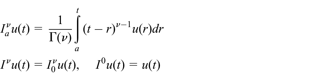
The fractional integral of $u(t)$ , $t>a$ , stated below is named Niemann-Knoxville fractional integral operator featuring $\nu >0$ , of a $u(t)\in C_{\beta }$ , $\beta \ge -1$ , will be stated in the form below

$$\begin{array}{c}{I}_a^{\nu }u(t)=\frac{1}{\Gamma (\nu )}\underset{a}{\overset{t}{\int }}{(t-r)}^{\nu -1}u(r)\mathrm{dr}\hfill \\ I^{\nu }u(t)=I_0^{\nu }u(t),I^{0}u(t)=u(t)\hfill \end{array}$$

Definition 2.3

The fractional derivative of $u(t)$ stated below is named Caputo’s fractional derivative

$$D^{\nu }u(t)=\frac{1}{\Gamma (l-\nu )}\underset{a}{\overset{t}{\int }}{(t-r)}^{l-\nu -1}{u}^{(l)}(r)\mathrm{dr}$$

for $u(t)\in C_{-1}^l$ , $l-1<\nu \le l$ , $t>a$ , and $l\in \mathbf{N}$ . ¹

Remark 2.4

The property below convinces ¹

$$I_a^{\nu }{D}_a^{\nu }u(t)=u(t)-\sum _{k=0}^{l-1}{u}^{(k)}(a^{+})\frac{{(t-a)}^k}{k!}$$

(1)

where $u\in C_{\beta }^l$ , $l\in \mathbf{N}$ , $\beta \ge -1$ , $l-1<\nu \le l$ , and $t>a$ .

Definition 2.5

The fractional derivative of $u(t)$ stated below is named Caputo–Fabrizio’s fractional derivative ²³

$${\mathcal{D}}_t^{\nu }u(t)=\frac{T(\nu )}{1-\nu }\underset{a}{\overset{t}{\int }}u\prime (r)\exp [-\frac{\nu (t-r)}{1-\nu }]\mathrm{dr}$$

(2)

in which $t>a$ , $0<\nu \le 1$ , and $T(\nu )$ is called the normalization function and it satisfies $T(0)=T(1)=1$ .

Definition 2.6

The fractional integral of $u(t)$ stated below is named Caputo–Fabrizio fractional integral

$${\mathcal{J}}_t^{\nu }u(t)=\frac{1-\nu }{T(\nu )}u(t)+\frac{\nu }{T(\nu )}\underset{a}{\overset{t}{\int }}u(r)\mathrm{dr},0<\nu \le 1$$

(3)

Remark 2.7

When $0<\nu \le 1$ , the property below convinces

$${\mathcal{J}}_a^{\nu }{\mathcal{D}}_a^{\nu }u(t)=u(t)-u(a)$$

(4)

Fundamental notion of the q.HAM

To explain the essential notions of the $\mathrm{q}.\mathrm{HAM}$ for time-fractional PDEs, we consider

$$\mathcal{N}(u(x,t))=f(x,t)$$

(5)

in which $u(x,t)$ is an unfamiliar function, $\mathcal{N}$ is an operator nonlinear and linear, t and x denote the independent variables, and $D^{\nu }$ denotes that Caputo fractional derivative or Caputo–Fabrizio fractional derivative featuring $0<\nu \le 1$ . First, we construct the zero-order modified equation as

$$\begin{array}{c}(1-nq)\mathcal{L}[\psi (x,t;q)-u_0(x,t)]=qhW(x,t)\times \hfill \\ (\mathcal{N}[\psi (x,t;q)]-f(x,t))\hfill \end{array}$$

(6)

here $n>1$ , $q\in [0,1/n]$ is the embedded parameter, $h\ne 0$ is a supportive parameter, $W(x,t)\ne 0$ is a supportive function, $\mathcal{L}$ is a supportive linear operator, and $u_0(x,t)$ is primary speculation. Clearly, since $q=0$ and $q=1/n$ , equation (6) turns out to be

$$\psi (x,t;0)=u_0(x,t),\psi (x,t;\frac{1}{n})=u(x,t)$$

(7)

in the state order. Therefore, q goes up from $0$ to $1/n$ , the answer $\psi (x,t;q)$ changes to the primary speculation $u_0(x,t)$ to $u(x,t)$ . If $u_0(x,t)$ , $\mathcal{L}$ , h, and $W(x,t)$ are selected suitably, answer of equation (7) exists for $q\in [0,1/n]$ .

Here, we consider the Taylor series expression of $\psi (x,t;q)$ with respect to q in

$$\varphi (x,t;q)=\sum _{m=0}^{\infty }{u}_m(x,t)q^m$$

(8)

where

$${\varphi }_m(x,t)=\frac{1}{m!}\frac{d^m}{d{q}^m}{\phi }_m(x,t;q){|}_{q=0}$$

(9)

It is supposed that the supportive linear operator, the primary speculation, the supportive parameter h, and the supportive function $W(x,t)$ are opted so, equation (8) is convergent when $q\to 1/n$ . Following that the rough answer (8) can be represented as

$$u(x,t)=\varphi (x,t;\frac{1}{n})=\sum _{m=0}^{\infty }{u}_m(x,t){\left(\frac{1}{n}\right)}^m$$

(10)

Then, we can express the vector

$${\overrightarrow{u}}_n(x,t)=\{u_0(x,t),u_1(x,t),u_2(x,t),\dots ,u_n(x,t)\}$$

(11)

After mth-order derivation of equation (6) by attention to q, next with $q=0$ , the mth-order modified equation is given as

$$\mathcal{L}[u_m(x,t)-{\chi }_m{u}_{m-1}u(x,t)]=\mathrm{hW}(x,t){\mathcal{R}}_m({\overrightarrow{u}}_{m-1}(x,t))$$

(12)

with primary concessions

$$u_m^{(n)}(x,t)=0,n=0,1,2,3,\dots ,m-1$$

(13)

where

$$\begin{array}{c}{\mathcal{R}}_m({\overrightarrow{u}}_{m-1}(x,t))=-(f(x,t)-\frac{{\chi }_m}{n}f(x,t))\hfill \\ +\frac{1}{(m-1)!}\frac{d^{m-1}}{d{q}^{m-1}}\mathcal{N}(x,t;q){|}_{q=0}\hfill \end{array}$$

(14)

and

$${\chi }_m=\{\begin{array}{c}n,m>1\hfill \\ \multicolumn{1}{c}{0,m\le 1}\end{array}$$

(15)

Operating the Niemann-Knoxville integral operator $I^{\nu }$ on both sides of equation (12)

$$\begin{array}{c}{u}_m(x,t)={\chi }_m{u}_{m-1}(x,t)-{\chi }_m(u_{m-1}(x{,0}^{+}))\hfill \\ +hW(x,t)I^{\nu }{\mathcal{R}}_m({\overrightarrow{u}}_{m-1}(x,t))\hfill \end{array}$$

(16)

With regard to the fact that $u_m(x,t),m\ge 1$ is controlled by equation (12) featuring linear boundary concessions that are resultant from the initial problem.

As a result of the existence of the factor $(1/n{)}^m$ , there will be more chance for the occurrence of convergence or even we can achieve faster convergence in comparison with the standard HAM.

Fundamental of VHPIM

In this part, we assume VHPIM in two stages for equation (5), featuring

$$\mathcal{N}(u(x,t))=D_t^{\nu }u(x,t)-\mathcal{K}u(x,t)$$

(17)

in which $0<\nu \le 1$ and $\mathcal{K}$ in which derivatives concerning t and x, is an operator in t, and x. Now, VHPIM is introduced in the following two stages.

Stage 1

Conforming to VIM, we construct the rectification functional for formula (5)

$$\begin{array}{c}{u}_{j+1}(x,t)=u_j(x,t)+I^{\nu }[\theta (t)(D^{\nu }{u}_j(x,t)-\hfill \\ \mathcal{K}({\stackrel{⌣}{u}}_j,({\stackrel{⌣}{u}}_j{)}_x,({\stackrel{⌣}{u}}_j{)}_{\mathrm{xx}})-f(x,t))]\hfill \\ =u_j(x,t)\hfill \\ +\frac{1}{\Gamma (\nu )}\underset{0}{\overset{t}{\int }}{(t-r)}^{\nu -1}\theta (r)(D^{\nu }{u}_j(x,r)\hfill \\ -\mathcal{K}({\stackrel{⌣}{u}}_j,({\stackrel{⌣}{u}}_j{)}_x,({\stackrel{⌣}{u}}_j{)}_{\mathrm{xx}})-f(x,r))\mathrm{dr}\hfill \end{array}$$

(18)

Here, $I^{\nu }$ implies the Niemann-Knoxville fractional integral, and $\theta$ is a Lagrange coefficient, that can be recognized as optimal by variational approach. The function ${\stackrel{⌣}{u}}_k$ is supposed as a limited variation. In other words, $\delta {\stackrel{⌣}{u}}_k=0$ .

Stage 2

By utilizing the HPM and VIM, we obtain the below formula

$$\begin{array}{c}\sum _{j=0}^{\infty }{p}^n{u}_j(x,t)=u_0(x,t)+p\{\sum _{j=1}^{\infty }{p}^j{u}_j(x,t)+\hfill \\ I^{\nu }(\theta (t)(\sum _{j=0}^{\infty }{p}^j{D}^{\nu }{u}_j(x,t)-\hfill \\ \sum _{j=0}^{\infty }{p}^j\mathcal{K}({\stackrel{⌣}{u}}_j,({\stackrel{⌣}{u}}_j{)}_x,({\stackrel{⌣}{u}}_j{)}_{\mathrm{xx}})-\hfill \\ f(x,t)))\}\hfill \end{array}$$

(19)

In equation (19), $p\in [0,1]$ is a secured parameter and $u_0$ is a primary estimate of formula (5).

Balancing the sentences featuring the same powers of p in two sides of the formula (18), we may obtain $u_j(j=0,1,2,\dots )$ .

Eventually, conforming to HPM, when p tends to be $1$ , we can gain the answer with approximation

$$u(x,t)=\sum _{j=0}^{\infty }{u}_j(x,t)$$

(20)

Differently, conforming to VIM, the rectification functional (19) that may be uttered by approximation is stated as

$$\begin{array}{c}{u}_{j+1}(x,t)=u_j(x,t)+\underset{0}{\overset{t}{\int }}\theta (r)(\frac{d}{\mathrm{dt}}u(x,r)-\hfill \\ \mathcal{K}({\stackrel{⌣}{u}}_j,({\stackrel{⌣}{u}}_n{)}_x,({\stackrel{⌣}{u}}_j{)}_{\mathrm{xx}})-f(x,r))\mathrm{dr}\hfill \end{array}$$

(21)

where ${\stackrel{⌣}{u}}_j$ is a rectification functional; however, ${\stackrel{⌣}{u}}_j$ is assumed as a surrounded variation, that is, $\delta {\stackrel{⌣}{u}}_j(x,t)=0$ .

Afterward, by creating functional stationary

$$\begin{array}{c}\delta u_{j+1}(x,t)=\delta u_j(x,t)+\hfill \\ \delta \underset{0}{\overset{t}{\int }}\theta (r)(\frac{d^m}{d{t}^m}u(x,r)-f(x,r))\mathrm{dr}\hfill \end{array}$$

the Lagrange multiplier will be equal to $\theta =-1$ . Thus, the following repetition rule to be earned

$$\begin{array}{c}{u}_{j+1}(x,t)=u_j(x,t)-\hfill \\ I^{\nu }(D^{\nu }{u}_j(x,t)-\mathcal{K}{u}_j(x,t)-f(x,t))\hfill \end{array}$$

(22)

Applying equation (19), we can create the repetition rule as follows

$$\begin{array}{c}\sum _{j=0}^{\infty }{p}^j{u}_j(x,t)=u_0(x,t)+p\{\sum _{j=1}^{\infty }{p}^j{u}_j(x,t)+\hfill \\ I^{\nu }(\sum _{j=0}^{\infty }{p}^j{D}^{\nu }{u}_j(x,t)-\sum _{j=0}^{\infty }{p}^j\mathcal{K}({\stackrel{⌣}{u}}_j,({\stackrel{⌣}{u}}_j{)}_x,({\stackrel{⌣}{u}}_j{)}_{\mathrm{xx}})\hfill \\ -f(x,t))\}\hfill \end{array}$$

(23)

Balanced with the coefficient of some power of p in two hands of equation (23), we can get $u_i(x,t),(i=0,1,2,\dots )$ . As a consequence HPM, we can gain an answer of equation (5)

$$u(x,t)=\sum _{j=0}^{\infty }{u}_j(x,t)$$

Application and consequences

In this portion, we utilize $\mathrm{q}.\mathrm{HAM}$ and VHPIM to solve time-fractional advection PDE

$$D_t^{\nu }u(x,t)+u_x(x,t)u(x,t)=x(1+t^2)$$

(24)

where $0<\nu \le 1$ , $t>0$ , and $x\in \mathbb{R}$ is chosen featuring the primary status

$$u(x,0)=0$$

(25)

With the replacement of the primary status $u(x,0)$ in the recurrent formula (16), the consequence with $\mathrm{q}.\mathrm{HAM}$ featuring Caputo derivative is stated as

$$\begin{array}{l}{u}_0(x\mathrm{,}t)=0\\ u_1(x\mathrm{,}t)=-\frac{hx{t}^{\nu }\left({\nu }^2+3\nu +2+2t^2\right)}{\Gamma (\nu +3)}\end{array}$$

$$\begin{array}{l}{u}_2(x\mathrm{,}t)=-\frac{hnx{t}^{\nu }\left({\nu }^2+3\nu +2+t^2\right)}{\Gamma (\nu +3)}+\\ \frac{h^4{t}^{3\nu }{x}^2\nu +2(-16t^{4}2\nu +3(2(\nu +3)(2\nu +5)t^2}{3\Gamma {(\nu +3)}^2\Gamma (3\nu +3)\Gamma (3\nu +7)}+\\ \frac{3(\nu +2)(3\nu +5)({\nu }^2+3\nu +3)\Gamma (2\nu +2)\Gamma (3\nu +4)}{3\Gamma {(\nu +3)}^2\Gamma (3\nu +3)\Gamma (3\nu +7)}-\\ \frac{3(\nu +{1)}^2\Gamma (2\nu +1)\Gamma (3\nu +7)\left(9{\nu }^2(\nu +3)+20\nu \right))}{3\Gamma {(\nu +3)}^2\Gamma (3\nu +3)\Gamma (3\nu +7)}+\\ \frac{2(2\nu +1)(\nu (\nu +3)+6)t^2+4}{3\Gamma {(\nu +3)}^2\Gamma (3\nu +3)\Gamma (3\nu +7)}\\ \cdots \end{array}$$

Then, we consider the first three sentences with $n=1$ as estimates of answer for formula (24)

$$\begin{array}{c}u(x,t)\approx -\frac{\mathrm{hx}{t}^{\nu }({\nu }^2+3\nu +2+2t^2)}{\Gamma (\nu +3)}-\hfill \\ \frac{\mathrm{hnx}{t}^{\nu }({\nu }^2+3\nu +2+2t^2)}{\Gamma (\nu +3)}+\hfill \\ \frac{h^4{t}^{3\nu }{x}^2\nu +2(-16t^{4}2\nu +3(2(\nu +3)(2\nu +5)t^2}{3\Gamma {(\nu +3)}^2\Gamma (3\nu +3)\Gamma (3\nu +7)}+\hfill \\ \frac{3(\nu +2)(3\nu +5)(\nu (\nu +3)+3))\Gamma (2\nu +2)\Gamma (3\nu +4)}{3\Gamma {(\nu +3)}^2\Gamma (3\nu +3)\Gamma (3\nu +7)}-\hfill \\ \frac{3(\nu +{1)}^2\Gamma (2\nu +1)\Gamma (3\nu +7)(9{\nu }^2(\nu +3)+20\nu ))}{3\Gamma {(\nu +3)}^2\Gamma (3\nu +3)\Gamma (3\nu +7)}+\hfill \\ \frac{2(2\nu +1)(\nu (\nu +3)+6)t^2+4}{3\Gamma {(\nu +3)}^2\Gamma (3\nu +3)\Gamma (3\nu +7)}\hfill \end{array}$$

(26)

Now, when the incipient value $u(x,0)$ is substituted into the recursive equation (16), with $\mathrm{q}.\mathrm{HAM}$ featuring Caputo–Fabrizio derivative, we can obtain

$$\begin{array}{c}{u}_0(x,t)=0\hfill \\ u_1(x,t)=-\frac{1}{3}\mathrm{hx}(-3\nu +t(\nu (t^2-3t+3)+3t)+3)\hfill \\ u_2(x,t)=\frac{1}{315}\mathrm{hx}(-105\mathrm{ht}(\nu (t^2-3t+3)+3t)-\hfill \\ h^2(-315(\nu -{1)}^3+\nu (\nu (15\nu -26)+13)t^5+\hfill \\ 945(\nu -1{)}^2\nu t-70(\nu -1){\nu }^2{t}^6+5{\nu }^3{t}^7-\hfill \\ 630(\nu -1)(2(\nu -1)\nu +1)t^2-\hfill \\ 21105\nu (\nu (11\nu -20)+10)t^3))+\hfill \\ 105(\nu -1)(\nu (7\nu -6)+3)t^4+\hfill \\ 105\mathrm{nt}(\nu ((t-3)t+3)+3t)\hfill \\ \cdots \hfill \end{array}$$

The first three statements for approximate answer for equation (24) will be stated as

$$\begin{array}{c}u(x,t)\approx -\frac{1}{3}\mathrm{hx}(-3\nu +t(\nu (t^2-3t+3)+3t)+3)+\hfill \\ \frac{1}{315}\mathrm{hx}(-105\mathrm{ht}(\nu (t^2-3t+3)+3t)-\hfill \\ 105\mathrm{nt}(\nu ((t-3)t+3)+3t)+\hfill \\ h^2(-315(\nu -{1)}^3+945(\nu -{1)}^2\nu t-\hfill \\ 70(\nu -1){\nu }^2{t}^6+5{\nu }^3{t}^7-\hfill \\ 630(\nu -1)(2(\nu -1)\nu +1)t^2-\hfill \\ 105(\nu -1)(\nu (7\nu -6)+3)t^4+\hfill \\ 105\nu (\nu (11\nu -20)+10)t^3+\hfill \\ 21\nu (\nu (15\nu -26)+13)t^5))\hfill \end{array}$$

(27)

Substituting the incipient value $u(x,0)$ within the recurrent formula (16), the consequence with VHPIM featuring Caputo derivative will be

$$\begin{array}{c}{u}_0(x,t)=0\hfill \\ u_1(x,t)=\frac{x{t}^{\nu }({\nu }^2+3\nu +2t^2+2)}{\nu ({\nu }^2+3\nu +2)\Gamma (\nu )}\hfill \\ u_2(x,t)=\frac{x{t}^{\nu }({\nu }^2+3\nu +2t^2+2)}{\nu ({\nu }^2+3\nu +2)\Gamma (\nu )}-\hfill \\ \frac{t^{\nu }x}{\Gamma {(\nu )}^2}(\frac{\pi \csc (\pi \nu )\Gamma (\nu )(\Gamma (\nu +3)+2t^2\Gamma (\nu +1))}{\Gamma (1-\nu )\Gamma (\nu +1)\Gamma (\nu +3)}+\hfill \\ (t^{2\nu }(4t^4\Gamma (2\nu +5)\Gamma (3\nu +1)\Gamma (3\nu +3)+\hfill \\ {\nu }^2+3\nu +2(4t^2\Gamma (2\nu +3)\Gamma (3\nu +1)+\hfill \\ ({\nu }^2+3\nu +2)\Gamma (2\nu +1)\Gamma (3\nu +3))\Gamma (3\nu +5)))/\hfill \\ {\nu }^2{({\nu }^2+3\nu )}^2\Gamma (3\nu +1)\Gamma (3\nu +3)\Gamma (3\nu +5))\hfill \\ \cdots \hfill \end{array}$$

Then, consider the first three sentences with $n=1$ as estimates of answer for formula (24) are

$$\begin{array}{c}u(x,t)\approx \frac{x{t}^{\nu }({\nu }^2+3\nu +2t^2+2)}{\nu ({\nu }^2+3\nu +2)\Gamma (\nu )}+\hfill \\ \frac{x{t}^{\nu }({\nu }^2+3\nu +2t^2+2)}{\nu ({\nu }^2+3\nu +2)\Gamma (\nu )}-\hfill \\ \frac{t^{\nu }x}{\Gamma {(\nu )}^2}(\frac{\pi \csc (\pi \nu )\Gamma (\nu )(\Gamma (\nu +3)+2t^2\Gamma (\nu +1))}{\Gamma (1-\nu )\Gamma (\nu +1)\Gamma (\nu +3)}+\hfill \\ (t^{2\nu }(4t^4\Gamma (2\nu +5)\Gamma (3\nu +1)\Gamma (3\nu +3)+\hfill \\ {\nu }^2+3\nu +2(4t^2\Gamma (2\nu +3)\Gamma (3\nu +1)+\hfill \\ ({\nu }^2+3\nu +2)\Gamma (2\nu +1)\Gamma (3\nu +3))\Gamma (3\nu +5)))/\hfill \\ {\nu }^2{({\nu }^2+3\nu +2)}^2\Gamma (3\nu +1)\Gamma (3\nu +3)\Gamma (3\nu +5))\hfill \end{array}$$

Now, when the initial amount $u(x,0)$ is substituted into the iteration (16), with VHPIM featuring Caputo–Fabrizio derivative

$$\begin{array}{c}{u}_0(x,t)=0\hfill \\ u_1(x,t)=\frac{1}{3}\nu t^{3}x-\nu t^{2}x+t^{2}x+\nu \mathrm{tx}-\nu x+x\hfill \\ u_2(x,t)=(\nu -2)(\nu -1)\nu x-3(\nu -1{)}^2\nu \mathrm{tx}+\hfill \\ \frac{2}{9}(\nu -1){\nu }^2{t}^{6}x-\frac{1}{3}(\nu -1)(\nu (7\nu -6)+3)t^{4}x\hfill \\ \frac{1}{63}{\nu }^3{t}^{7}x+2(\nu -1)(2(\nu -1)\nu +1)t^{2}x-\hfill \\ \frac{1}{3}\nu (\nu (11\nu -20)+10)t^{3}x-\hfill \\ \frac{1}{15}\nu (\nu (15\nu -26)+13)t^{5}x\hfill \\ \cdots \hfill \end{array}$$

Following that, the third sequence term approximate answer for formula (24) is stated as

$$\begin{array}{c}u(x,t)\approx \frac{1}{3}\nu t^{3}x-\nu t^{2}x+t^{2}x+\nu \mathrm{tx}-\nu x+x+\hfill \\ (\nu -2)(\nu -1)\nu x-3(\nu -1{)}^2\nu \mathrm{tx}+\hfill \\ \frac{2}{9}(\nu -1){\nu }^2{t}^{6}x-\frac{1}{3}(\nu -1)(\nu (7\nu -6)+3)t^{4}x+\hfill \\ \frac{1}{63}{\nu }^3{t}^{7}x+2(\nu -1)(2(\nu -1)\nu +1)t^{2}x-\hfill \\ \frac{1}{3}\nu (\nu (11\nu -20)+10)t^{3}x-\hfill \\ \frac{1}{15}\nu (\nu (15\nu -26)+13)t^{5}x\hfill \end{array}$$

(28)

In Tables 1 and 2, we may observe the rough answers for $\nu =1.0$ , that is taken for several values of x and t using $\mathrm{q}.\mathrm{HAM}$ and VHPIM with two fractional derivatives, involving singular differential operator which is named Caputo and involving nonsingular differential operator which is named Caputo–Fabrizio.

Table 1.

Estimate values with VHPIM when $\nu =1$ for equation (24).

Approximate answer
t	x	$u_{\mathrm{Exact}}$	Caputo	Caputo–Fabrizio
0.3	0.50	0.15	0.149836	0.149836
	0.75	0.225	0.224754	0.224754
	1.00	0.30	0.299673	0.299673
0.5	0.50	0.25	0.247855	0.247855
	0.75	0.375	0.371782	0.371782
	1.00	0.50	0.495709	0.495709
0.7	0.50	0.35	0.338142	0.338142
	0.75	0.525	0.507213	0.507213
	1.00	0.70	0.676283	0.676283

Table 2.

Estimate values with $\mathrm{q}.\mathrm{HAM}$ when $\nu =1$ , $h=-1$ , and $n=1$ for equation (24).

Approximate answer
t	x	$u_{\mathrm{Exact}}$	Caputo	Caputo–Fabrizio
0.3	0.50	0.15	0.150334	0.150334
	0.75	0.225	0.225500	0.225500
	1.00	0.30	0.299673	0.299673
0.5	0.50	0.25	0.248333	0.248333
	0.75	0.375	0.372499	0.372499
	1.00	0.50	0.496666	0.496666
0.7	0.50	0.35	0.348534	0.348534
	0.75	0.525	0.507832	0.507832
	1.00	0.70	0.677110	0.677110

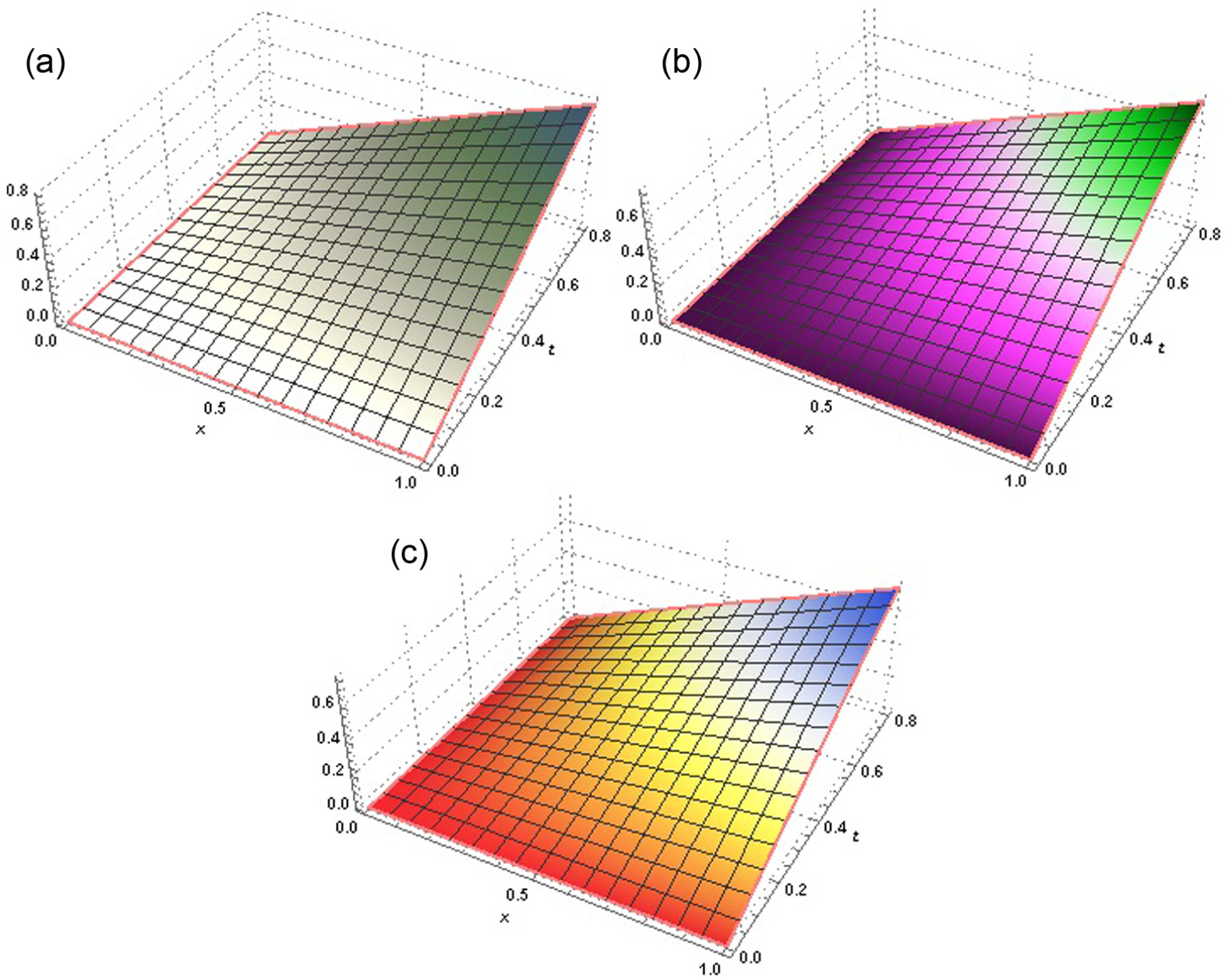
We can see the accrue and estimate answers with $\mathrm{q}.\mathrm{HAM}$ toward $\nu =1$ , in Figure 1 with VHPIM.

Figure 1.

(a) The estimate answer, (b) approximate answer featuring Caputo-Fabrizio derivative with VHPIM, and (c) approximate answer featuring Caputo derivative with VHPIM.

In Figure 2, we can see the accrue and estimate answers toward $h=-1$ , $n=1$ , and $\nu =1$ with $\mathrm{q}.\mathrm{HAM}$ .

Figure 2.

(a) The estimate answer, (b) approximate answer featuring Caputo-Fabrizio derivative with q.HAM, and (c) approximate answer featuring Caputo derivative with q.HAM.

In Table 3, the list of the times in seconds for every iteration in two methods used by CPU has been shown.

Table 3.

List of the times in seconds used.

	VHPIM		$\mathrm{q}.\mathrm{HAM}$
	Caputo	Caputo–Fabrizio	Caputo	Caputo–Fabrizio
$u_0(x,t)$	0	0	0	0
$u_1(x,t)$	2.359375	0.015625	2.359375	0.015625
$u_2(x,t)$	16.312500	3.968750	18.625000	4.328125

Conclusion

In this work, we have prosperously applied $\mathrm{q}.\mathrm{HAM}$ and VHPIM to compare between Caputo and Caputo–Fabrizio derivatives for the time-fractional advection partial differential equation. The results indicate that rough answers for both derivatives for both methods are similar. And the Caputo–Fabrizio derivative is faster than the Caputo derivative in terms of CPU speed in calculation in Mathematica.