
Abstract
The aim of this article is to analyze the dynamics of the new chaotic system in the sense of two fractional operators, that is, the Caputo–Fabrizio and the Atangana–Baleanu derivatives. Initially, we consider a new chaotic model and present some of the fundamental properties of the model. Then, we apply the Caputo–Fabrizio derivative and implement a numerical procedure to obtain their graphical results. Further, we consider the same model, apply the Atangana–Baleanu operator, and present their analysis. The Atangana–Baleanu model is used further to present a numerical approach for their solutions. We obtain and discuss the graphical results to each operator in details. Furthermore, we give a comparison of both the operators applied on the new chaotic model in the form of various graphical results by considering many values of the fractional-order parameter
Introduction
Chaotic models are widely considered due to their applications in many branches of engineering and science and, especially, a rapid increase in the form of publications on chaotic models has been observed.1–7 Particularly, chaotic models are considered for practical purposes in many areas, such as chaotic communication, 2 image watermarking, 1 and autonomous mobile robots. 3 Due to the applications of chaotic models, the researchers developed some new chaotic models and presented their analysis.4,5 The literature shows clearly that most of the chaotic models have unstable equilibrium points,6,7 and such system exhibits self-excited attractors. 7 Some other chaotic models that are studied by the researchers in order to identify their chaotic dynamics can be seen in Wei et al.8–10 and the references therein.
The fractional-order modeling has gained a lot of attentions from the researchers once the new operators are defined. In these newly defined operators, the operator Caputo–Fabrizio and the Atangana–Baleanu derivative received more attention from the researchers, and various articles have been proposed on these, including the Caputo derivative.11–18 There are many applications of the fractional models, such as the generalization of the model and the memory effects, which are usually attached to the real-life problems. The fractional-order modeling has the advantage of observing the dynamics of the real-life problems at any point of interests where such analysis for the integer-order models does not exist. The crossover behavior of the non-linear problems can only be handled by the newly introduced derivatives.
The chaotic systems studied in fractional calculus are numerous in literature.19–24 A fractional chaotic model and its application to chaotic system have been discussed in the work of Atangana. 24 A fractional model with no-indexed law and its application to chaos and statistics have been considered in the work of Atangana and Gómez-Aguilar. 23 Owolabi and Atangana 22 considered a chaotic model in integer case and presented its dynamical analysis. Zhang et al. 21 considered a delayed chaotic model and analyzed its dynamics. A fractional chaotic model with no equilibrium has been discussed in the work of Mishra. 20 Su et al. 19 presented a chaotic model and obtained a numerical scheme. Recently, a fractional logistic map and its application to dynamical analysis have been studied by Yuan et al. 25 The real data application of fractional calculus to blood ethanol concentration calculation has been considered in Qureshi et al. 26 The dynamics of chickenpox disease with field data is studied through fractional derivative in Qureshi and Yusuf. 27 Application of the new derivatives to the partial differential equations is considered in Yusuf et al. 28 A two-strain epidemic model with fractional derivatives has been proposed in Yusuf et al. 29 The application of fractional operator known as Atangana–Baleanu to Korteweg–de Vries (KDV) equation is analyzed in Inc et al. 30 The dynamics of chaotic attractors with fractional conformable derivative is proposed in Pérez et al. 31 A fractional-time wave equation with regular kernel is studied by Cuahutenango-Barro et al. 32 The authors studied a fractional Hunter–Saxton equation using Riemann–Liouville and Liouville–Caputo derivatives. 33 Numerical solution of Fisher’s type equations of fractional nature with Atangana–Baleanu derivative is considered in Saad et al. 34 The application of Feng’s first integral technique to the fractional modified Korteweg–de Vries (MKDV) equation and their analysis and solutions is presented in Yépez-Martnez et al. 35
Motivated from the recent literature on the chaotic models, we consider a new chaotic model in two fractional operators, that is, the Caputo–Fabrizio derivative and the Atangana–Baleanu derivative, and present comparison results. Then, we present numerical approaches for both the derivatives and give various graphical results for the fractional-order parameter
Basic concepts of Caputo–Fabrizio and Atangana–Baleanu derivative
This section presents the basic concepts regarding the two fractional operators, namely, Caputo–Fabrizio and Atangana–Baleanu derivatives as follows:
Definition 1
Let

where the normal function is given by
Remark 1
If

Moreover

The following integral associated with the derivative above is defined as follows 37
Definition 2
Let

Remark 2
In definition 2, the remainder of the integral of the function with

gives
Losada and Nieto 37 used the result given by equation (6) and presented the following definition

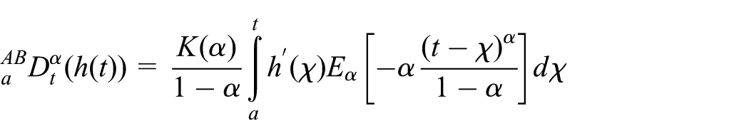
Next, we recall the fundamental concept of Atangana–Baleanu derivative 38 and the related results.
Definition 3
Let
Definition 4
Let

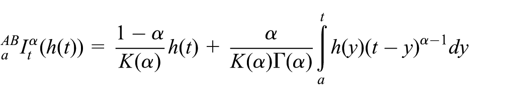
Definition 5
The fractional integral with non-local kernel of Atangana–Baleanu fractional derivative is given by
Further, we present the following results.
Theorem 1
On

Theorem 2
Atangana–Baleanu and Atangana–Baleanu-R derivatives fulfill the Lipschitz conditions and are shown by 38

and

Theorem 3
For the given fractional differential equation 38

by applying the inverse Laplace transform and the convolution, we have a unique solution 38
Model framework
Here, we consider a new chaotic model considered in Wang et al. 39 and is given by

where the state variables are shown by
The fractional Caputo–Fabrizio derivative form of the system equation (13) will be

To find the equilibrium point of the model equation (14), we put the right-hand side of the model equation (14) equal to zero and obtain

The Jacobian matrix at the equilibrium point P of the model (14) is

The characteristic equation for the Jacobian matrix
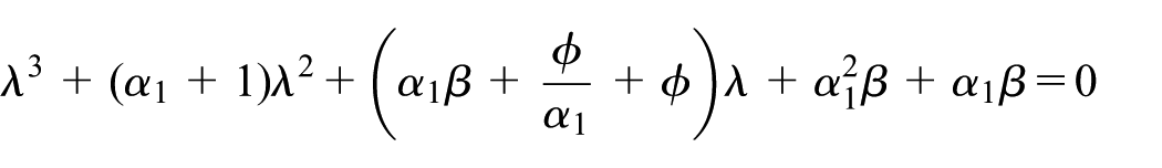
and the Routh–Hurwitz criteria can be easily satisfied

This shows that the fractional system (14) has one stable equilibrium point. Further, the system (14) is dissipative and can be easily obtained by taking the partial derivative of each variable of the model (14), and on adding, we get
Numerical approach for Caputo–Fabrizio derivative
The model given in Caputo–Fabrizio form (14) is used to obtain a numerical scheme by considering the scheme presented in Atangana and Owolabi.
40
The obtained scheme is used further to obtain the graphical results for the model in Caputo–Fabrizio–order derivative (14) by taking different values of

For

Further, we obtain the following equation

We approximate the function

where
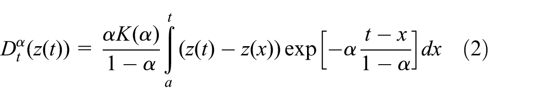
The approximations described above is used and we obtain the integral in equation (2)
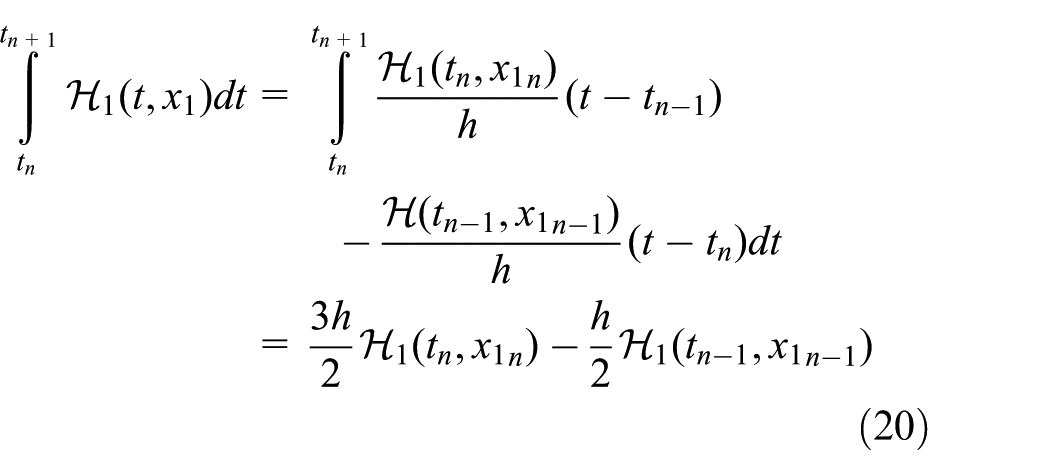
Using equation (20) in equation (2), after some calculations, we have

Using the procedure presented above in the same manner for the rest of the equations of the Caputo–Fabrizio model (14), we have

Using the procedure presented above for the solution of the Caputo–Fabrizio model (14), we obtain the graphical results in Figures 1–8 by taking

Considering the model (14) when
Considering the model (14) when

Considering the model (14) when
Considering the model (14) when

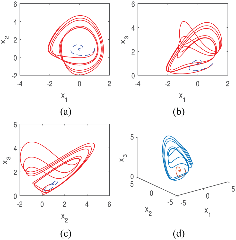
Considering the model (14) when α = 1, shows chaotic attractor: (a) Phase portraits (x1-x2 plane), (b) Phase portraits (x1-x3 plane), (c) Phase portraits (x2-x3 plane) and (d) 3D plot (x1-x2-x3 plane).

Considering the model (14) when α = 0.95, shows chaotic attractor: (a) Phase portraits (x1-x2 plane), (b) Phase portraits (x1-x3 plane), (c) Phase portraits (x2-x3 plane) and (d) 3D plot (x1-x2-x3 plane).

Considering the model (14) when α = 0.9, shows chaotic attractor: (a) Phase portraits (x1-x2 plane), (b) Phase portraits (x1-x3 plane), (c) Phase portraits (x2-x3 plane) and (d) 3D plot (x1-x2-x3 plane).
Considering the model (14) when
Model in Atangana–Baleanu derivative form
The model given by equation (13) can be written in fractional Atangana–Baleanu derivative form as

Numerical procedure for Atangana–Baleanu derivative
Here, we give a procedure, similar to Khan et al. 14 , for the numerical solution of the model in the form of Atangana–Baleanu derivative equation (23) by considering the method explained in Toufik and Atangana, 41 which is effectively used for many problems that belong to the real-world life. We consider the same approach presented in Toufik and Atangana 41 and apply it on our model (23) as per the following: before we proceed to start the approach, first, we write the model in Atangana–Baleanu shape (equation (23)) in the form given below

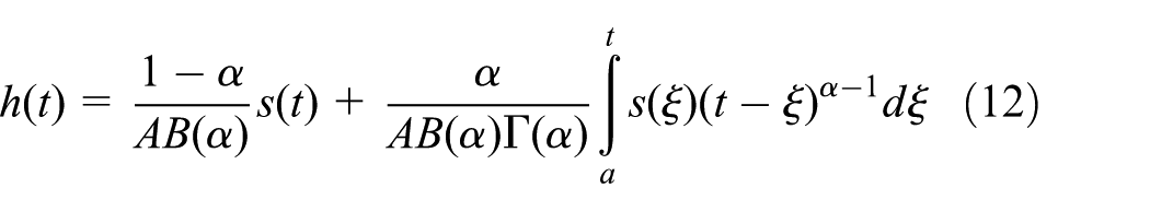
The model given by equation (23) can be expressed in the form after using the fundamental theorem of integration
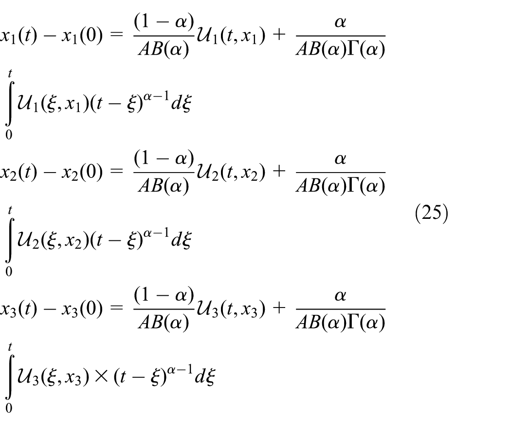
We get from equation (25) for


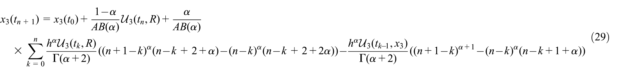
Using the integral given in equation (26), approximated using the two-point interpolation polynomial, we have the following iterative scheme for the model (23) after some simplifications. Using the same procedure for the remaining equations of Atangana–Baleanu model (23), we have the recursive formula as given by

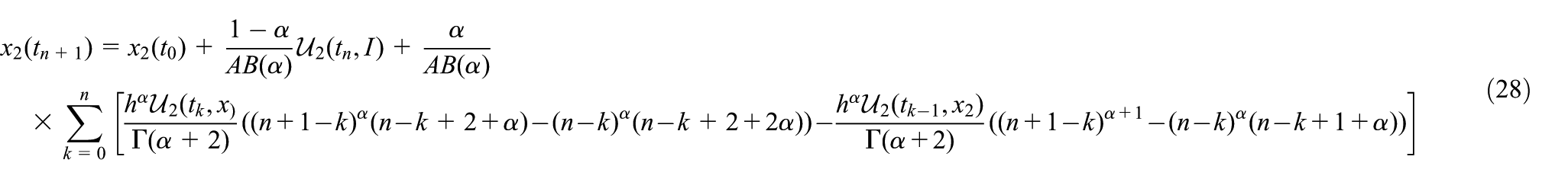
and
The numerical scheme presented for the model (23) is used further to obtain the numerical results by considering the fractional parameter
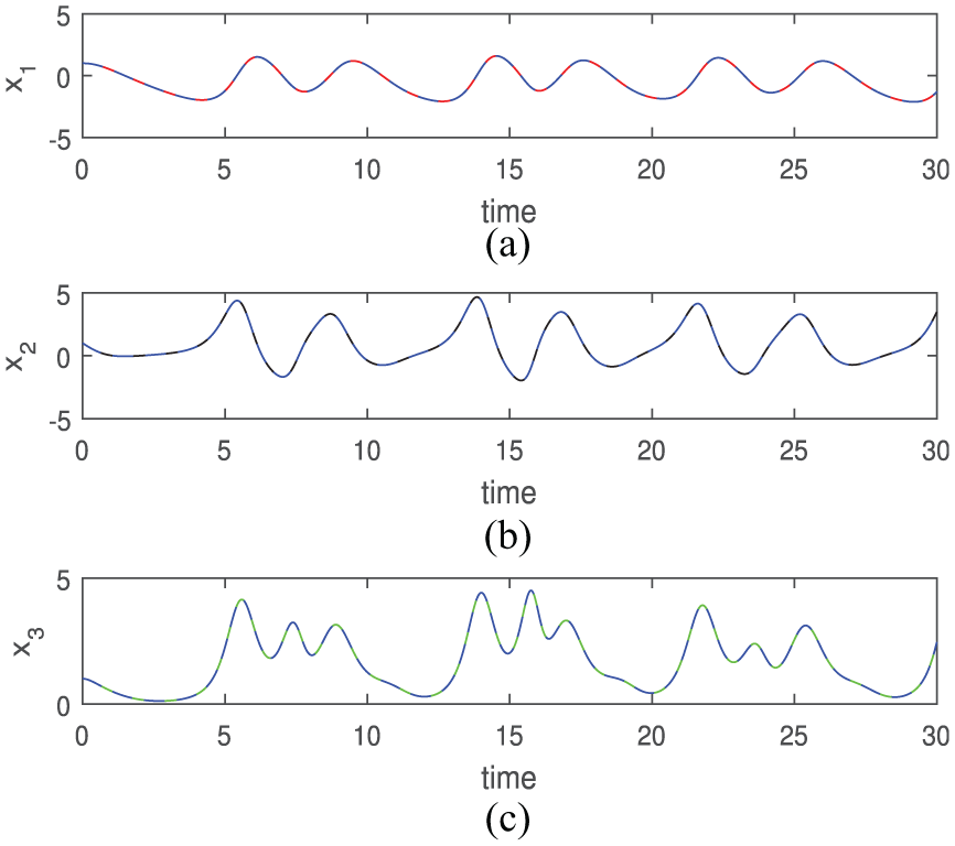
Considering the Atangana–Baleanu model (23), with α = 1: (a) state variable x1, (b) state variable x2 and (c) state variable x3.
Considering the Atangana–Baleanu model (23), with α = 0.95: (a) state variable x1, (b) state variable x2 and (c) state variable x3.

Considering the Atangana–Baleanu model (23), with α = 0.90: (a) state variable x1, (b) state variable x2 and (c) state variable x3.

Considering the Atangana–Baleanu model (23), with α = 0.85: (a) state variable x1, (b) state variable x2 and (c) state variable x3.

Considering the Atangana–Baleanu model (23), with
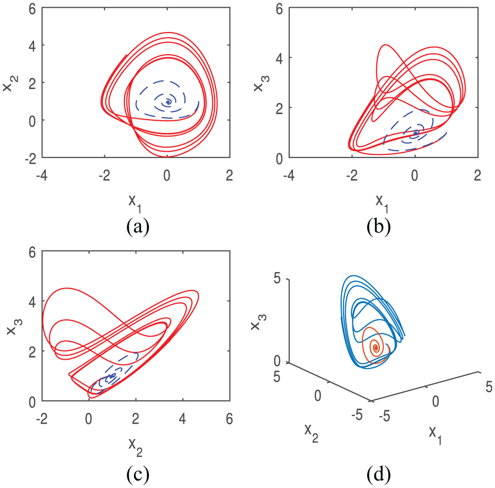
Considering the Atangana–Baleanu model (23), with α = 0.95, where the model shows chaotic attractor: (a) Phase portraits (x1-x2 plane), (b) Phase portraits (x1-x3 plane), (c) Phase portraits (x2-x3 plane) and (d) 3D plot (x1-x2-x3 plane).
Considering the Atangana–Baleanu model (23), with α = 0.9, where the model shows chaotic attractor: (a) Phase portraits (x1-x2 plane), (b) Phase portraits (x1-x3 plane), (c) Phase portraits (x2-x3 plane) and (d) 3D plot (x1-x2-x3 plane).

Considering the Atangana–Baleanu model (23), with α = 0.85, where the model shows chaotic attractor: (a) Phase portraits (x1-x2 plane), (b) Phase portraits (x1-x3 plane), (c) Phase portraits (x2-x3 plane) and (d) 3D plot (x1-x2-x3 plane).
Comparison of Atangana–Baleanu and Caputo–Fabrizio model
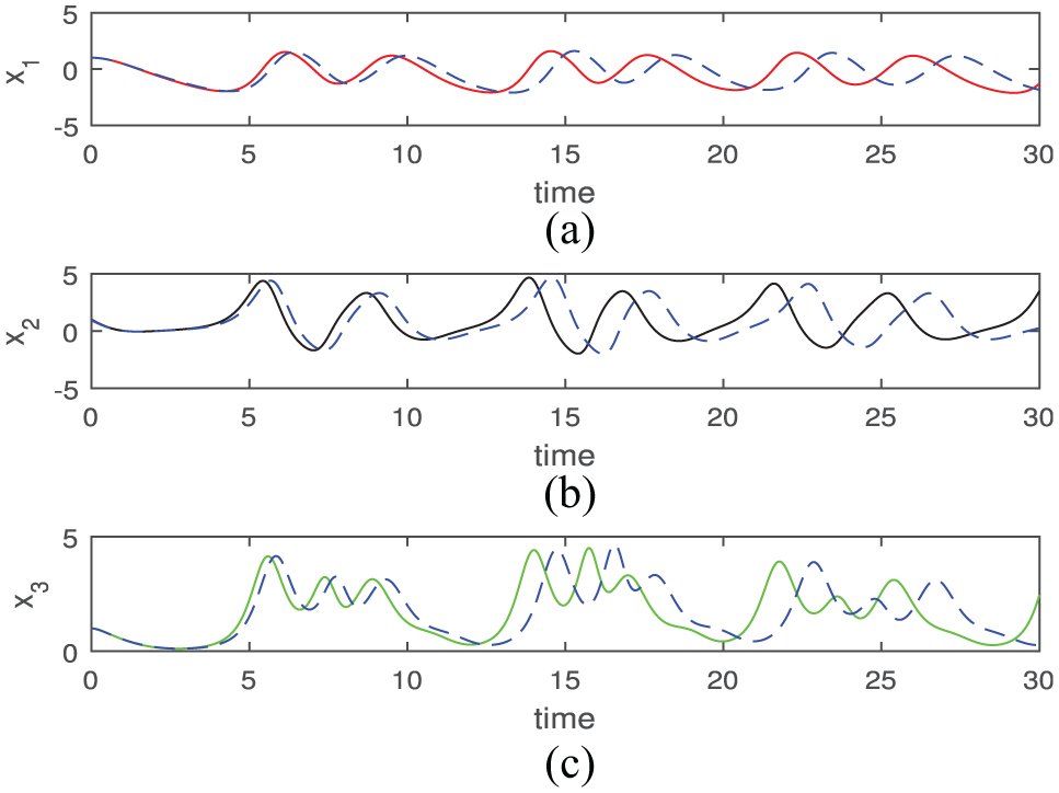
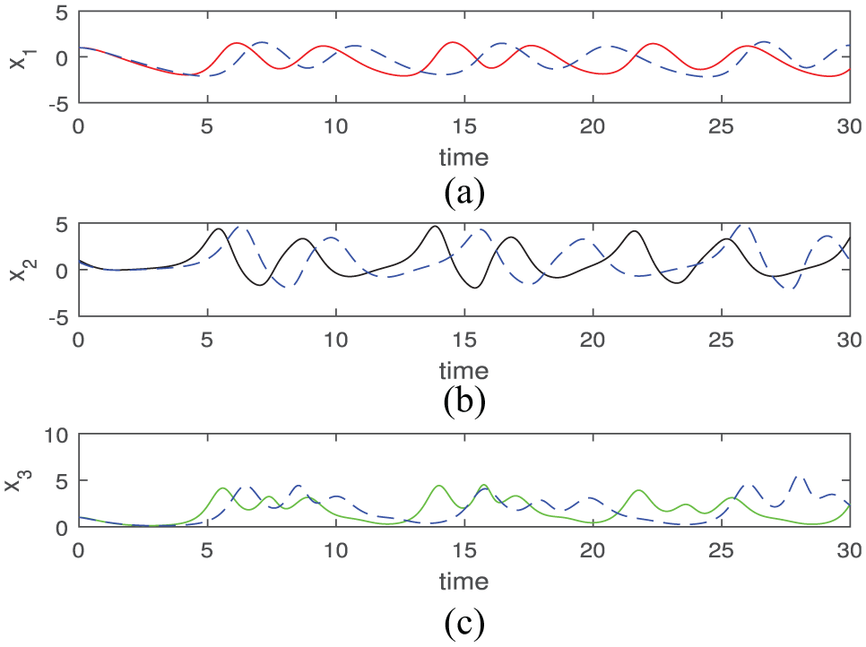
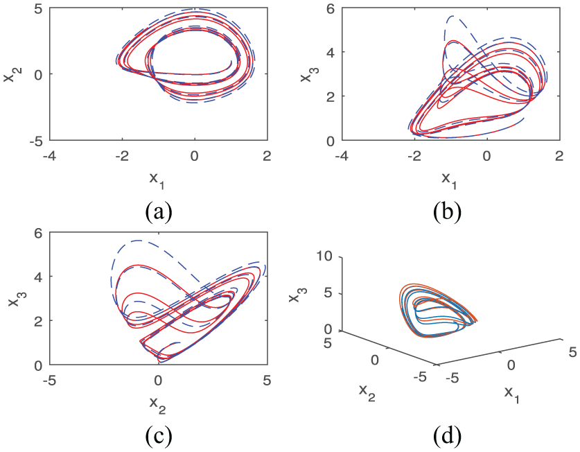
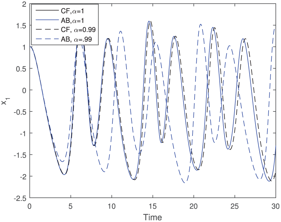
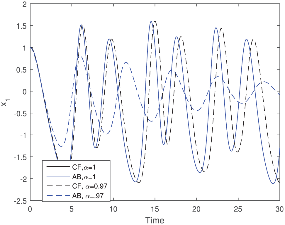
Here, we give the comparison of the fractional operators applied on the model (13) (see the Caputo–Fabrizio model (14) and the Atangana–Baleanu model (23)). We considered the numerical scheme presented for the Caputo–Fabrizio derivative model (14) and the Atangana–Baleanu model (23) and obtained the graphical results by taking the fractional-order parameter

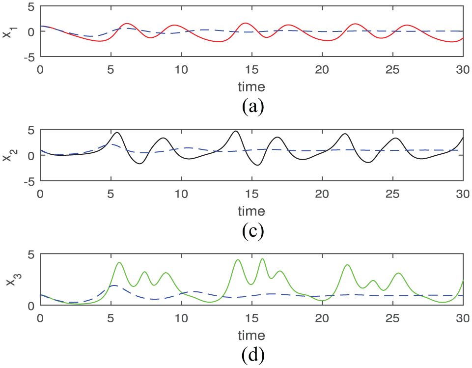
Considering the comparison graphs for the Caputo–Fabrizio model (14) and the Atangana–Baleanu model (23) when

Considering the comparison graphs for the Caputo–Fabrizio model (14) and the Atangana–Baleanu model (23) when

Considering the comparison graphs for the Caputo–Fabrizio model (14) and the Atangana–Baleanu model (23) when
Considering the comparison graphs for the Caputo–Fabrizio model (14) and the Atangana–Baleanu model (23) when

Considering the comparison graphs for the Caputo–Fabrizio model (14) and the Atangana–Baleanu model (23) when

Considering the comparison graphs for the Caputo–Fabrizio model (14) and the Atangana–Baleanu model (23) when
Considering the comparison graphs for the Caputo–Fabrizio model (14) and the Atangana–Baleanu model (23) when

Considering the comparison graphs for the Caputo–Fabrizio model (14) and the Atangana–Baleanu model (23) when

Considering the comparison graphs for the Caputo–Fabrizio model (14) and the Atangana–Baleanu model (23) when
Conclusion
We presented the dynamics of the new chaotic model in two fractional operators, the Caputo–Fabrizio operator and the Atangana–Baleanu operator. We discussed some of the basic properties of the model (13) earlier. Initially, we considered the new chaotic model and showed that the model is a chaotic attractor for the specified values and then we applied the Caputo–Fabrizio derivative to the new chaotic model (see equation (14)) and then applied the Atangana–Baleanu derivative and obtained the model (see equation (23)). Then, we presented the numerical approach for the solution of Caputo–Fabrizio model and for the Atangana–Baleanu model and obtained the graphical results by considering various values of the fractional-order parameter. Further, we considered both the models, that is, in Caputo–Fabrizio and the Atangana–Baleanu derivative sense and presented the comparison plots. The comparison plots were obtained by using the value assigned to the fractional-order parameter
Footnotes
Acknowledgements
The author is thankful to the anonymous referees and the handling editor for their careful reading and suggestions that improved the presentation of the article significantly.
Handling Editor: James Baldwin
Declaration of conflicting interests
The author(s) declared no potential conflicts of interest with respect to the research, authorship, and/or publication of this article.
Funding
The author(s) received no financial support for the research, authorship, and/or publication of this article.