
Abstract
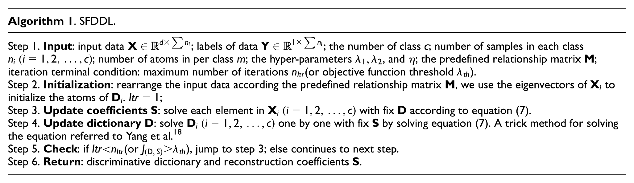
Vibration signals reflecting different kinds of machinery conditions are very useful for fault diagnosis. However, vibration signal characteristics are not the same for different types of equipment and patterns of failure. This available information is often lost in structureless condition diagnosis models. We propose a structured Fisher discrimination sparse coding–based fault diagnosis scheme to improve the feature extraction procedure considering both efficiency and effectiveness. There are three major components: (1) a structured dictionary for synthesizing the vibration signals that is learned by structure Fisher discrimination dictionary learning, (2) a tree-structured sparse coding to extract sparse representation coefficients from vibration signals to represent fault features, and (3) a support vector machine’s classifier on the features to recognize different faults. The proposed algorithm is verified on a standard bearing fault data set and a worm gear fault experiment. Test results have proved that the proposed method can achieve better performance with considerable efficiency and generalization ability.
Introduction
Bearings and gears are widely used in automobiles, machines, turbines, and mining equipments. Pre-emptive detection of bearings and gears failure is critical to the reliable operation of mechanical systems. 1 This can be achieved by making use of the information contained in vibration signals. The traditional basis representation algorithms such as fast Fourier transform (FFT), wavelet, 2 and variants of wavelet 3 are effective in dealing with vibration signals for fault diagnosis. However, the structural and discriminative information of vibration signals are not commonly used in the past. To overcome this limitation, new signal processing techniques have emerged to capture useful structural characteristics and discriminative information. 4 Recently, considerable attention has been paid to sparse coding representation–based techniques for vibration signals processing. 5 Sparse coding representation was first proposed for accurate signal reconstruction. 6 Representing a signal in decomposed forms involves the choice of a dictionary, which is a collection of elementary signals or atoms.7,8 In many tasks, the dictionary is fixed; for example, FFT and wavelets are special cases of signal representation based on fixed format dictionaries, but this is not sufficient for some complicated situations. A better approach is to learn a dictionary from the data itself, in which a sparse representation can be realized. 9
There are two practical ways to deal with the dictionary learning (DL) issue: using greedy pursuit algorithms10–12 and convex relaxation algorithms.13–15 For the first category of techniques, matching pursuit (MP)10,11 and orthogonal matching pursuit (OMP) 12 are the simplest approximate greedy algorithms. However, basis pursuit (BP) 14 and least absolute shrinkage and selection operator (Lasso) 15 are suitable to tackle the convex problem. Meanwhile, some other algorithms like the FOCal Underdetermined System Solver (FOCUSS) 16 were also developed. More details could be found in the previous studies.17–20 The shift invariant sparse coding (SISC) 21 algorithm was proposed in our previous research 22 that the training vibration signals are used to learn a dictionary, and the classification of new vibration signals was achieved by finding its sparse coefficients with respect to the activation distribution of the learned dictionaries.
However, these methods may not have taken advantage of the discriminative information within the data, especially when there are high correlations among the samples of different classes. Moreover, the efficiency and generalization ability of the algorithms are also important factors for fault diagnosis, while the computation of DL and sparse coding is complicated. Furthermore, how to resolve the signal based on the dictionary is another challenge for signal analysis. Hence, recently there are several attempts to include discrimination information in computing the dictionary and its coefficients.23,24 A Fisher discrimination–based dictionary learning (FDDL) scheme was proposed for image recognition. 25 The Fisher discrimination feature is inherited by sparse representation coefficients which present small within-class scatter and large between-class scatter. The sub-dictionary is constrained in order to preserve good reconstruction property for the target training class but poor for other classes. However, the Fisher discrimination features are only used to reflect the relationship between classes under data representation dimension. Even if the relationship between these classes is known, the inherent correlation is not considered between the classes.
In this article, we present a structured sparse representation fault diagnosis framework, which extends our previous work on sparse coding. 22 In the proposed framework, first, a structured dictionary is learned from training samples with labels by structured Fisher discrimination dictionary learning (SFDDL), where the dictionary atoms retain the corresponding class labels with a structured constraint. The atoms are arranged according to the correlation between classes—the more relevant the classes, the closer the atoms arranged in the dictionary. Then, the test samples are encoded by tree-structured sparse coding (TSSC) based on the learned dictionary. The tree structure enforces the faults with a hierarchical framework similar to a fault tree. The representation coefficients and its residual are both exploited in the final classification. Compared with our previous work in Liu et al., 22 which addressed the problem of how to efficiently generate features for vibration signals, we evaluate and validate our algorithm on a standard bearing faults database, and an experiment for worm gear faults is carried out.
The remainder of the article is organized as follows. Section “Structured Fisher discrimination sparse coding modeling” briefly describes the proposed fault diagnosis scheme, the SFDDL model, and the proposed TSSC model. In section “Case studies,” two experiments are described. The discussion of the results is presented in section “Discussion.” Finally, a conclusion is provided in section “Conclusion.”
Structured Fisher discrimination sparse coding modeling
To effectively reveal the structural information in vibration signals, the proposed method, structured Fisher discrimination sparse coding (SFDSC), adopts a machine learning algorithm which includes supervised DL and tree-structured coefficients solving, as shown in Figure 1. The vibration signals are acquired by the data acquisition system. Simultaneously, the fault information is recorded as the labels of the signals. Then, the vibration signals are processed, and details are given in sections “SFDDL” and “TSSC coefficients.”

Overview of the proposed methodology.
SFDDL
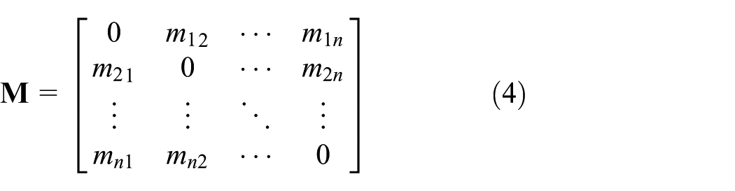
The unsupervised DL algorithm has achieved state-of-the-art results in image classification 26 and image reconstruction. 27 With the supervised or semi-supervised DL algorithms, labels of the training samples contain the class discrimination information that could lead to better classification results. 28 The Fisher discrimination criterion used in the classification maximizes the distances between two classes, while minimizes the distances within elements in each class. Discriminative DL includes two categories: one is the shared dictionary (SD) and the other is the partition dictionary (PD). All classes are learned by the SD, and the representation coefficients are discriminative. Only the correspondences of the subject class are used to learn a sub-dictionary of PD. However, the representative residual associated with each class can be used in the classification. At the same time, the representation coefficients are not required to be discriminative and are not further considered in the classification. 18 In addition, the correlation between classes is considered by a predefined relationship matrix.
Let

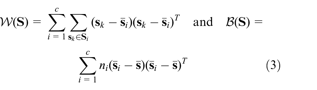
where
The reconstruction error of any training sample class

and we minimize this discriminative reconstruction error term.
Moreover, to increase the discrimination capability of dictionary
where
where

Following the study of Yang et al.,
18
we can define

and we also want to minimize the Fisher discrimination term. The variable
Considering the above discussion, we have the SFDDL model

Here, it is assumed that
The SFDDL has better discriminative capability; the learned dictionary based on the Fisher discriminative criterion essentially contains the distinguished information which has small within-class distance and large between-class distance. Furthermore, dictionary atoms are learned simultaneously in SFDDL, while methods based on BP13,21,22,29 learned atoms sequentially from one sample class to another. The SFDDL does not need to do a time-consuming convolution computation,21,22 and a batch processing method is employed in SFDDL instead of the tedious single cycle method. These considerations give SFDDL better generalization ability. The above-mentioned improvement will be confirmed in a practical application case presented in section “Case studies.”
TSSC coefficients
Recently, the tree structure sparse coding with group information about the features that yields a solution with grouped sparsity has received increasing attention in many areas including signal processing, machine learning, and statistical learning. For sparse coding, it is assumed that the groups of the inputs are available as prior knowledge, and it uses groups of inputs instead of individual input as a unit of variable selection.
30
Sparse coding achieved sparsity representation of the signal by applying the
In TSSC, the structure over the features can be represented as a tree with leaf nodes and internal nodes as clusters of the features. Such a regularization can help to uncover the structured sparsity, which is desirable for applications with some meaningful tree structures on the features. 32 In many applications, certain tree structures can naturally be used to represent features. But the resulting optimization problem is a lot more difficult to solve than Lasso and group Lasso, due to the complex regularization of the tree structures. Hence, tree structures are well applied in the field of fault diagnosis, for example, the fundamental concept in fault tree analysis is the translation of a physical system into a structured logic diagram (fault tree), where one specified top event of interest attribute to certain specified causes. 33 For a diagnostic system that knows the relationship between the faults, we can define a tree structure similar to the fault tree to represent the logic of faults. Here, we define a structured regularization with a predefined tree structure based on a group-Lasso penalty, where one group is defined for each node in an index tree. Figure 2 shows an example of the index tree.
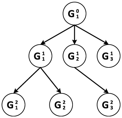
A sample of the index tree.
For an index tree T of depth d, we use
We define the tree-structured group regularization penalty term as

where
The penalized optimization problem associated with the tree-structured group regularization for a given learned dictionary is

where
In the model defined by equation (9), the value selected for the regularization parameter
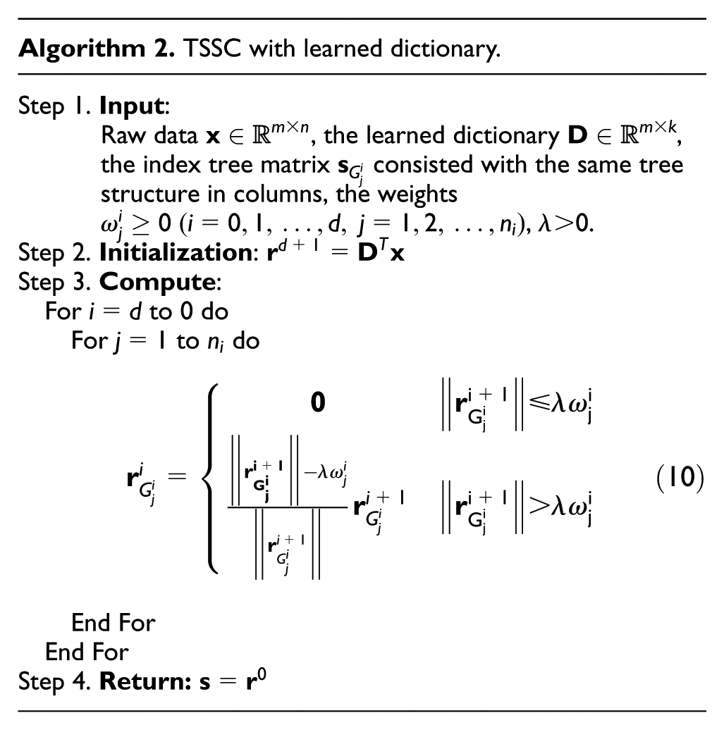
In the implementation of the TSSC algorithm, the first step is initiated by
Case studies
Bearing fault diagnosis experiment
The standard bearing fault vibration data were obtained from the bearing center of Case Western Reserve University (CWRU). 34 This data set had been referred as a benchmark. The vibration data were collected from the drive end ball bearing in a three-phase induction motor (Reliance Electric 2HP IQ PreAlert). The SKF 6205-2RS JEM deep groove ball bearing is tested with single point faults, which were seeded by electro-discharge machining. Fault diameters were 0.007, 0.014, 0.021, and 0.028 in. The fault locations were located on the inner race, the outer race, and the ball. An acceleration transducer was mounted on the motor housing at the driver end to acquire vibration signals. All signals were recorded at a sampling frequency of 12 kHz, for motor loads of 0, 1, 2, and 3 horsepower (hp0∼3), respectively. Samples without faults were also tested for the four levels of motor loads.
In this study, data sets were selected from the tests datasheet set out in Table 1. All raw data were segmented into a 1024-point sample without overlap, and signal edges were smoothed. At the same time, all samples were normalized to [−1, 1] with the mean value and standard deviation saved as two time-domain features. In this way, we obtained 118 samples for each set of faulty data, 1180 samples were obtained for each motor load (hp0∼3). Totally, 4720 samples with 10 classes of bearing date were used. Without loss of generality, half of the samples with motor load 0 hp were randomly selected to learn atoms, which are denoted by “*” in Table 1, while the remaining samples were used only for testing. The discriminability of sparse coefficients coding by the learned atoms was invoked as features for the bearing fault diagnosis. Meanwhile, the adaptability and generalization ability of the learned atoms was tested with the bearing data under motor load 1, 2, and 3 hp.
Bearing data set list.

These sets of samples are randomly split by half for learning atoms. The others are used for testing.
Atoms learning of bearing vibration signals by SFDDL
Faults on mechanical components can be indicated by vibration signals sensed from the machine. Vibration signals contain the fault information, the normal operational information, and the noise components. Therefore, effectively extracting the useful information of an abnormal condition is critical to machinery fault diagnosis. The proposal SFDDL method learns a discriminative dictionary from a small proportion of the vibration signals to capture the most information about the fault.
In our experiments, each atom with 1024 points has the same length of the samples from the original vibration signals. The number of atoms per class is 12, of which 10 classes of bearing fault data sets are learned. As a result, totally 10 sub-dictionary Ci (i =1, 2, …, 10) are generated, they make up an over-complete dictionary with 120 atoms, which are plotted in Figure 3. In this experiment, we choose the parameters as

where


The learned dictionary (atoms (N = 12) of each class are learned from the data set denoted in the subtitle).
Comparing each class of atoms in Figure 3 with others, there is an obvious difference between the normal condition (sub-dictionary C1(N)) and the others. Almost no impulses appear in the atoms of the normal condition. On the contrary, different degrees of impulses are distributed in the atoms of the inner race fault, the outer race fault, and the ball fault corresponding to the seriousness of fault diameter. The location and morphology of impulse variations are due to different mechanisms in generating impulses, which are the same as our previous work. 22
The reason for choosing the number of 12-atoms per class is a trade-off between computational cost (sum of learning and coding) and classification performance of fault diagnosis. Figure 4 shows the time consumed for learning the dictionary from half of the samples under motor load 0 hp with different number of atoms per class. The coding time for the remaining half samples under motor load 0 hp responding to the learned dictionary is also plotted. The learning time is approximately in linear proportion to the number of atoms per class, while the coding time is close to an S-curve. It means that the SFDDL DL time is increasing uniformly. But the TSSC coefficients coding time have a rapidly rising interval when the number of atoms per class is larger than 12

Time consumed on learning and coding with various number of atoms per class (half samples under motor load 0 hp for learning and the remaining half for coding).
Sparse coding of bearing vibration signals by TSSC
The proposal TSSC method is applied to solve sparse coding of vibration signals using the learned dictionary. In this experiment, the index of tree-structured group is shown in Figure 5. The root node is

Index of tree-structured group for bearing fault diagnosis.
For example, we randomly select one sample from one class. The result is shown in Figure 6. In the first row, the original vibration signals are plotted, where the trend has been removed and the amplitude is normalized to range [−1, 1]. It can be noticed that the normal conditions appear more stationary than the fault conditions which is composed of amplitude impulses in the signals. The sparse coding active coefficients are scattered in the second row. It shows that the TSSC produces is able to group sparse solutions. Furthermore, the group residuals and the group actives of the reconstructed are scattered in the third and fourth row. Similarly, they are normalized to range from −1 to 1. The result shows that, for the normal condition sample C1(N), the activation (non-zero coefficients) is exactly centered in the first group. The minimum value of residue and maximum value of activation are both discriminatively locating in class 1. Hence, normal condition could be classified easily using these features. In the same way, most samples could be distinguished correctly, although they have various distributions among classes. However, the inner race fault with fault diameter 0.014 in denoted as C3(I14) fails to be detected using this strategy. It could be explained that the signals are more complex and contain several different components of fault information which will be captured by different sub-dictionaries. In order to remove this defect, we can add some other features such as the time-domain features or frequency-domain features for the classification.

An example to illustrate the tree-structured sparse coding of different classes of vibration signals (randomly selected from testing half samples of hp0) with learned dictionary: the first row is the original vibration signal, the second row is the corresponding sparse coding coefficients, the third and fourth row are the normalized group residual values and normalized group activation values of the reconstruction for the original signal using different sub-dictionaries, respectively: (a) example of fault class C1–C5 and (b) example of fault class C6–C10.
Bearing faults diagnosis
As mentioned above, quadratic SVMs were implemented to classify the fault classes. At first, 70% samples in the test data under 0 hp motor load were used for 10-fold cross validation. Then, the remaining 30% samples were tested with the best accuracy validated model which was trained in the cross-validation phase. The results are shown in Figure 7. When the number of atoms per class (N) is smaller, the accuracy is lower, because there are only a few number of atoms that contain limited information about fault patterns. An upper bound about 90% can be found in both the cross validation and the test phase while N is larger than 12. This means that increase in the number of atoms cannot improve the performance of classification after a particular level. It can be explained that the over-complete dictionary had already acquired enough features of the samples’ fault pattern which had been defined in the task. Meanwhile, extra atoms will contain information that are not defined or not interested such as noise.

Classification accuracy rate of various numbers of atoms per class of bearing test data, under motor load 0 hp: 10-fold cross validation with 70% samples and test with the remaining 30% samples.
Worm gear fault experiment
Experimental setup
The experiment is conducted on a test bench as shown in Figure 8, and the type of the worm gearbox of the test rig is WPA (W-worm speed reduce, P-whole box structure, A-input shaft) 40 (ratio 1/10, number of threads 2, number of teeth 20, module 2.5 mm, lead angle 9°28′, pressure angle 20°, reference diameter of worm 30 mm) and driven by an alternating current (AC) servomotor. The loading is applied by another AC servomotor at 0 or 6 N m. Artificial faults (worm gear pitting, worm gear spalling, and worm gear broken as shown in Figure 9) are produced on the worm gear, and the vibration signal is sensed from the gearbox housing with sample frequency

Worm gear fault test platform.

Artificial worm gear fault specimens.
Worm gear faults diagnosis
The signals of different kinds of loadings and faults are acquired; as listed in Table 2, there are four classes of failures and two loading conditions for worm gear, and the raw vibration signals of worm gear under different conditions are shown in Figure 10. The signals have been divided into 1024 point segments as a sample. In total, 50 × 4 samples (50 samples per class) under free loading are used for DL, and another 50 × 4 samples under free loading and 50 × 4 samples under 6 N m loading are used for testing. The fault signal is processed according to the flowchart depicted in Figure 1. The parameters used for SFDDL is the same as the bearing case, except the number of atoms per class is 10, and the predefined relationship matrix is an identity matrix. Owing to every kind of failures has one degree of fault, the tree structure has two levels, one root node, and four children nodes in the second level.
Worm gear data set list.

These sets of samples are randomly split by half for learning atoms, the others are used for testing.

A set of raw vibration signals with faulted worm gear.
The learned dictionary is shown in Figure 11. It is worth noting that the learned dictionaries under fault conditions have significant low-frequency components in the atoms, but none in the normal condition. There are serious impact components in the atoms (such as atoms 2 and 6) under broken condition. It can be considered that these learned atoms contain the corresponding fault features. Hence, these atoms are able to represent the raw signals in the sparse model.

Learned dictionaries for worm gear faults by SFDDL.
The results for classification of the worm gear faults by SISC 22 and the proposed method SFDSC are shown in Table 3. In SFDSC, the accuracy for free loading is more than 96%, whereas it is about 88% at 6 N m loading. It also shows that the proposed method SFDSC has outperformed the SISC method in both cases.
Fault diagnosis accuracy for worm gear with SISC 22 and SFDSC.

SISC: shift invariant sparse coding; SFDSC: structured Fisher discrimination sparse coding.
Discussion
Generalization and robustness
In order to validate the adaptability and the generalization ability of the proposal model SFDSC, the variations of working loads in bearing data were utilized in tests. Based on the over-complete dictionary (12 atoms per class) which learned from half of the samples under motor load 0 hp by SFDDL, 20 feature vectors (10 group residual features and 10 group activation features) were extracted for the test-bearing data samples (totally
The classification accuracies for three cases of motor loads and different features are given in Table 4. For load hp1, the accuracies are higher than 87% in time-domain features sets, both on cross validation and test scenarios. More than 93% samples could be exactly distinguished under load hp2, while the average for load hp3 is about 92%. If we only focus on the fault categories such as N, I, O, and B, but not the particular values of fault diameters, then we have elevated results as follows: 100%, 97%, 98%, and 98% for hp0, hp1, hp2, and hp3, respectively. Furthermore, the misclassifications among categories are less than 3% for all loads status. It indicates that the proposed SFDSC has good generalization ability for bearing fault diagnosis problem.
Classification accuracy rates of SFDSC (dictionary learning set: half of hp0, 12 atoms per class. Validate and test set: hp0, hp1, hp2, and hp3; 70% for cross validation (CV), 30% for the test).
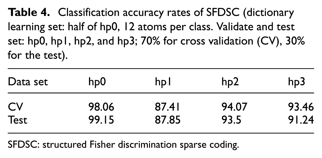
SFDSC: structured Fisher discrimination sparse coding.
Comparison with other algorithms
Using the same CWRU bearing set, Table 5 summarizes the classification results of different methods in the literatures and ours. As an abnormality detector, all techniques have a good performance, where nearly 100% faults could be identified. In the four category (N, I, O, and B) classification, the proposal method has the best result (100%) equivalent to international workshop on parsing technologies-support vector machine (IWPT-SVM). 35 Meanwhile, we have a generalization result about 98% of the unlearned data sets hp1, hp2, and hp3. For all 10 classes of fault diagnosis problem, we also have the best result 99.15%, which is similar to our previous work. 22 The generalization ability has been improved from 86.84% to 90.87%. This is because the SFDSC method takes full advantage of the hierarchical structure present in the bearing failure mode. The structured dictionary, which is learned by the proposed method, can better represent different types of bearing faults.
Comparisons with other methods based on CWRU bearing data set.

Bold values represent the results of the proposed algorithm in this paper.CWRU: Case Western Reserve University; IWPT-SVMs: international workshop on parsing technologies-support vector machines; SISC-LDA: shift invariant sparse coding-learning for dimensionality reduction and classification; HSSMC-SVM: hyper-sphere-structured multiclass-support vector machine; SFDSC-SVM: structured Fisher discrimination sparse coding-support vector machine.
The best results.
Using the first data set trained classifier in the article.
The average results.
The time cost for SISC 22 and SFDSC is compared in Table 6. The time was calculated under the same personal computer (PC) platform: Pentium® Dual-Core CPU E5800 @3.20 GHz, RAM 4.00 GB. It shows that SISC takes about 100 times more than SFDSC on the same scale of the dictionary. Even for the final used dictionary in SISC, the computation time is smaller than SFDSC. The time difference is greater than 100 multiples (10,455 s/98 s). It indicates that SFDSC has a better efficiency than SISC, which is very desirable for practice applications. There are two factors, batch processing without time-consuming convolution computation and the use of tree-structured index, that make SFDSC more efficient.
Computation time (seconds) for learning same size dictionary by SISC and SFDSC.

Bold values represent the results of the analysis cases in this paper.SISC: shift invariant sparse coding; SFDSC: structured Fisher discrimination sparse coding.
Number of atoms per class used in Liu et al. 22
Number of atoms per class used in this article.
Conclusion
In this article, we have presented a framework of sparse representation–based classification for machinery fault diagnosis. An SFDSC approach is applied to classify various types of faults in rolling element bearing. A structured dictionary with label is learned by structure Fisher discrimination DL, whose sub-dictionaries have discrimination ability: smaller within class dissimilar and larger distance between classes. The signal mean value and standard deviation are introduced to combine with the tree group structured sparse coding coefficients for fault diagnosis, and experiments have demonstrated that the classification of the SVMs is accurate. Furthermore, experimental results are also compared with previously published results using the same bearing data set. It shows that the performance of the proposed method is better than many state-of-the-art bearing fault diagnosis methods. Moreover, this approach can provide more generalization ability and higher efficiency. Some limitations are found in structure Fisher discrimination DL, such as the need for labeled samples for DL as well as the relationship of faults to predefine the tree structure. Notwithstanding the limitations, the effect of parameters based on empirical presumption on the final results is not obvious. Future works should seek a semi-supervised or unsupervised DL algorithm in which unlabeled samples could be used.
Footnotes
Academic Editor: Francesco Massi
Declaration of conflicting interests
The author(s) declared no potential conflicts of interest with respect to the research, authorship, and/or publication of this article.
Funding
The author(s) disclosed receipt of the following financial support for the research, authorship, and/or publication of this article: This research is supported by the National Natural Science Foundation of China (Grant no.51305258, 51275290, and 11202125) and National Key Technology R&D Program (2014BAD08B01, 2015BAF11B01).