Sage Journals: Discover world-class research

Abstract

With the wide application of intelligent equipment in modern industrial production, it is particularly important to study how to intelligently sense the faults of rotating machinery, improve the diagnosis efficiency and enhance the interpretation ability of the diagnosis process. Although the traditional 1-D CNN performs well in fault diagnosis, it has limitations in capturing subtle changes and complex patterns of fault signals, and its interpretability needs to be improved. Therefore, based on the improved ELCNN model, this paper discusses its diagnosis mechanism in depth, aiming at providing a new idea for intelligent fault diagnosis of rotating machinery. The functions of convolutional layer and S-GAP layer in ELCNN are studied and analyzed. Through single-layer linear convolution, ELCNN can adaptively learn the frequency domain features of the signal and realize the lightweight of the model. At the same time, the S-GAP layer enhances the ability of ELCNN to capture the main peak frequency of fault signals through feature sparseness. The experimental results show that the accuracy of ELCNN in frequency domain feature extraction is more than 80 %. The main peak frequency extracted can effectively help engineers understand the basis of model judgment and improve the reliability of the model.

Keywords

Fault diagnosis interpretability feature extraction diagnosis mechanism

Introduction

With the intelligent development of equipment, it is of great significance to study how to intelligently perceive the running state of rotating machinery such as bearings and gears, so as to find faults as soon as possible and avoid losses.^1,2 There are many methods to obtain fault signals, among which vibration signals are the most widely used.

The diagnosis process based on vibration signal analysis includes signal feature learning, state feature selection and transformation, fault pattern recognition, etc. There are three main ways to realize the above process: model-based fault diagnosis method, signal characteristic transformation and decomposition-based fault diagnosis method and knowledge-based fault diagnosis method.³

Model-based fault diagnosis refers to inferring the fault state by using the established data models and data analysis technology, such as RTSMFFDE-HKRR,⁴ stochastic resonance system in strongly coupled Duffing-Van der Pol oscillators,⁵ Digital Twin system,⁶ and so on. The advantage of this method is that it does not need extra hardware to realize fault detection, but it is extremely difficult to accurately model mechanical systems working in complex environment.

The methods based on signal feature transformation and decomposition are mainly to extract signal features through some feature transformation and decomposition methods, and analyze the types and trends of signals, such as Fourier transform (FT),⁷ wavelet transform (WT),⁸ variational mode decomposition (VMD),⁹ and so on. These methods are based on the state information released by the mechanical equipment during operation,¹⁰ and it is not necessary to establish a systematic mathematical model. However, they lack the ability to diagnose potential failures at an early stage.

Knowledge-based fault diagnosis methods diagnose and locate faults through knowledge of concepts and processing methods, such as expert systems based on existing knowledge,¹¹ fault trees,¹² and data-driven neural networks.¹³ Diagnostic methods based on existing knowledge have high requirements on the professional knowledge reserve of the diagnostician and do not have incremental or adaptive learning ability.¹⁴ Data-driven neural networks, especially the intelligent diagnosis method based on machine learning (ML), adaptively extracts knowledge from historical data and predicts the health status of machinery, reducing dependence on experts and experience, mainly including shallow models and deep models.

Shallow models, such as ML-based K-nearest neighbors (K-NN),¹⁵ artificial neural networks (ANN),¹⁶ and support vector machine (SVM),¹⁷ cannot extract complex fault features, and many aspects of the diagnosis process need human participation.¹⁴ The deep model based on deep learning (DL) has more complicated nonlinear expression ability and end-to-end learning ability, which makes the prediction of fault diagnosis model more accurate, such as autoencoder (AE),¹⁸ restricted Boltzmann machine (RBM),¹⁹ convolutional neural network (CNN),²⁰ and recurrent neural network (RNN).²¹ Among them, the one-dimensional convolutional neural network (1-D CNN) has obvious performance advantages. This is due to:

(1) Compared with AE and its variants, CNN has the ability of end-to-end adaptive learning, which is especially suitable for optimizing all link of fault diagnosis to improve the intelligent level of diagnosis.

(2) Compared with RBM and RNN, CNN has shorter training time and more effective learning through parallel operation of convolution.

(3) Compared with 2-D CNN, which takes image information as the network input (without mining the deep features of the signal), 1-D CNN takes one-dimensional time domain state signal as the network input, which has strong feature extraction ability.

Therefore, fault diagnosis based on 1-D CNN has been widely studied.^22–24 For example, Vo et al.,²¹ Chang et al.,²⁵ and Alsumaidaee et al.²⁴ obtain the spatial and temporal characteristics of signals by combining 1-D CNN, Long Short-Term Memory (LSTM), or Gated Recurrent Unit (GRU). However, the above-mentioned RNN variants still have some problems, such as high computational complexity, long training time, sensitivity to hyperparameters and poor interpretability. Zhang et al.²² and Swetapadma et al.²⁶ use data probability density and spectral entropy to provide input for convolutional layer, but they do not bring feature extraction process into the fault diagnosis process to achieve global optimization. Li et al.²⁷ and Kim et al.²⁸ used Class Activation Mapping to visualize the frequency domain features concerned by 1-D CNN, but did not interpret the working mechanism of the model in depth.

The above research mainly focuses on the fault diagnosis performance of 1-D CNN. Why does it have such excellent adaptive feature extraction ability? In the process of sample learning, what characteristics did it learn from the sample? How to reduce the characteristic dimension of vibration signal sample? The research on the problems of … etc. is very limited. The in-depth study of its feature extraction and fault diagnosis mechanism is of great value for inspiring people to understand the characteristics of the vibration signals of rotating machinery, thus improving the structure and parameters of 1-D CNN more pertinently, and guiding and strengthen the learning of 1-D CNN.

In the previous paper, the author proposed an interpretable lightweight convolutional neural network (ELCNN),²⁹ which has good performance. In order to meet the above challenges, this paper further discusses the network structure and fault diagnosis mechanism based on public data sets on the basis of ELCNN. The main work is as follows:

(1) This paper expounds the theoretical basis of ELCNN, and analyzes its theoretical relationship with traditional signal decomposition methods such as FT and WT.

(2) The fault features identified by ELCNN are extracted, and the frequency conversion mode and vibration waveform structure learned in the convolutional layer and S-gap (Square Global Average Pooling) layer are analyzed.

(3) Exploring the fault diagnosis mechanism of ELCNN can enlighten people’s understanding of model feature extraction, feature transformation and pattern recognition mechanism.

The structure of this paper is as follows: In section “Improved ELCNN for vibration diagnosis of rotating machinery,” the theoretical background of the improved ELCNN is introduced. In section “Analysis of feature extraction transformation results of ELCNN,” the features of the transform extracted by ELCNN are analyzed. In section “Analysis of the diagnosis mechanism of ELCNN,” the diagnosis mechanism of ELCNN is studied. In section “Summary and prospect,” the main work of this paper is summarized and future research is prospected.

Improved ELCNN for vibration diagnosis of rotating machinery

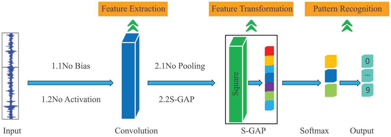
As shown in Figure 1, the ELCNN model I mentioned in my last paper has a significant improvement in model structure compared to the traditional 1-D CNN model. The model does not include bias, activation and pooling operations, and compresses the number of convolutional layers. Feature extraction and feature transformation are realized through single-layer linear convolution and S-GAP layer. The structural parameters of the network are shown in Table 1. As shown in Table 2, when the convolution kernel size is 16 and the number is 10, the diagnostic performance of ELCNN is the best, and the resource consumption is the least.

Figure 1.

Comparison of (a) traditional 1-D CNN and (b) improved ELCNN network structure.

Table 1.

Network structure of ELCNN.

No.	Layer type	Kernel size	Kernel number	Output size
1	Input	—	—	1 × 4096
2	Conv	16 × 1	10	10 × 4096
3	S-GAP	—	—	10 × 1
4	Softmax	10	1	10

Table 2.

Diagnostic performance of ELCNN under different hyperparameters. Among them, the diagnostic performance of the model is the best under the condition of red zone, which is 100.

Single-layer linear convolution

In order to realize the lightweight and interpretability of 1-D CNN, ELCNN draws lessons from the traditional linear convolution (LC), and removes unnecessary and redundant feature extraction links while retaining the time-frequency features of vibration signals as much as possible. LC is an important method of vibration signal feature transformation, which has a solid theoretical basis. It is a description of the input-output relationship of linear time-invariant systems in the time domain.³⁰ It is defined as follows.

\begin{matrix} y (k) = \sum_{n = 0}^{N - 1} x (n) h (k - n) = x (n) * h (k - n), \\ k = 0, 1, . . ., N - 1 \end{matrix}

(1)

where $x (n)$ is the input of the system, $h (k - n)$ is the unit impulse response of the system under the action of unit impulse, * is the linear convolution operation, and $k$ is the position index.

The traditional FT and WT are linear convolutions in essence. Among them, the Discrete Fourier Transform³¹ is the most basic signal analysis method. It transforms the signal from the time domain to the frequency domain, and then studies the spectrum structure and transformation law of the signal. The specific transformation formula is as follows.

y (k) = \sum_{n = 0}^{N - 1} x (n) e^{- j 2 π \frac{nk}{N}} = x (n) * e^{- j 2 π \frac{nk}{N}}; k = 0, 1, 2, . . ., N - 1

(2)

where $e^{- j 2 π \frac{nk}{N}}$ is the basis function of FT. Unlike FT, which can only obtain frequency domain information, WT can obtain both time domain and frequency domain information.³² The formula is as follows.

\begin{matrix} y (a, b) = \sum_{n = 0}^{N - 1} x (n) ϕ (\frac{n - b}{a}) = x (n) * ϕ (\frac{n - b}{a}); \\ a > 0, - \infty < b < \infty \end{matrix}

(3)

where $ϕ (\frac{n - b}{a})$ is the wavelet basis function, $a$ is the scaling factor, and $b$ is the translation factor.

FT is a fixed basis, and only global frequency domain information of the signal can be obtained. Through scale transformation and displacement transformation, WT can get higher resolution frequency domain information in time domain. However, the above two time-frequency analysis methods are based on the basis functions selected by human experience, and the 1-D CNN convolution kernel (basis function) is obtained based on sample adaptive learning,³³ which is defined as follows.

\begin{matrix} y (k) = f (\sum_{n = 1}^{N - 1} ω_{n} x_{k + n} + b) = f (ω_{n} * x_{k + n} + b); \\ k = 0, 1, . . ., N - 1 \end{matrix}

(4)

where $x$ , $ω$ , $b$ , and $f (\cdot)$ are the input signals, weight, bias, and activation function of the 1-D CNN convolutional layer.

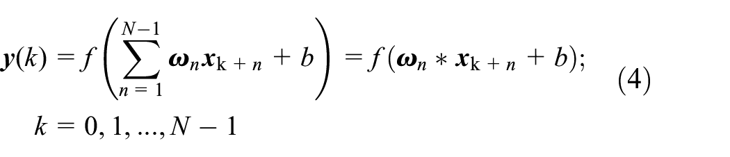
From the equations (1) to (3), it can be seen that there is no nonlinear mapping such as bias and activation in signal feature extraction methods such as FT and WT. Inspired by the above linear convolution, the proposed ELCNN removes bias and activation functions, and compresses the number of convolution layers to 1 layer, thus realizing a single-layer linear convolution. The ELCNN formula is defined as follows.

y (k) = ω_{n} * x_{k + n}; k = 0, 1, . . ., N - 1

(5)

where $ω_{n}$ is the weight of the convolutional layer and $x_{k + n}$ is the input signal of the convolutional layer.

The improved 1-D CNN model is still a convolutional neural network, because the essence of the neural network is not whether there is activation and bias, but whether the feature extraction ability of the model is based on sample learning. The convolution kernel is based on sample adaptive learning, which is beneficial to pattern recognition (fault classification). This is the most significant difference between the traditional linear convolution method and the proposed single-layer bitwise linear convolution.

Feature transformation layer S-GAP

The essence of pooling is to reduce the dimension of the input signal and restrain the over-fitting of training. However, the pooling operation tends to suppress broadband low-amplitude fault features (such as average pooling) or discards them (such as maximum pooling), thus reducing the model diagnosis accuracy.³⁴ As shown in Figure 2, average pooling and maximum pooling not only weaken the frequency domain characteristics of the signal (the green box part above 100 Hz in the figure), but also introduce the pseudo frequency components (the green box part below 100 Hz in the figure).

Figure 2.

Influence of the pooling layer on the time domain characteristics of the signal: (a) average pooling and (b) maximum pooling.

Although the traditional GAP overcomes the shortcomings of the fully connected layer parameter redundancy and the inability to maintain the spatial structure, and realizes the feature positioning ability, it cancels the positive and negative signals, weakens the signal characteristics, and reduces the classification effect of the model.

In order to solve the above two problems, ELCNN draws lessons from the feature selection link of the traditional fault diagnosis process and uses S-GAP to select the envelope from the time domain signal. The envelope spectrum is essentially a process of feature selection (feature sparsity), which emphasizes the main peak frequency in a frequency band and ignores the detailed features.

S-GAP squares the original signal first, then carries out GAP, and finally selected the envelope similar to the upper envelope and Hilbert envelope to realize the sparse characteristics of the vibration signal and improve the generalization ability of the model. This is mainly based on.

(1) The vibration signal is a one-dimensional sequence normalized to 0–1. The square operation can make the larger value of 0–1 larger and the smaller value smaller, expand the peak ratio and further highlight the main peak frequency.

(2) S-GAP has the ability of feature location, which can quickly lock the local peak feature, while square can overcome the positive and negative offset problem brought by the original GAP.

Based on the above improved strategy, ELCNN proposes an interpretable lightweight CNN, that is, signal feature extraction is realized by single-layer bitwise linear convolution, and feature sparsity of input signal is realized by S-GAP layer. The subsequent part of this paper will verify the effectiveness of the above strategies through experiments.

Analysis of feature extraction transformation results of ELCNN

In order to analyze and improve the feature extraction and transformation rules of ELCNN, this section analyzes the time domain and frequency domain features learned from convolution layer and S-GAP layer based on the public data set and combined with the fault features of the bearing inner ring and outer ring.

Sample source and classification

The signal samples come from the single conditional bearing data set of Case Western Reserve University (CWRU) and the multi-conditional bearing data set of Xi’an Jiao Tong University (XJTU).

The experimental platform of the CWRU single working condition bearing data set is the motor drive system, which is mainly composed of motor, torque sensor/decoder, power tester, etc.³⁵ The model of the drive end bearing is SKF 6205, and the bearing components are inner ring (IR), outer ring (OR), and balls (B). The working condition of the bearing is a motor load of 0 horsepower and a rotation frequency of 29.95 Hz. The experimental data is the vibration acceleration signal of the faulty bearing collected by the acceleration sensor, and the sampling frequency is 12 kHz. As shown in Table 3, the signal samples include IR, OR, and B faults, and the damage degree of each fault is 007, 014, and 021, respectively. To improve the availability of data and avoid contingency, signal samples are divided at equal intervals. One thousand five hundred samples are sampled for each fault type, and the ratio of samples included in the training set, verification set, and test set is 7:1:2.

Table 3.

Description of CWRU data set, including nine faults in three categories.

Fault	Rotational frequency (Hz)	Fault diameter (inch)	Class labels	Number of samples
				Training	Validation	Test
Normal	29.95	—	0	1050	150	300
B007	29.95	0.007	1	1050	150	300
B014	29.95	0.014	2	1050	150	300
B021	29.95	0.021	3	1050	150	300
IR007	29.95	0.007	4	1050	150	300
IR014	29.95	0.014	5	1050	150	300
IR021	29.95	0.021	6	1050	150	300
OR007	29.95	0.007	7	1050	150	300
OR014	29.95	0.014	8	1050	150	300
OR021	29.95	0.021	9	1050	150	300

The experimental platform of the XJTU multi-condition bearing data set is Spectra Quest, and the bearing model is NSK6203.³⁶ The bearing damage is a single-point damage processed with a grinding pen. The load of the bearing motor is 0 horsepower, and there are three kinds of rotating frequencies, which are 19.05, 29.05, and 39.05 Hz, respectively. The experimental data comes from the piezoelectric acceleration sensor, and the sampling frequency is 25.6 kHz. As shown in Table 4, the signal samples include Normal, IR, and OR faults, and the damage of each fault has three levels: mild, moderate, and severe. The preprocessing of signal samples is consistent with the CWRU.

Table 4.

Description of XJTU data set, including three kinds of rotation frequencies, three kinds of damage degrees and two kinds of faults, with 18 cases in total.

Fault	Rotational frequency (Hz)	Degree of injury	Class labels	Number of samples
				Training	Validation	Test
Normal	39.41	—	0	1050	150	300
IR1	19.07	Mild	1	1050	150	300
IR2	19.07	Moderate	2	1050	150	300
IR3	19.07	Severe	3	1050	150	300
OR1	19.07	Mild	4	1050	150	300
OR2	19.07	Moderate	5	1050	150	300
OR3	19.07	Severe	6	1050	150	300
IR1	29.05	Mild	7	1050	150	300
IR2	29.05	Moderate	8	1050	150	300
IR3	29.05	Severe	9	1050	150	300
OR1	29.05	Mild	10	1050	150	300
OR2	29.05	Moderate	11	1050	150	300
OR3	29.05	Severe	12	1050	150	300
IR1	39.41	Mild	13	1050	150	300
IR2	39.41	Moderate	14	1050	150	300
IR3	39.41	Severe	15	1050	150	300
OR1	39.41	Mild	16	1050	150	300
OR2	39.41	Moderate	17	1050	150	300
OR3	39.41	Severe	18	1050	150	300

Analysis of ELCNN feature extraction transformation results based on CWRU sample set

To study the results of ELCNN feature extraction and transformation, the inner and outer ring faults of CWRU are selected as experimental samples, and the time domain features, frequency domain features and input signals (Raw signals) concerned by the convolutional layer and S-GAP layer are compared and analyzed.

(1) IR fault

The rotation frequency of CWRU is 29.3 Hz, the IR fault is 161.2 Hz and the cage fault is 17.6 Hz. As shown in Figure 3, the impact characteristics of IR fault are obvious, and the S-GAP layer focuses on the peak characteristics, which can capture the signal envelope sensitively.

Figure 3.

Time domain waveform of IR014 learned by the (a) convolutional layer and (b) S-GAP layer.

As shown in Figure 4, the convolutional layer focuses on the global frequency domain characteristics of the signal, while the S-GAP pays more attention to the low-frequency characteristics of the signal.

Figure 4.

Spectrum of IR014 learned by (a) convolutional layer and (b) S-GAP layer.

As shown in Figure 5, the convolutional layer pays little attention to the fault frequency characteristics, while S-GAP pays more attention to the rotation frequency and its frequency doubling, IR fault and its sideband. For example, S-GAP learned the third harmonic of the rotation frequency of 90.9 Hz, the IR fault of 161.2 Hz and the sideband of 131.9 Hz (161.2 − 29.3 = 131.9).

Figure 5.

Hilbert envelope spectrum of IR014 learned by (a) convolutional layer and (b) S-GAP layer.

Similarly, from Table 5, we can draw a conclusion similar to the above time domain and frequency domain diagram, that is, the signal features learned in the convolutional layer are closer to the signal spectrum, and the signal features learned in the S-GAP layer are closer to the Hilbert envelope spectrum.

(2) OR fault

Table 5.

Correlation coefficients between the output of the convolutional layer, the S-GAP layer and the IR014 fault in the time domain and frequency domain feature maps.

Output\Feature map	Value of correlation coefficient
	Time domain	Frequency spectrum	Envelope spectrum
Convolutional layer	0.77	0.9	0.049
S-GAP layer	0.00088	0.15	0.76

Different from the IR fault, the OR fault has no obvious impact characteristics. On the contrary, it presents more complicated comb signal modulation characteristics. In addition, the S-GAP layer described in Figure 6 captures the upper envelope of the OR fault OR014.

Figure 6.

Time domain waveform of OR014 learned by the (a) convolutional layer and (b) S-GAP layer.

In Figure 7, the convolutional layer focuses on the global frequency domain features of 0R014, while S-GAP focuses more on the low-frequency features of the signal.

Figure 7.

Spectrum of OR014 learned by (a) convolutional layer and (b) S-GAP layer.

The convolutional layer in Figure 8 does not pay attention to the characteristics of fault frequency, while S-GAP adaptively learns many new fault frequencies from OR014 faults. For example, the frequency doubling of cage fault is 35.2 Hz (17.6 × 2 = 35.2), the OR fault frequency is 108.5 Hz (actually 107.36 Hz) and the sidebands are 143.6 Hz (108.5 + 17.6 × 2=143.7) and 161.2 Hz (108.5 + 17.6 × 3 = 161.3). Similarly, a conclusion similar to that in Table 5 can be drawn from Table 6.

Figure 8.

Hilbert envelope spectrum of OR014 learned by (a) convolutional layer and (b) S-GAP layer.

Table 6.

Correlation coefficients between the output of the convolutional layer, the S-GAP layer and the OR014 fault in the time domain and frequency domain feature maps.

Output\Feature map	Value of correlation coefficient
	Time domain	Frequency spectrum	Envelope spectrum
Convolutional layer	0.76	0.94	0.019
S-GAP layer	0.036	0.0056	0.6

In summary, compared with the IR014 fault, the OR014 fault is more complex and the characteristic frequency is less obvious, but ELCNN learns the new feature frequency through the global learning of the spectrum by linear convolution and the adaptive learning of the envelope spectrum by S-GAP, so as to accurately identify and classify the fault.

Analysis of ELCNN feature extraction transformation results based on XJTU sample set

Based on the CWRU sample set, the feature extraction and transformation rules of ELCNN are analyzed, that is, the features learned in the convolutional layer are close to the spectrum, and the features learned in the S-GAP layer are close to the Hilbert envelope spectrum. To further verify the above conclusions, this section conducts similar experiments based on the IR and OR faults of the XJTU sample set.

(1) IR fault

The cage fault of XJTU is 17.6 Hz, and the IR fault is 196.3 Hz. In Figure 9, the IR fault impulse excitation is not obvious, but S-GAP also captures the IR1 envelope.

Figure 9.

Time domain waveform of IR1 learned by the (a) convolutional layer and (b) S-GAP layer.

From Figures 9 to 11 and Table 7, it can be seen that, similar to the CWRU fault, the XJTU IR fault features learned in the convolutional layer are close to the spectrum, and those learned in the S-GAP layer are close to the Hilbert envelope spectrum. ELCNN can also adaptively learn the IR fault features of XJTU. S-GAP strengthens the cage fault frequency of 17.6 and 202.2 Hz (the actual IR fault is 196.3 Hz), and weakens the modulation characteristic of 44.0 Hz.

(2) OR fault

Figure 10.

Spectrum of IR1 learned by (a) convolutional layer and (b) S-GAP layer.

Figure 11.

Hilbert envelope spectrum of IR1 learned by (a) convolutional layer and (b) S-GAP layer.

Table 7.

Correlation coefficients between the output of the convolutional layer, the S-GAP layer and the IR1 fault in the time domain and frequency domain feature maps.

Output\Feature map	Value of correlation coefficient
	Time domain	Frequency spectrum	Envelope spectrum
Convolutional layer	0.018	0.83	0.07
S-GAP layer	0.026	0.18	0.58

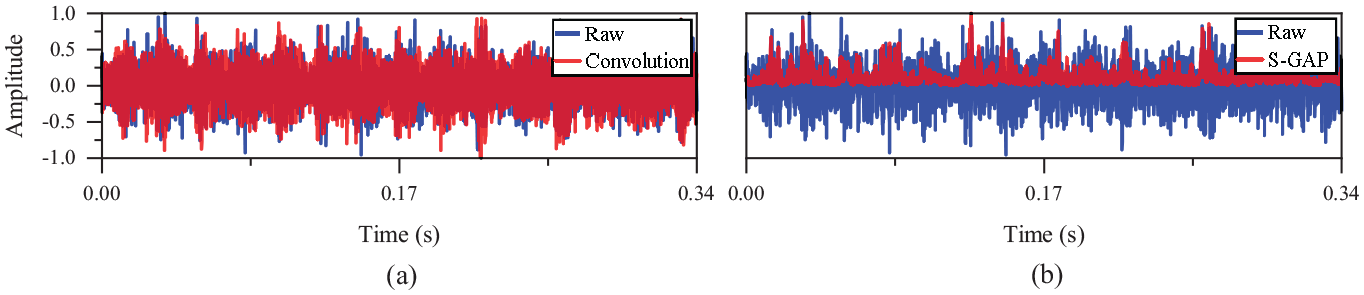
ELCNN feature extraction transformation rules similar to CWRU bearing fault can also be obtained from OR fault (Figures 12 to 14).

Figure 12.

Time domain waveform of OR1 learned by the (a) convolutional layer and (b) S-GAP layer.

Figure 13.

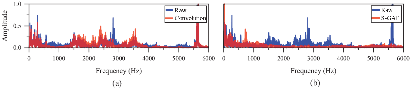
Spectrum of OR1 learned by (a) convolutional layer and (b) S-GAP layer.

Figure 14.

Hilbert envelope spectrum of OR1 learned by (a) convolutional layer and (b) S-GAP layer.

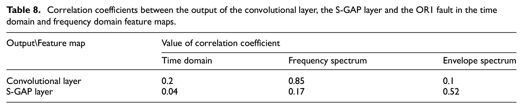
As shown in Figure 14 and Table 8, S-GAP learns many new fault frequency harmonics and sidebands. For example, it adaptively learns OR fault frequency and harmonics: 8.8 Hz (its frequency doubling is cage frequency 17.6 Hz), cage fault frequency doubling 35.2 Hz (17.6 × 2 = 35.2), rotation frequency 20.5 Hz (actual 19.07 Hz), OR fault frequency 117.2 Hz (actual 119.8 Hz), OR fault frequency doubling 240.4 Hz. For example, it adaptively learns OR fault sidebands: 111.3 Hz (119.8 − 8.8 = 111) with 8.8 Hz modulation, 90.9 Hz (111.3 − 20.5 = 90.8) and 131.9 Hz (111.3 + 20.5 = 131.8) with 8.8 Hz and 20.5 Hz modulation. It can be seen that compared with the IR fault in Figure 11, ELCNN learns more complex OR fault harmonics and sidebands through adaptive learning.

Table 8.

Correlation coefficients between the output of the convolutional layer, the S-GAP layer and the OR1 fault in the time domain and frequency domain feature maps.

Output\Feature map	Value of correlation coefficient
	Time domain	Frequency spectrum	Envelope spectrum
Convolutional layer	0.2	0.85	0.1
S-GAP layer	0.04	0.17	0.52

Analysis of the diagnosis mechanism of ELCNN

The improved ELCNN for vibration signals integrates the functions of signal feature extraction, feature selection and transformation, and fault pattern recognition in traditional fault diagnosis through adaptive learning based on signal samples (Figure 15). For example, single-layer linear convolution learns global spectral features, the S-GAP layer learns similar Hilbert envelope spectrum features, and the Softmax layer can realize pattern recognition. To explain the above phenomena, the internal working mechanism will be analyzed individually according to the above diagnostic links.

Figure 15.

Diagnosis process of ELCNN.

Feature recognition mechanism of convolutional layer

The learning ability of a single convolutional kernel (CK) is limited, and ELCNN uses multiple convolutional kernels to extract richer feature information. Figure 16 shows the fault features of rolling elements extracted by different convolutional kernels in the same convolutional layer in ELCNN. Among them, the second and fifth convolutional kernels mainly focus on low-frequency features (such as 161.2 Hz), while other convolutional kernels mainly focus on high-frequency features greater than 1000 Hz.

Figure 16.

Spectrum of feature maps learned by different convolutional kernels: (a) CK-1, (b) CK-2, (c) CK-3, (d) CK-4, (e) CK-5, (f) CK-6, (g) CK-7, (h) CK-8, (i) CK-9, and (j) CK-10, where Raw represents the input signal.

The differences in frequency characteristics focused on by different convolutional kernels are significant. Selvaraju et al.³⁷ proposed a gradient-weighted class activation map (Grad-CAM), and the formula is as follows.

L_{Grad - CAM}^{c} = ReLU (α_{k}^{c} A^{k})

(6)

where $α_{k}^{c}$ is the classification contribution (weight) of the k-th feature map of the one-dimensional vibration signal of category $c$ , and $A^{k}$ is the k-th feature map. The data in Table 9 is the contribution $α_{k}^{c}$ of the convolutional kernel to the classification results in equation (6). By weighting the feature maps learned by ELCNN using the above contributions, a CAM that is more conducive to classification can be obtained.

Table 9.

Contribution of each convolutional kernel to classification results.

No.	1	2	3	4	5	6	7	8	9	10
Contribution	0.33	0.36	−0.73	0.36	0.69	0.35	−2.79	0.36	0.54	0.53

Figure 17 shows the spectrum of different convolutional layer CAMs learned by different feature transformation methods. Compared with single-layer bitwise linear convolution (Figure 17(f)), 1D-CNN with bias (Figure 17(b)), activation function (Figure 17(c) and (d)) and multi-layer convolution (Figure 17(e)) can extract nonlinear features in the signal, but the drawbacks are also obvious.

(1) The useful features of the signal may be lost. As shown in Table 10, the feature map learned by the convolution with bias has a high correlation coefficient with Raw (discarding features with low correlation and retaining features with high correlation), but it is weak in learning the failure frequency of 161.2 Hz in Figure 18(a), which is often an important basis for fault classification. The reason why convolution with bias is poor in weak feature learning is that the essence of bias is to extract the local feature information in the signal and discard the information beyond the threshold through the bias parameter. For the vibration signal of rotating machinery, especially the early faults, its fault characteristics are often very weak, submerged in the normal vibration signal and even noise, and cannot be ignored.

(2) Pseudo features may be introduced. The activation function is a nonlinear function, which will lead to the deviation of the features learned by the convolutional layer, and may introduce pseudo-features that do not exist. For example, the activation functions Softsign and ReLU in the above image have a great influence on the learning of the model (correlation coefficient is less than 0.5). First of all, they introduce many nonlinear components, and there are deviations in the learning of low-frequency (frequency domain features less than 1000 Hz in Figure 17(c) and (d)) and high-frequency (3000–4000 Hz frequency domain features in Figure 17(c) and (d)) features. Secondly, they introduce pseudo-features, especially high-frequency features greater than 5000 Hz (Figure 17(c) and (d)), which are not present in the original signals.

(3) Too many network layers will cause unstable training and low computational efficiency. Traditional CNN often uses multi-layer convolution to extract richer features through high-order transformation, while multi-layer convolution often leads to complex network scale and large amounts of calculation. For example, the three-layer convolutional ELCNN-3 does not learn the low-frequency characteristics of the original signal (the frequency component less than 1000 Hz in Figure 17(e)), which is caused by unstable calculation caused by multi-layer convolution.

Figure 17.

Spectrum of CAMs in different convolutional layers learned by different feature transformation methods: (a) Raw, (b) Bias, (c) Softsign, (d) ReLU, (e) ELCNN-3, and (f) ELCNN-1.

Table 10.

Correlation coefficients between CAM and Raw in different convolutional layers learned by different feature transformation methods on spectral features, among which two red regions are better, and the correlation coefficients are greater than 0.9.

Figure 18.

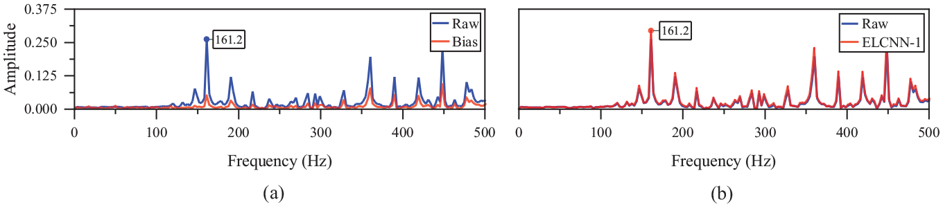
Spectrum of the convolutional layer CAMs learned by the (a) Bias and (b) ELCNN-1.

The significance of fault diagnosis is to find potential faults, that is, to find fault features through certain feature extraction and transformation methods, rather than using nonlinear high-order functions to infinitely approximate the input signal.

Inspired by the fact that FT, WT, and other signal feature extraction methods have no nonlinear mapping such as bias and activation, ELCNN-1 removes bias and activation functions and adopts single-layer linear convolution. Experiments show that the single-layer linear convolution of ELCNN-1 has the same strong frequency domain feature extraction ability as traditional linear convolution.

Feature transformation mechanism of S-GAP layer

The linear convolution of ELCNN has strong frequency domain feature extraction ability, but not all the detailed features are beneficial to classification. The model is too good in the frequency domain and may be over-fitting, which will affect its generalization performance.

The traditional 1-D CNN reduces the dimension by pooling operation to prevent over-fitting of the model. However, due to the limitations of its dimensionality reduction algorithm, broadband low-amplitude fault features are often suppressed (such as average pooling) or discarded (such as maximum pooling). ELCNN uses S-GAP (sparse operation) to select the signal envelope, highlight the main peak frequency and ignore the details, thus strengthening the fault characteristics.

Figure 19 shows the time domain waveforms of different envelopes. Compared with the feature extraction principles of Up Envelope and Hilbert Envelope, ELCNN uses S-GAP to sparse the features learned by linear convolution, where 1S-GAP represents the square of the output signal of the convolutional layer, 2S-GAP represents the quartic of the output signal of the convolutional layer, and 3S-GAP represents the octave of the output signal of the convolutional layer.

Figure 19.

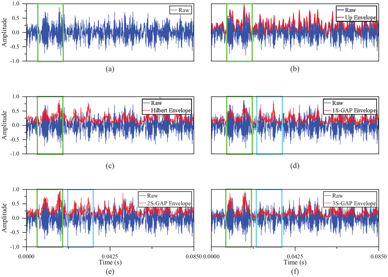
Time domain waveforms of different envelopes, in which the green box is the envelope of the reinforcement learning, and the blue box is the envelope of the weakening learning: (a) Raw, (b) Up Envelope, (c) Hilbert Envelope, (d) 1S-GAP Envelope, (e) 2S-GAP Envelope, and (f) 3S-GAP Envelope.

In Figure 19(b), Up Envelope learns the peak characteristics of the input signal, but it is relatively rough; in Figure 19(c), Hilbert Envelope learns the signal envelope more finely. The S-GAP shown in Figure 19(d) to (f) can learn similar Hilbert envelope amplitude characteristics, and square the output signal of the convolutional layer many times to suppress the invalid characteristics and noise characteristics, and highlight the peak characteristics more effectively (as shown in the blue box of 2S-GAP and 3S-GAP in Figure 19(e) and (f)).

The (b)–(f) of Figure 20 is the green box part of (a). Up Envelope of Figure 20(b) learned the fault sidebands of 161.2 Hz (108.5 + 17.6 × 3 = 161.3) and 131.9 Hz (161.3 − 29.3 = 132), of which 108.5 Hz is the OR fault, 17.6 Hz is the cage fault frequency and 29.3 Hz is the rotation frequency. Compared with the Up Envelope, the Hilbert Envelope in Figure 20(c) learns more sideband features, such as 96.73 Hz (131.9 − 17.6 × 2 = 96.7). Figure 20(d) to (f) are the S-GAP proposed in this paper. It can learn frequency features similar to Hilbert Envelope, and can more effectively suppress high-frequency features (especially the blue box part of 3S-GAP) through the multi-layer square, and extract more obvious low-frequency fault features (such as 120.2 and 178.8 Hz frequency components learned by 3S-GAP).

Figure 20.

Spectrum of different envelopes, where (b)–(f) is the frequency band below 500 Hz in the (a) green box, and the blue box of (d)–(f) is the frequency band weakened by S-GAP after multiple squared. (a) Raw, (b) Up Envelope, (c) Hilbert Envelope, (d) 1S-GAP Envelope, (e) 2S-GAP Envelope, and (f) 3S-GAP Envelope.

In summary, the S-GAP proposed in this paper can learn the frequency characteristics similar to the Hilbert Envelope, and it is easier to highlight the main peak frequency through multiple squares, and the fault signal can be effectively separated, which is conducive to the next pattern recognition (fault classification).

Pattern recognition mechanism of Softmax layer

Similar to the traditional signal processing method, the input signal is extracted by the feature extraction of the linear convolutional layer of ELCNN and the feature transformation of the S-GAP layer, and finally sent to the Softmax layer for pattern recognition. The whole training process is an iterative cycle, which is analyzed as follows.

(1) Learning feature maps. As shown in Figure 21, the ELCNN convolutional layer is continuously iteratively trained. After Epoch = 13, the variable values of the convolutional kernel are gradually stable, the model converges, and the convolutional layer learns the effective feature maps (Figure 17).

(2) Sparse feature maps. The S-GAP layer transforms the feature maps output by the convolutional layer through the square operation (Learn the envelopes of the feature maps in Figure 19) and obtains the sparse feature maps.

(3) Calculate classification confidences. The S-GAP layer transforms the sparse feature maps (FM) into the classification confidences of the feature maps in Figure 22(a).

(4) Perform pattern recognition. Through the fully connected layer learning of the Softmax layer, the classification confidences of different feature maps in Figure 22(a) are converted into the classification probabilities of different categories in Figure 22(b) (C1–C10, in which C8 has the highest classification probability), thus realizing pattern recognition.

Figure 21.

Iterative training results of convolutional kernel in the ELCNN convolutional layer, where the abscissa is the convolutional kernel variable sequence 1–16, and the ordinate is the convolutional kernel variable value.

Figure 22.

The classification confidence values of different feature maps and the classification probabilities of different categories: (a) confidence value and (b) classification probability.

ELCNN is a data-driven supervised learning model. It adjusts the parameters of the convolutional kernels through the backpropagation of errors and iterates the above process continuously. It is an end-to-end adaptive learning process. However, compared with the traditional 1-D CNN, the pattern recognition process of ELCNN has both similarities and differences.

(1) The recognition methods are the same. They all realize fault pattern recognition through Softmax.

(2) ELCNN first learns the frequency domain features of the signal with high similarity through linear convolution, then completes the feature sparsity through S-GAP (learns features similar to Hilbert envelope), and finally sends them to Softmax for pattern recognition. The traditional 1-D CNN uses nonlinear feature transformation methods, such as bias, activation function, pooling layer, and multi-layer convolution. Its diagnosis models are complex and unstable, which leads to deviations in learning characteristics.

Summary and prospect

Based on the CWRU and XJTU bearing data sets, the feature extraction and transformation results of ELCNN are studied, and its diagnosis mechanism is analyzed. The following conclusions have been drawn.

(1) The convolutional layer uses bitwise linear convolution with the signal, which is similar to the frequency decomposition of the signal in frequency domain analysis to extract frequency domain features. The optimized convolutional layer can learn rich frequency and amplitude variation patterns (correlation coefficients of spectral features >0.8), and the lightweight convolution is more helpful in achieving the optimal configuration of model size and parameters.

(2) By selecting the envelope characteristics of the signal, the S-GAP layer can more easily capture the peak and valley positions of the signal (correlation coefficients of Hilbert Envelope features >0.5), which is helpful for humans to understand the local structural characteristics of the vibration signal waveform and then understand the feature extraction process of the network.

In general, the bitwise linear convolutional layer extracts the basic features of the signal (global frequency domain and amplitude features), and the S-GAP layer extracts the complex features of the signal (frequency modulation and amplitude modulation features, local structure of the waveform). ELCNN, which adopts single-layer bitwise linear convolution, has the advantages of lightweight and interpretability. In future work, we can try to use ELCNN for fault detection of lightweight equipment such as drones, or as a high-performance classifier for generators such as GAN, to provide higher-quality fault samples for other models.

Footnotes

Acknowledgements

The authors thank the Case Western Reserve University (CWRU) and the Xi’an Jiao Tong University (XJTU) for the experimental data.

Handling Editor: Aarthy Esakkiappan

Author contributions

Concept and design: Jian Tang and Pengfei Pang, data collection and analysis: Jiancheng Gong, drafting of article: Yucheng He, critical revision of the article for important intellectual content: Jian Tang and Pengfei Pang, study supervision: Ting Rui. All the authors approved the final article.

Declaration of conflicting interests

The author(s) declared no potential conflicts of interest with respect to the research, authorship, and/or publication of this article.

Funding

The author(s) disclosed receipt of the following financial support for the research, authorship, and/or publication of this article: This study was supported by the National Natural Science Foundation of China (Grant No.: 51705531).

ORCID iDs

Jian Tang

Yuchen He

References

Sun

Cao

Wang

, et al. An interpretable anti-noise network for rolling bearing fault diagnosis based on FSWT. Measurement 2022; 190: 110698.

Zhang

Wen

Dong

, et al. A novel multiscale lightweight fault diagnosis model based on the idea of adversarial learning. IEEE Trans Instrum Meas 2021; 70: 1–15.

Peng

Xue

, et al. A survey on fault diagnosis of rolling bearings. Algorithms 2022; 15: 347.

Zhang

Jin

, et al. RTSMFFDE-HKRR: a fault diagnosis method for train bearing in noise environment. Measurement 2024; 239: 115417.

Zhang

Stochastic resonance in strongly coupled duffing and van der pol oscillators under trichotomous noise and bearing fault diagnosis. Fluct Noise Lett 2020; 19: 20500236.

Feng

Zhang

, et al. Digital twin-driven intelligent assessment of gear surface degradation. Mech Syst Signal Process 2023; 186: 109896.

Wen

Multilevel fine fault diagnosis method for motors based on feature extraction of fractional fourier transform. Sensors 2022; 22: 1310.

Cheng

Lin

, et al. Intelligent fault diagnosis of rotating machinery based on continuous wavelet transform-local binary convolutional neural network. Knowl Based Syst 2021; 216: 106796.

Feng

, et al. A fault information-guided variational mode decomposition (FIVMD) method for rolling element bearings diagnosis. Mech Syst Signal Process 2022; 164: 108216.

10.

Feng

Smith

Borghesani

, et al. Use of cyclostationary properties of vibration signals to identify gear wear mechanisms and track wear evolution. Mech Syst Signal Process 2021; 150: 107258.

11.

Patel

Upadhyay

SH.

Euclidean distance based feature ranking and subset selection for bearing fault diagnosis. Expert Syst Appl 2020; 154: 113400.

12.

Waghen

Ouali

M-S.

Interpretable logic tree analysis: a data-driven fault tree methodology for causality analysis. Expert Syst Appl 2019; 136: 376–391.

13.

Zhu

Jiang

, et al. Intelligent bearing fault diagnosis using PCA-DBN framework. Neural Comput Appl 2020; 32: 10773–10781.

14.

Liu

Zhou

Zhao

, et al. Fault diagnosis of rotating machinery under noisy environment conditions based on a 1-D convolutional autoencoder and 1-D convolutional neural network. Sensors (Basel) 2019; 19: 972.

15.

Qian

Sun

Wang

, et al. A weighted kNN fault detection based on multistep index and dynamic neighborhood scale under complex working conditions. IEEE Access 2023; 11: 49183–49192.

16.

Muhsen

Husin

Zolkepli

, et al. Enhancing NoC-based MPSoC performance: a predictive approach with ANN and guaranteed convergence arithmetic optimization algorithm. IEEE Access 2023; 11: 90143–90157.

17.

Biswas

Ray

Dey

, et al. Detection of simultaneous bearing faults fusing cross correlation with multikernel SVM. IEEE Sens J 2023; 23: 14418–14427.

18.

Cai

Song

Latent fault detection and diagnosis for control rods drive mechanisms in nuclear power reactor based on GRU-AE. IEEE Sens J 2023; 23: 6018–6026.

19.

Nedaei

Eskandari

Milimonfared

, et al. A bi-level line-line fault detection model for photovoltaic arrays using RBM-based automatic feature extraction. In: 2023 international conference on future energy solutions (FES), Vaasa, Finland, 12–14 June 2023, pp.1–6. New York, NY: IEEE.

20.

Song

Wang

Lai

, et al. On Bayesian optimization-based residual CNN for estimation of inter-turn short circuit fault in PMSM. IEEE Trans Power Electron 2023; 38: 2456–2468.

21.

T-T

Liu

M-K

Hsieh

C-L

. Hybrid 1D CNN-RNN network for fault diagnosis in induction motors using electrical signals. In: 2023 international conference on system science and engineering (ICSSE), Ho Chi Minh, Vietnam, 27–28 July 2023, pp.212–217. New York, NY: IEEE.

22.

Zhang

Pang

Zhao

, et al. A new method based on encoding data probability density and convolutional neural network for rotating machinery fault diagnosis. IEEE Access 2023; 11: 26099–26113.

23.

Qian

Qin

Luo

, et al. Deep discriminative transfer learning network for cross-machine fault diagnosis. Mech Syst Signal Process 2023; 186: 109884.

24.

Alsumaidaee

YAM

Paw

JKS

Yaw

, et al. Fault detection for medium voltage switchgear using a deep learning hybrid 1D-CNN-LSTM model. IEEE Access 2023; 11: 97574–97589.

25.

Chang

C-J

Chen

C-C

Chen

B-H

. Bearing fault diagnosis based on an advanced method: ID-CNN-LSTM. In: 2023 IEEE 6th Eurasian conference on educational innovation (ECEI), Singapore, 3–5 February 2023, pp.63–66. New York, NY: IEEE.

26.

Swetapadma

Shuvam

Behera

. A novel fault identification technique for transmission lines based on spectral entropy and one-dimensional CNN. In: 2023 fifth international conference on electrical, computer and communication technologies (ICECCT), Erode, India, 22–24 February 2023, pp.1–5. New York, NY: IEEE.

27.

Yao

Fan

, et al. An explainable one-dimensional convolutional neural networks based fault diagnosis method for building heating, ventilation and air conditioning systems. Build Environ 2021; 203: 108057.

28.

Kim

Yun

Park

An explainable convolutional neural network for fault diagnosis in linear motion guide. IEEE Trans Industr Inform 2021; 17: 4036–4045.

29.

Pang

Tang

Luo

, et al. An explainable and lightweight improved 1-D CNN model for vibration signals of rotating machinery. IEEE Sens J 2024; 24: 6976–6997.

30.

Yang

Wang

Kang

, et al. A linear convolution-based cancelable fingerprint biometric authentication system. Comput Secur 2022; 114: 102583.

31.

Chen

Y-F

Hechtman

, et al. Large-scale discrete Fourier transform on TPUs. IEEE Access 2021; 9: 93422–93432.

32.

Zhao

Liu

Chen

, et al. Intelligent diagnosis using continuous wavelet transform and Gauss convolutional deep belief network. IEEE Trans Reliab 2023; 72: 692–702.

33.

Yan

Chen

, et al. Intelligent fault diagnosis of rolling bearing using variational mode extraction and improved one-dimensional convolutional neural network. Appl Acoust 2023; 202: 109143.

34.

Zhang

Zhu

Liu

, et al. Depth-wise separable convolutions and multi-level pooling for an efficient spatial CNN-based steganalysis. IEEE Trans Inf Forensics Secur 2020; 15: 1138–1150.

35.

Gwak

Kim

Yun

, et al. Robust and explainable fault diagnosis with power-perturbation-based decision boundary analysis of deep learning models. IEEE Trans Ind Inform 2022; 19: 6982–6992.

36.

Zhao

Zhou

, et al. Fault diagnosis based on space mapping and deformable convolution networks. IEEE Access 2020; 8: 212599–212607.

37.

Selvaraju

Cogswell

Das

, et al. Grad-CAM: Visual explanations from deep networks via gradient-based localization. Int J Comput Vis 2020; 128: 336–359.

Research on fault diagnosis and feature extraction mechanism visualization of rotating machinery based on improved 1D CNN

Abstract

Keywords

Introduction

Improved ELCNN for vibration diagnosis of rotating machinery

Single-layer linear convolution

Feature transformation layer S-GAP

Analysis of feature extraction transformation results of ELCNN

Sample source and classification

Analysis of ELCNN feature extraction transformation results based on CWRU sample set

Analysis of ELCNN feature extraction transformation results based on XJTU sample set

Analysis of the diagnosis mechanism of ELCNN

Feature recognition mechanism of convolutional layer

Feature transformation mechanism of S-GAP layer

Pattern recognition mechanism of Softmax layer

Summary and prospect

Footnotes

Acknowledgements

Author contributions

Declaration of conflicting interests

Funding

ORCID iDs

References