
Abstract
Bridge monitoring systems provide a huge number of stress data used for reliability prediction. In this article, the dynamic measure of structural stress over time is considered as a time series, and considering the limitation of the existing Bayesian dynamic linear models only applied for short-term performance prediction, Bayesian dynamic nonlinear models are introduced. With the monitored stress data, the quadratic function is used to build the Bayesian dynamic nonlinear model. And two methods are proposed to handle with the built Bayesian dynamic nonlinear model and the corresponding probability recursion processes. One method is to transform the built Bayesian dynamic nonlinear model into Bayesian dynamic linear model with Taylor series expansion technique; then the corresponding probability recursion processes are completed based on the transformed Bayesian dynamic linear model. The other one is to directly handle with the built Bayesian dynamic nonlinear model and the corresponding probability recursion processes with Markov chain Monte Carlo simulation method. Based on the predicted stress information (means and variances) of the above two methods, first-order second moment method is adopted to predict the structural reliability indices. Finally, an actual engineering is provided to illustrate the application and feasibility of the above two methods.
Keywords
Introduction
Bridges subjected to time-dependent loading and strength deterioration processes will experience the changes due to internal and external factors. Some of these changes would not only affect the serviceability and the ultimate capacity of structures 1 but also make serious impacts on the remaining reliability of the existing bridges. Therefore, it is of great importance to know the dynamic reliability of the critical bridge members. 2
Bridge monitoring systems provide a huge amount of the monitored data, such as stress, strain, and deflection. Proper handling of the continuously provided monitored data is one of the main difficulties in the field of structural health monitoring (SHM).3,4 A sound number of studies about SHM information are mainly focused on the modal parameter identification, structural damage detection technology, data modeling, and so on.5–7 For research of the bridge reliability prediction and assessment, there are some achievements, such as the reliability assessment of long span truss bridge, 2 the reliability updating of a concrete bridge structure based on condition assessment with uncertainties, 8 the structural performance prediction based on the monitoring data,9,10 reliability assessment of masonry arch bridges, 11 structural real-time reliability prediction based on combinational Bayesian dynamic linear model (BDLM), 12 and Bayesian forecasting of structural bending capacity of aging bridges based on dynamic linear model. 13 However, based on the bridges’ health monitored data, the research on dynamically and reasonably predicting and assessing the structural reliability should be further studied.
In this article, considering the limitation of BDLM, Bayesian dynamic nonlinear model (BDNM) is introduced to combine the monitored stress with bridge member’s reliability prediction. With monitored stress data and the quadratic function, the BDNM is first built, and then two methods are proposed to deal with the built BDNM and the corresponding probability recursion processes. One method is to transform the built BDNM into BDLM with Taylor series expansion technique and then the probability recursion processes are completed based on the transformed BDLM; the other one is to directly handle with the built BDNM and the probability recursion processes with Markov chain Monte Carlo (MCMC) simulation method. Based on the predicted stress information (means and variances) of the above two methods, the first-order second moment (FOSM) method is adopted to predict the structural reliability indices. Finally, an actual bridge is provided to illustrate the application and feasibility of the above two methods.
BDNM
BDNM can incorporate all the useful monitored information into the model to update the prediction. 14 They comprise a state equation, a monitored equation, and the priori information, where the state equation showing the changes in the system with time and reflecting the inner dynamic changes in the system and random disturbances is nonlinear. The observation equation expressing the relationship between the monitored data and the current state parameters of the system is linear. For the long-term prediction of the monitored data, the BDNMs have better prediction precision than BDLM which is mainly for short-term prediction of the monitored data, so the BDNMs are adopted to predict the performance data (stress and reliability indices) of the bridge in this article.
The built BDNM based on the quadratic function
With long-term health monitoring data, the fitted quadratic function shown in equation (1) can be approximately and reasonably adopted to build the state equation. And then based on the built state equation and the monitored equation which is shown in equation (13), the BDNMs are built.
State equations based on the quadratic function
For the long-term monitored data, the h(t) (fitted quadratic function) is commonly well-fitted to show the changing trend of the monitored data; therefore, the h(t) can be approximately and reasonably considered as the changing curves of the state variables, which are expressed as


where a, b, and c are all the regression coefficients of the monitored data. t is the time, the unit of which is day.
Based on equation (2), the following equation can be obtained

The solutions of equation (4) are

Based on equation (3), the following equation can be obtained

The solutions of equation (6) are

The transformed state equation based on quadratic function
With equations (5) and (7), for

After equation (8) is simplified, the transferred approximate state equation can be obtained as follows:
If
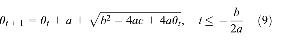
and

If

and

Equations (9)–(12) show that there exist two different cases for the approximate state equations, namely, equations (9) and (10) and equations (11) and (12). The case, which is more reasonable, accurate, and applicable, depends on the regressive coefficients (a, b, and c) and state parameter
The built BDNM
Based on section “The transformed state equation based on quadratic function,” the built BDNMs in this article are as follows:
The monitored equation is

If

and

If

and
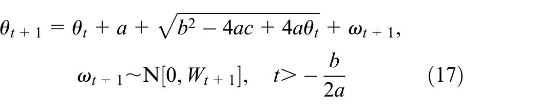
The initial state information

where a, b, and c are constants;
For BDNM,
With equations (13)–(18), the updating relationship between the monitored data and state parameters can be obtained as

It can be seen from equation (19) that the modeling processes of BDNM can be divided into two key steps. The first step is to obtain the priori probability distribution function (PDF) of
In this article, two methods are provided to deal with the built BDNM and the corresponding probability recursion processes. One method is to transform the built BDNM into BDLM with Taylor series expansion technique and the other one is directly to handle with the built BDNM and the probability recursion processes with MCMC simulation method.
Transformed BDLM and the corresponding probability recursion processes based on the built BDNM with Taylor series expansion technique
In this section, the Taylor series expansion technique is adopted to transfer the built BDNM into BDLM. Usually, quadratic function of the monitored extreme stress data can better fit the changing trend of the monitored data for long-term prediction, and the trend data mean the state data of the monitored data. The fitted quadratic function can be transformed into linear state equation with Taylor series expansion technique:
1. Linearization of nonlinear state equations
With Taylor series expansion technology, the nonlinear equations shown in equations (14)–(17) are transformed into approximate linear equation, namely

If a > 0, then
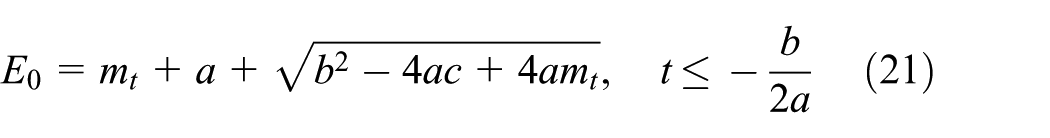
and


and

If a < 0, then

and


and
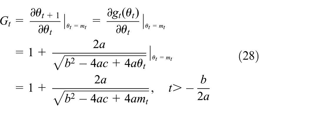
where
Furthermore, by combining equations (20)–(28), the transformed approximate linear state equation is

2. Transformed BDLM
The transformed BDLMs are as follows:
The monitored equation is approximately similar to equation (13).
The state equation

The initial information

3. The probability recursion processes of transformed BDLM
BDLMs are applicable to the prediction of the future state parameters. 14 With Bayesian method, the recursively updating processes of the transformed BDLM12,15 are as follows:
(a) The posteriori distribution at time t
For mean mt and variance matrix Ct, i = 1, 2, …, s, there is

(b) The priori distribution at time t + 1

where
(c) One-step prediction distribution at time t + 1

where
According to the definition of highest posterior density (HPD) region, 14 the predicted interval of the monitored data with a 95% confidential interval at time t + 1 is

where
(d) The posteriori distribution at time t + 1

where
The probability recursion processes based on the built BDNM with MCMC simulation method
The built BDNMs are shown in equations (13)–(18). With the monitored stress data, the probability function of the initial state parameters can be obtained with section “Determination of the main probability parameters of BDNM.” For example, the PDF of
Algorithm 1
With MCMC simulation method, draw a group of convergent sample
For every sample
For
Algorithm 2
For every sample
Let
Draw a sample
The same procedure is repeated M times, then let
Steps (1)–(4) are repeated N times; convergent sample
The distribution parameters of one-step prediction distribution are

where
In Algorithm 2, according to the Metropolis–Hastings (M-H) algorithm of MCMC simulation method,
Determination of the main probability parameters of BDNM
For the BDNM, the main probability parameters are Vt+1, Wt+1, mt, and Ct. The method of determining the main probability parameters is as follows.
In this article, the interval period of model updating is 1 day. Vt+1 is estimated with the variance of differences between the fitted trend data and monitored extreme stress data. According to the research,15,17,18Wt+1 can be solved with

where
If the initial state data follow the lognormal distribution, then the state data can be transformed into a quasi-normal distribution
17
with equations (40) and (41); the distribution parameters are, respectively,

where g( ) is the actual fitted PDF of the sample data (lognormal probability density function), and the actual PDF (lognormal PDF) is G( ) and G(x0) = 0.05.
Reliability prediction based on the built BDNM and FOSM
FOSM
In this article, the FOSM method19,20 is adopted to predict the reliability indices. Suppose there are random variables R (generalized resistance) and S (generalized load effects including dead load effects and live load effects) which are internally independent and mutually independent, the mean value and standard variance of which are, respectively, as follows:
The limit state function is

With FOSM method, the computation formula of the reliability indices can be obtained with

Reliability prediction formulas, respectively, based on the transformed BDLM and the built BDNM with FOSM method
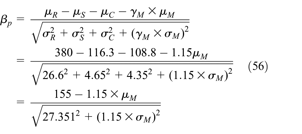
The limit state function of the second lateral span beam of some bridges is

where R is the steel yield strength, S is the stress caused by the dead weight of steel, C is the stress caused by the dead weight of the concrete, M is the monitored extreme stress predicted with the transformed BDLM or the built BDNM, and
Prediction formula of reliability indices based on the transformed BDLM with FOSM method
With FOSM method, based on equations (43) and (44) and the transformed BDLM, the predicted reliability index

where
Reliability prediction formula based on the built BDNM with FOSM method
With FOSM method, based on equations (43) and (44) and the built BDNM, the predicted reliability index
where
Application to an existing bridge
The I-39 Northbound Bridge, described in Frangopol and colleagues9,10 in detail, was built in 1961. It is a five-span continuous steel plate girder bridge. The total length of the bridge is 188.81 m. The explicit details about the aim and the results of the monitoring program for the whole bridge are given in Frangopol and colleagues.9,10 The extreme stress data at the beam bottom in the middle part of the second lateral span from the whole bridge are monitored for 83 days, and the corresponding limit state function is shown in equation (44). The monitored data displayed the variability of the stresses caused by traffic, temperature, shrinkage, creep, and structural changes. The stresses from the dead weight of the steel structure and the concrete deck are not included in the measured data. The day-by-day monitored extreme stress data are shown in Figures 2, 4, 6, and 7.
In this example, with equations (13)–(46), the trend data of the monitored data are directly fitted as

where
To obtain the distribution parameters of the initial state information, the monitored stress data of the 83 days are smoothly processed or resampled, and then the initial information (the resampled data) of the monitored data is approximately solved. Through Kolmogorov–Smirnov (K-S) test for the initial information, the initial priori PDF is the lognormal probability density distribution or normal probability density distribution as shown in Figure 1.

The initial priori probability density functions and the initial information.
BDNM based on the monitored data
With equations (13)–(18), the built BDNM is as follows.
The monitored equation is

The state equations are

and

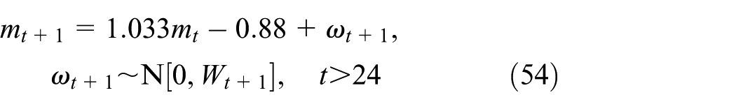
The initial state information

where yt+1 are the monitored extreme stress data at time t + 1. mt+1 is the state value of the monitored extreme stress at time t + 1.
Equation (51) shows that the initial information follows the normal distribution or lognormal distribution. So the following four cases are discussed to predict the monitored stress data:
Case 1. The initial state information follows the normal distribution, and then the BDNMs are built based on the normal distribution to predict the monitored extreme stresses with MCMC simulation method described in section “The probability recursion processes based on the built BDNM with MCMC simulation method.”
Case 2. The initial state information follows the lognormal distribution; first, the lognormal distribution must be transformed into a quasi-normal distribution, 17 and then the BDNMs are built based on the quasi-normal distribution to predict the monitored extreme stresses with MCMC simulation method described in section “The probability recursion processes based on the built BDNM with MCMC simulation method.”
Case 3. The arithmetic mean of the one-step prediction mean values, respectively, obtained with case 1 and case 2 is considered as the predicted extreme stresses of the third case.
Case 4. The fourth case is to build combinatorial BDNM with BDNM obtained with case 1 and case 2; the modeling processes of combinatorial BDNM are described in Jiang et al. 21 in detail.
From Figure 2, it is noticed that the predicted stress data of the four cases all fit the changing rules of the monitored extreme data, but as far as the prediction precisions of the four cases shown in Figure 3 are concerned, the combinatorial prediction precision is the best. So the combinatorial prediction model of the monitored stresses is adopted to predict the structural reliability indices.
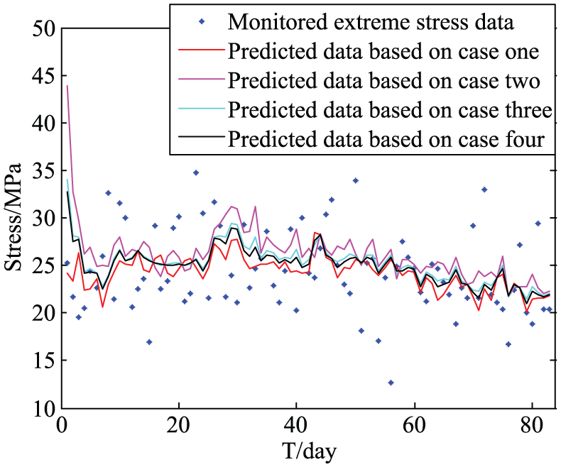
Monitored and predicted data based on the four cases of the built BDNM.

Prediction precision based on the four cases of the built BDNM.
BDLM based on the monitored data
Based on section “Transformed BDLM and the corresponding probability recursion processes based on the built BDNM with Taylor series expansion technique” and equations (48)–(51), the built approximate BDLMs are as follows:
The monitored equation

The transformed approximately linear state equation

and
The initial state information

where
Equation (55) shows that the initial state information follows the normal distribution or lognormal distribution. So the following four cases are discussed to predict the monitored extreme stresses:
Case 1. The initial state information follows the normal distribution, and then the transformed BDLMs are built based on the normal distribution to predict the stress data.
Case 2. The initial state information follows the lognormal distribution; first, the lognormal distribution must be transformed into a quasi-normal distribution,17,18 and then the BDLM is built based on the quasi-normal distribution to predict the stress data.
Case 3. The arithmetic mean of the one-step prediction mean values, respectively, obtained with case 1 and case 2 is considered as the predicted extreme stresses of the third case.
Case 4. The fourth case is to build combinatorial BDLM with BDLM obtained with case 1 and case 2; the modeling processes of combinatorial BDLM are described in Jiang et al. 21 and Liu et al. 22
From Figure 4, it is noticed that the predicted stress data of the four cases all fit the changing rules of the monitored stress data, but as far as the prediction precisions of the four cases shown in Figure 5 are concerned, the combinatorial prediction precision is the best. So the combinatorial prediction model (case 4) of the monitored extreme stress is adopted to predict the structural reliability indices.

Predicted extreme stresses based on the four cases of the transformed BDLM.

Prediction precision based on the four cases of the transformed BDLM.
Reliability prediction based on the BDNM (case 4) and transformed BDLM (case 4)
In Figures 3 and 5, we can know that the combinatorial prediction model is the best. So the combinatorial prediction model of the stresses is adopted to predict the structural reliability indices. The predicted results, which are shown in Figures 6–8, can show the changing trends and the ranges of the monitored reliability indices. The design specifications are as follows. 9
assigned to the bottom of the girder in the middle of the second lateral span which is shown in Frangopol and colleagues,9,10 where

Reliability indices based on case 4 of BDNM.

Reliability indices based on case 4 of the transformed BDLM.

Comparison of reliability indices obtained with the built BDNM (case 4) and the transformed BDLM (case 4).
Conclusion
The article first builds the BDNM based on the quadratic function and the monitored data, and then two methods are proposed to handle with the probability recursion processes; finally, based on the predicted stress data, the structural reliability indices are predicted with FOSM method. The following conclusions can be reached: from the prediction results shown in Figures 2–8, the prediction value and predicted range of the stress and reliability indices all fit the changing rules of the corresponding performances with the proposed two methods in this article, and the prediction precisions are both better and better with the updating of the monitored data.
Footnotes
Acknowledgements
The authors would like to thank the editor and the anonymous reviewers for their constructive comments and valuable suggestions to improve the quality of the article.
Academic Editor: Jun Li
Declaration of conflicting interests
The author(s) declared no potential conflicts of interest with respect to the research, authorship, and/or publication of this article.
Funding
The author(s) disclosed receipt of the following financial support for the research, authorship, and/or publication of this article: This work was supported by the National Natural Science Foundation of China (project no. 51608243), the Natural Science Foundation of Gansu Province of China (project no. 1606RJYA246), and the Fundamental Research Funds for the Central Universities (lzujbky-2015-300, lzujbky-2015-301).