Analysis of thermal deformation and influencing factors in shrink-fitting assembly of aluminum alloy drill pipe

Abstract

In shrink-fitting assembly process of aluminum alloy drill pipe with steel joint, the relationship between cooling water velocity, initial heating temperature, and thermal deformation of the steel joint is an important factor to ensure the long-term reliability of the connection and the performance. In this article, the shrink-fitting assembly experiment of aluminum pipe with steel joint was conducted and the accurate experimental data were obtained for temperature field. A finite element method was then applied to simulate the temperature field of steel joint and compared with the experimental results. Based on the thermo-elasticity theories, an analytical solution was developed to calculate the thermal deformation in radial direction within the same cross section. A least-square fitting procedure was used to determine the thermal deformation of steel joint. A relationship diagram among these three factors was established, which is particularly important in predicting the minimum heating temperature of steel joint and the minimum cooling water velocity. Based on the above analysis, a method to select the initial heating temperature and the cooling water velocity was provided and the optimum values of the magnitude of interference, the initial heating temperature, and the cooling water velocity were obtained.

Introduction

With the rapid development of oil and gas industry together with advances in the geological exploration industry, drilling depth has also been greatly increasing, this exerting higher requirements on working properties of drilling pipes. Compared to steel drill pipes, aluminum alloy drill pipes are more advantageous in well drilling because of low specific gravity, corrosion resistance under various harsh environments, non-magnetic property, and stable mechanical properties. For drilling rigs of the same hook load capacity, aluminum alloy drill pipes allow for significantly reduced power consumption and time of drilling operations, as well as increased drilling capacity, compared to ordinary steel drill pipes. Aluminum alloy pipe bodies are usually assembled with regular steel joints to form drill strings.

MI Lourenco et al. ¹ conducted extensive research on the structural strength of aluminum alloy drill pipes, with the aim to improve the fatigue resistance of these components by selecting the appropriate aluminum alloys and strengthening the threaded connection of steel joints. GF Miscow et al.^2,3 introduced experimental testing procedures targeting different pipe materials (Al–Zn–Mg alloys) and sizes and performed numerical analysis.

During assembly, the steel joint is heated and then screwed to the end of the aluminum alloy pipe; after cooling, the assembly can provide a reliable permanent connection. V Tikhonov et al. studied the stress distribution within the assembly in detail and calculated the stress concentration factors under different axial loads, flexural moment ranges, interference friction coefficients, and interference magnitudes of connection. Furthermore, they conducted fatigue testing on full-size aluminum alloy pipe connections using four-point bending fatigue machine and resonant fatigue test machine and comparatively verified the findings with simulation analysis results. ⁴

V Tikhonov et al. proposed a fixed torque method and a heat assembly method for connection of aluminum alloy drill pipes with steel joints. In the first method, the male and female steel joints are tightened on the aluminum alloy drill pipe with sufficiently high torque; while in the second method, steel joint is heated and then screwed to the end of aluminum alloy pipe, and after cooling, the joint contracts to form a reliable permanent threaded connection of “aluminum alloy drill pipe-steel joint.” In this article, an analysis is pursued regarding intensities of tensile loads and alternating bending loads borne by these two types of connections after assembly. Subsequently, tensile test is performed on full-size aluminum alloy drill pipes on Krylov Shipbuilding’s MUG-3000 load test machine to analyze the results of the two assembly methods. ⁵ J Mao et al. ⁶ studied the interference connection of aluminum alloy drill pipe body–steel tool joint assembly and both assembling technique and the temperature are introduced.

As the finite element technology develops, finite element method is used for studying heat transfer and thermal deformation problems of mechanical parts.^7–11 Pelosi and Ivantysynova ¹² conducted study of temperature field distribution and thermal deformation on piston and contact surface of piston cylinder with finite element method. XW Yang et al. ¹³ conducted a study on temperature field and stress field of aluminum alloy and other large-scale complicated thin-walled members during the process of quenching with finite element simulation method.

As the science and technology constantly develops in recent years, the demand for accurate calculation and measurement of the thermal deformation of mechanical parts is increasing. A significant amount of practical engineering problems force people to seek out perfection of the thermal expansion mechanism; thus, the classic thermal expansion theory never stops to develop. Hu Penghao and Li Guihua proposed the theory model of non-uniform temperature field of parts in different conditions based on the theories of thermal conduction, elasticity, and thermal elasticity. They carried out a systematic theoretical analysis and experimental verification for thermal deformation and thermal stress of parts. Meanwhile, they conducted systematic theoretical analysis and substantial experimental work on thermal deformation and relevant contents of mechanical parts with complicated surface based on the study of simple geometric parts.^14–16 The thermal elasticity theory finds numerous applications for solving thermal deformation problems of various new-type materials and complicated mechanical parts. H Yaghoobi and A Fereidoon ¹⁷ proposed an improved n-order shearing deformation theory aiming at functionally graded materials on the basis of thermo-elasticity mechanics. HK Yi et al. ¹⁸ established a thermal deformation analysis model of carbon steel double-layered tube pursuant to the equilibrium equation of thermo-elasticity mechanics and conducted a study on circumferential thermal stress and crack thermal deformation. The thermal deformation theory is also widely used in the thermal deformation study of key parts such as machine tool and principal axis.^19,20 J Vyroubal ²¹ conducted thermal deformation amount measurement for the stand column and principal axis of machine tool with the decomposition method and studied on the thermal deformation compensation of principal axis of machine tool.

In this article, connection between aluminum alloy pipe bodies and steel joints is pursued on the basis of the interference fitting-based heat assembly technique. The study of flow rate of cooling water, initial heating temperature, and thermal deformation amount of the joint during shrink-fitting assembly process is of great importance. Therefore, getting the relationship among these three factors is of great significance on the basis of studying temperature field and thermal deformation of steel joint. The first part of this article introduced the experimental process of the shrink-fitting assembly and the arrangement of the measured points. The second part first analyzed the measurement results of temperature field, presented the finite element simulation of temperature field, and contrastively analyzed the simulation and experiment results. The third party used thermal deformation analytical method of steel joint to establish the equation of temperature function with least-square method. The calculation results of thermal deformation were got and analyzed. The fourth party studied the selection for magnitude of interference and influencing factors. Conclusions of this study are presented at the end.

Introduction to shrink-fitting assembly experiment

The abrasive resistance of aluminum alloy drill pipe was relatively lower; thus, it could not be twisted and disassembled frequently during drilling process. Therefore, it was needed to assemble the pipe body of the aluminum alloy drill pipe with steel joint to form the drill column, thus making the steel joint twisted and disassembled. Shrink-fitting assembly technology was used to connect the pipe body of the aluminum alloy drill pipe and steel joint to achieve a reliable connection. The well-known shrink-fitting assembly referred to heating the steel joint to a certain temperature, making it expand, and twisting it on aluminum alloy pipe in heat condition. Gain necessary pre-tightening force in the position of screw connection, get fixed permanent connection, and achieve the aim of reliable connection by interference fit.

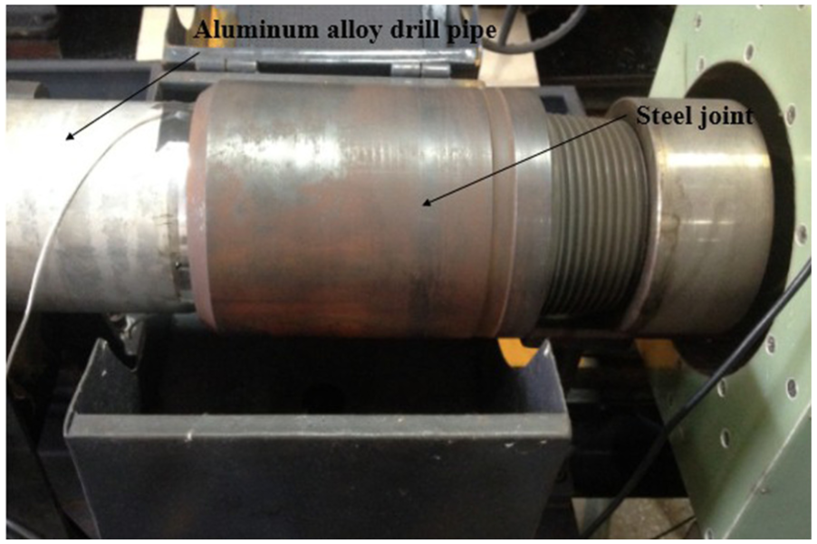
The aluminum alloy drill pipe was fixed as shown in Figure 1. An induction heater was used to heat the steel joint to required temperature. After heating, the steel joint rapidly moved toward left, making the internal thread of steel joint contact with the pipe body of aluminum alloy drill pipe. Meanwhile, the steel joint started to rapidly rotate back and screwed in pipe body of aluminum alloy drill pipe along the threads. Finally, shrink-fitting assembly process was completed as shown in Figure 2.

Figure 1.

Schematic illustration of shrink-fitting assembly starting.

Figure 2.

Schematic illustration of screwing completion.

In order to prevent high temperature for the aluminum alloy drill pipe due to contacting with high-temperature steel joint and avoid reduction in the mechanical property of aluminum alloy materials, a cooling device inside pipe body of aluminum alloy drill pipe should be kept open during the whole process of shrink-fitting assembly so as to cool the interior of aluminum alloy drill pipe, guaranteeing the temperature of external thread of drill pipe. Closed circulation of internal cooling water is shown in Figure 1. The cross-sectional area of cooling water is constant in the heat transfer area between the inner wall of the pipe and the cooling water, so the cooling water velocity is constant. The cooling water velocity v is the water velocity through any cross-sectional area in drill pipe, as shown in Figure 1.

The main study aims of this article were to explore the relationship among cooling water rate, initial heating temperature, and thermal deformation amount of the steel joint.

Therefore, the measurement of temperature at B and C is shown in Figure 3. Shrink-fitting assembly experiment and temperature measurement were all conducted on the shrink-fitting assembly experimental platform of aluminum alloy drill pipe, shown in Figure 4.

Figure 3.

Measurement point position of steel joint.

Figure 4.

Experimental device of shrink-fitting assembly.

Experiment and temperature field simulation of shrink-fitting assembly

Experimental results and analysis

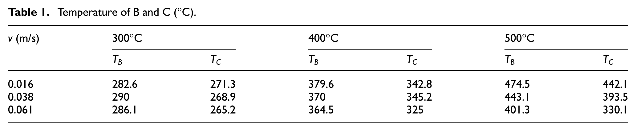
The experimental temperature was 22°C, and the initial temperature of cooling water was guaranteed at 20°C. The process from the contact of steel joint with aluminum alloy drill pipe to completely tightening needed 30 s. This assembly time was kept unchanged. Experiments were conducted under the condition that the steel joint was separately heated to 300°C, 400°C, and 500°C and the cooling water velocity was 0.016, 0.038, and 0.061 m/s, respectively; there are 3 × 3 = 9 group experiments. According to the experiment, temperature values at points B and C of the steel joint with different cooling water velocity, when the steel joint was completely tightened, are shown in Table 1 and can be further found in Figures 5 and 6.

Table 1.

Temperature of B and C (°C).

v (m/s)	300°C		400°C		500°C
	$T_B$	$T_C$	$T_B$	$T_C$	$T_B$	$T_C$
0.016	282.6	271.3	379.6	342.8	474.5	442.1
0.038	290	268.9	370	345.2	443.1	393.5
0.061	286.1	265.2	364.5	325	401.3	330.1

Figure 5.

Temperature of B when 30 s.

Figure 6.

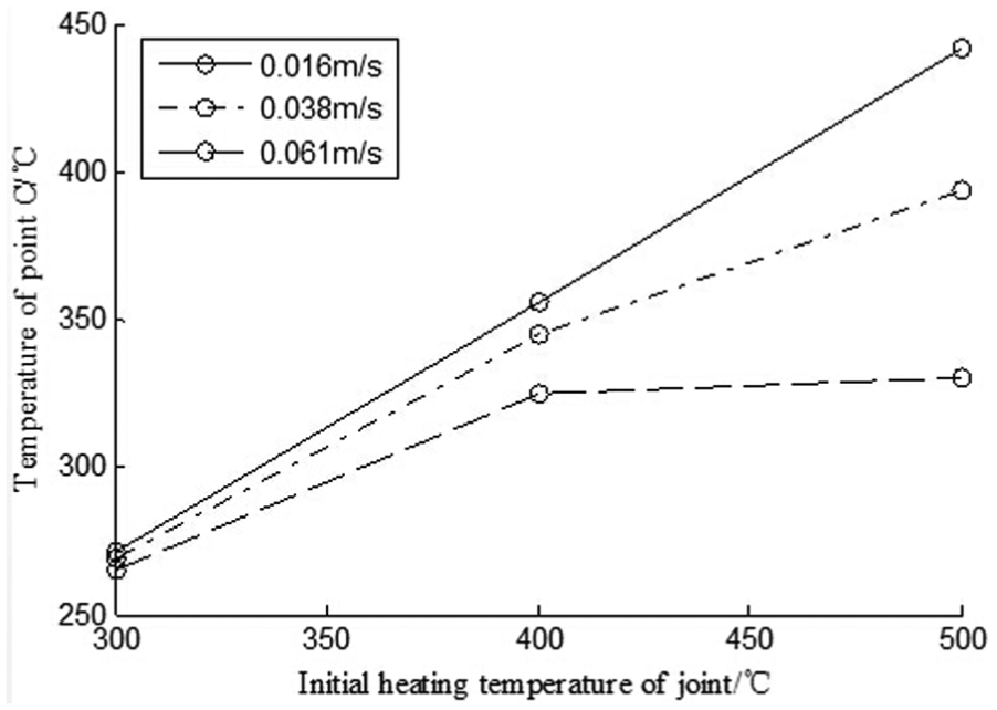
Temperature of C when 30 s.

According to Figure 5, it can be seen that the temperature of point B constantly increased when the heating temperature of steel joint increased with different cooling water velocity. By observing the three curves, it can be seen that the temperature at point B had little differences for 0.016 and 0.061 m/s at 300°C. However, with the increase in initial temperature of steel joint, the curve slope at 0.016 m/s was significantly larger than that of 0.061 m/s. In other words, with the reduction in flow rate of cooling water, the increase in initial temperature of steel joint would cause a rapid increase in the temperature at point B when tightening. According to Figure 6, a similar conclusion could be drawn for point C, results in this case being more apparent. Thus, it could be noted that the higher the initial heating temperature of steel joint, the more apparent effects of cooling water velocity exerting on the temperature change of steel joint.

Table 2 and Figure 7 could be obtained from Table 1. From an analysis of data in Figure 7, it can be seen that with the increase in initial heating temperature of the steel joint and under the same cooling water velocity, the temperature difference between B and C constantly increased. For the same initial heating temperature of joint, temperature difference between B and C constantly increased with the increase in cooling water velocity. This indicated that increasing the heating temperature of joint or increasing the flow rate of cooling water could increase the cooling heterogeneity of cooling water in axis direction.

Table 2.

Temperature difference between B and C (°C).

v (m/s)	300°C	400°C	500°C
	$\Delta T=T_B-T_C$	$\Delta T=T_B-T_C$	$\Delta T=T_B-T_C$
0.016	18.8	23.8	32.4
0.038	20.2	28	49.6
0.061	20.9	39.5	71.2

Figure 7.

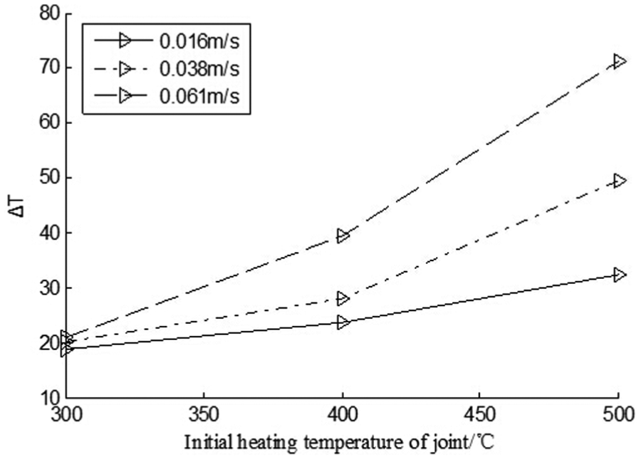
Temperature difference (°C) between B and C when 30 s.

Taking the cooling water velocity as y coordinate, initial heating temperature of joint as x coordinate, and measurement point temperature of steel joints as z coordinate, the temperature of three-dimensional (3D) surface chart of B and C was derived, as shown in Figures 8 and 9. According to these figures, the temperature value of B and C could be easily confirmed when completing the screwing operation of threads under any cooling water velocity and any initial heating temperatures of joints in certain scope, laying the foundation for further calculating expansion amount.

Figure 8.

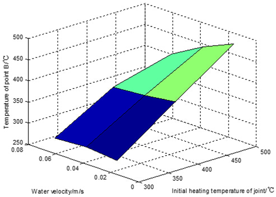
Temperature relationship figure of B when 30 s.

Figure 9.

Temperature relationship figure of C when 30 s.

Finite element simulation of shrink-fitting assembly temperature field

The construction of the 3D geometry model is the basis for the finite element analysis. A geometric model in accordance with the actual size of steel joint and aluminum alloy drill pipe is established. In the assembly process, heat from steel joints flows into aluminum alloy drill pipe mainly along the normal of thread contact surface. So, under the assumption that they are in close contact, the contact surface of aluminum alloy drill pipe and steel joint can be reasonably approximated as a conical surface. The heat flux inside the drill pipe concentrates on the contact part of the cooling water and the drill pipe’s inner wall, and the cooling water flows along the axial direction, so the internal cooling system can be simplified as boundary of heat convection. The boundary between the system and the air is set to natural convection heat transfer boundary as shown in Figure 10.

Figure 10.

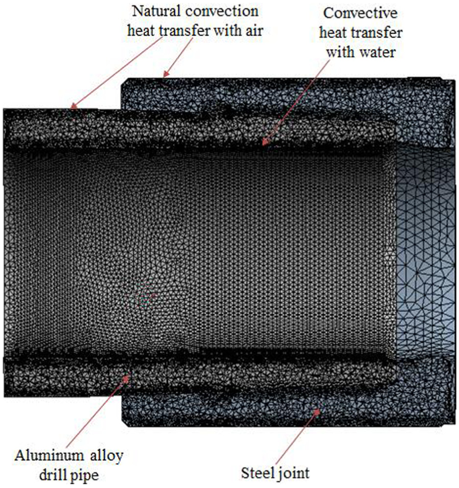
Finite element mesh generation and boundary setting.

The domain is meshed using tetrahedron elements. The mesh size is 1 mm, and the mesh size of the contact surface is refined as 0.5 mm. The element number is 3,692,564 and the node number is 5,118,747, as shown in Figure 10.

We set ambient temperature as 22°C, cooling water temperature as 20°C, initial temperature of aluminum alloy drill pipe as 20°C, simulation time as 30 s, the initial heating temperature as 300°C/400°C/500°C, and set the flow rate of cooling water as 0.016, 0.038, and 0.061 m/s.

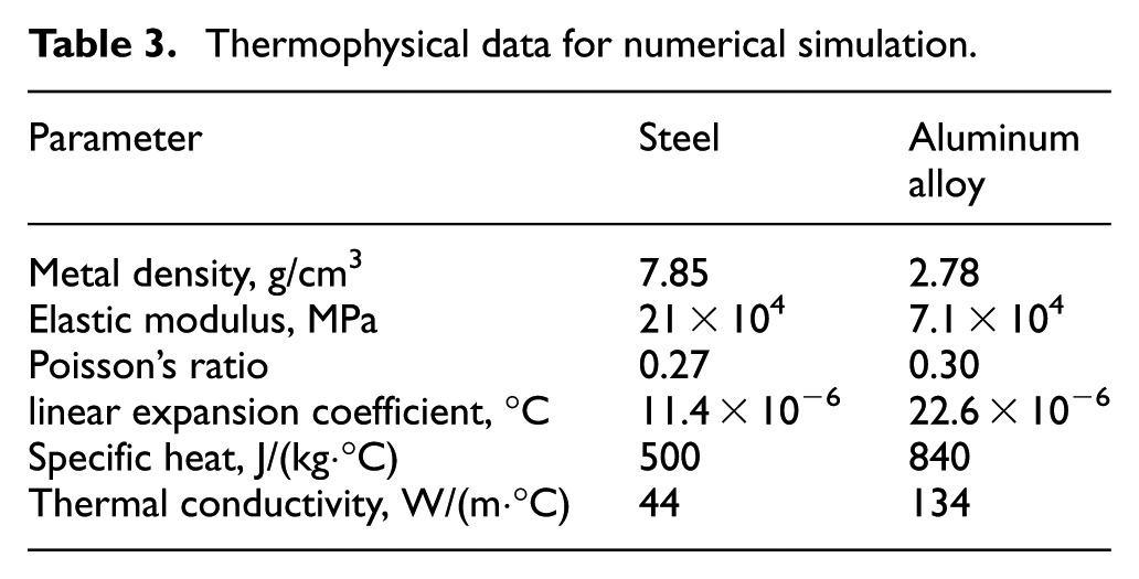
The thermophysical data for the aluminum alloy drill pipe and the steel joint used in the simulation are listed in Table 3. The convective heat transfer coefficients h between the internal wall of the aluminum alloy pipe and the cooling water, under different flow rates of cooling water, are set as shown in Table 4. The natural convection heat transfer coefficient is set as $1\times {10}^{-5}\mathrm{W}/(\mathrm{m}{\mathrm{m}}^2·°\mathrm{C})$ .

Table 3.

Thermophysical data for numerical simulation.

Parameter	Steel	Aluminum alloy
Metal density, g/cm3	7.85	2.78
Elastic modulus, MPa	21 × 104	7.1 × 104
Poisson’s ratio	0.27	0.30
linear expansion coefficient, °C	11.4 × 10−6	22.6 × 10−6
Specific heat, J/(kg·°C)	500	840
Thermal conductivity, W/(m·°C)	44	134

Table 4.

Convective heat transfer coefficients.

Q, L/min	20	15	10	5
h, W/(m2·K)	760	560	430	310

Analysis on temperature field experiment and simulation results

According to the finite element model of the previous section, we set ambient temperature as 22 °C, cooling water temperature as 20 °C, initial temperature of aluminum alloy drill pipe as 20 °C, simulation time as 32 s, heat the steel joints to 300°C/400°C/500°C, and set the flow rate of cooling water as 0.016, 0.038, and 0.061 m/s to carry out the simulation in order to obtain the temperature distributions of steel joints at the time point of 30 s, under different flow rates of cooling water and initial heating temperatures. Due to space limitations, we listed only the temperature profiles of steel joints under the flow rate 0.016 m/s, as shown in Figures 11–13.

Figure 11.

Temperature distribution of screwed joints under 0.038 m/s and heated to 300°C.

Figure 12.

Temperature distribution of screwed joints under 0.038 m/s and heated to 400°C.

Figure 13.

Temperature distribution of screwed joints under 0.038 m/s and heated to 500°C.

Figures 11–13 show that the temperatures of joints were higher at point B and decreased gradually along the axis toward point C. Thus, among the threaded portion, temperature had the highest value at point B and the lowest value at point C, this indicating that it is reasonable to set sensors at points B and C. The temperature of the entire joint decreased gradually from outer surface to inner surface. The simulation results of temperature field distributions of the joints provided the necessary conditions for further calculations on thermal deformation.

Based on the above simulation results, we obtained the simulated and experimental values for the highest temperature of threads under different flow rates of cooling water. The comparison between simulated values $T_S$ and experimental values $T_E$ for the highest temperature of threads is shown in Table 5. It can be seen that $|T_E-T_S|\le$ 2.4 was suitable for various flow rates and joint temperatures, thereby the reasonableness of simulation results was verified.

Table 5.

Comparison of experimental value and simulation value for temperatures at points B and C (°C).

v (m/s)		300°C		400°C		500°C
		$T_B$	$T_C$	$T_B$	$T_C$	$T_B$	$T_C$
0.016	$T_E$	290.1	271.3	379.6	355.8	474.5	442.1
	$T_S$	290.2	270.8	380.8	356.6	476.0	443.6
	$|T_E-T_S|$	0.1	0.5	1.2	0.8	1.5	1.5
0.038	$T_E$	289.1	268.9	373.2	345.2	443.1	393.5
	$T_S$	288.3	268.1	374.1	345.1	445.5	394.9
	$|T_E-T_S|$	0.8	0.8	0.9	0.1	2.4	1.4
0.061	$T_E$	286.1	265.2	364.5	325	401.3	330.1
	$T_S$	286.6	265.7	365.1	325.1	402.6	330.7
	$|T_E-T_S|$	0.5	0.5	0.6	0.1	1.3	0.6

Study on thermal deformation of steel joints

Relationship among initial heating temperature of joint, flow rate of cooling water, and joint deformation was an important process parameter for shrink-fitting assembly. After the temperature simulation, we need to discuss the hot deformation process of steel joint based on its temperature field results. Therefore, in this article, we studied on deformation of the joint using the thermal elasticity theory.

Thermo-elasticity was extended from the elasticity. According to general material mechanics, it was appreciated that the root cause for stress was the load. However, in fact, the deformation could be caused by the load, as well as the temperature changes. If an object’s temperature was changing and it could not be deformed freely due to externally or internally constraints, then the temperature-changing stress would occur. The root cause for thermal stress was the force generated during temperature changing without any external force. Thermal stress involved mainly the analysis on relationship between physical properties and temperatures of the object; in addition, it also involved the knowledge about thermodynamics and heat transfer. On the basis of certain equations, we only needed the temperature field function to obtain the expressions for stress, strain, and displacement in an attempt to simplify the problems to be solved.

Analysis method for thermal deformation of steel joints

Since the joint was axial symmetric, we considered that the joint was composed of several rings with thickness $\delta$ as shown below. If $\delta$ was small enough, we could ignore the influence from the taper of inner surface of the joint on the inner diameter a of the ring within the thickness; moreover, the ring could be seen as a plane stress-related problem, namely, ${\sigma }_z=0$ ; since the temperature profile was axisymmetric and the temperature T was a function of the radius r, the radial displacement $u_r$ depended only on the radius r.

For those thin rings with same thickness shown in Figure 14, the distributions of stress and strain were axial symmetric as well. Using polar coordinate analysis, we considered this problem belonged to a plane stress-related problem, whose balance equation is as follows

$$\{\begin{array}{c}\frac{\partial {\sigma }_r}{\partial r}+\frac{1}{r}\frac{\partial {\tau }_{r\theta }}{\partial \theta }+\frac{{\sigma }_r-{\sigma }_{\theta }}{r}=0\hfill \\ \multicolumn{1}{c}{\frac{1}{r}\frac{\partial {\sigma }_{\theta }}{\partial \theta }+\frac{\partial {\tau }_{r\theta }}{\partial r}+\frac{2{\tau }_{r\theta }}{r}=0}\end{array}$$

(1)

where ${\sigma }_r$ is the radial normal stress, ${\sigma }_{\theta }$ is the radian normal stress, and ${\tau }_{r\theta }$ is the shear stress.

Figure 14.

Schematic diagram of the ring.

As being an axisymmetric problem, the balance equation could be

$$\{\begin{array}{c}\frac{\partial {\sigma }_r}{\partial r}+\frac{{\sigma }_r-{\sigma }_{\theta }}{r}=0\hfill \\ \multicolumn{1}{c}{\frac{\partial {\sigma }_{\theta }}{\partial \theta }=0}\end{array}$$

(2)

Simplified geometric equation is as follows

$$\{\begin{array}{c}{\epsilon }_r=\frac{\partial u_r}{\partial r}\hfill \\ \multicolumn{1}{c}{{\epsilon }_{\theta }=\frac{u_r}{r}}\end{array}$$

(3)

Physical equation is as follows

$$\{\begin{array}{c}{\epsilon }_r=\frac{1}{E}({\sigma }_r-\mu {\sigma }_{\theta })+\alpha T\hfill \\ \multicolumn{1}{c}{{\epsilon }_{\theta }=\frac{1}{E}({\sigma }_{\theta }-\mu {\sigma }_r)+\alpha T}\end{array}$$

(4)

where E is the elastic modulus of the material, $\mu$ is Poisson’s ratio of the material, and $\alpha$ is the linear expansion coefficient of the material.

Let the stress be represented by the strain

$$\{\begin{array}{c}{\sigma }_r=\frac{E}{1-{\mu }^2}({\epsilon }_r+\mu {\epsilon }_{\theta })-\frac{E\alpha T}{1-\mu }\hfill \\ \multicolumn{1}{c}{{\sigma }_{\theta }=\frac{E}{1-{\mu }^2}({\epsilon }_{\theta }+\mu {\epsilon }_r)-\frac{E\alpha T}{1-\mu }}\end{array}$$

(5)

Substitute formula (3) into formula (5)

$$\{\begin{array}{c}{\sigma }_r=\frac{E}{1-{\mu }^2}(\frac{d{u}_r}{\mathrm{dr}}+\mu \frac{u_r}{r})-\frac{E\alpha T}{1-\mu }\hfill \\ \multicolumn{1}{c}{{\sigma }_{\theta }=\frac{E}{1-{\mu }^2}(\frac{u_r}{r}+\mu \frac{d{u}_r}{\mathrm{dr}})-\frac{E\alpha T}{1-\mu }}\end{array}$$

(6)

Subtract for formula (6)

$${\sigma }_r-{\sigma }_{\theta }=\frac{E}{1+\mu }({\epsilon }_r-{\epsilon }_{\theta })$$

(7)

Solve the derivative of r for equation (7) and substitute the geometric equation (3) into equation (7)

$${\sigma }_r-{\sigma }_{\theta }=\frac{E}{1+\mu }({\epsilon }_r-{\epsilon }_{\theta })=\frac{E}{1+\mu }(\frac{d{u}_r}{\mathrm{dr}}-\frac{u_r}{r})$$

(8)

Solve the derivative of r for equation (8) and substitute the geometric equation (3) into equation (8)

$$\begin{array}{c}\multicolumn{1}{c}{\frac{\partial {\sigma }_r}{\partial r}=\frac{E}{1-{\mu }^2}({\epsilon \prime }_r+\mu {\epsilon \prime }_{\theta })-\frac{E\alpha }{1-\mu }·\frac{\mathrm{dT}}{\mathrm{dr}}}\\ \multicolumn{1}{c}{=\frac{E}{1-{\mu }^2}[\frac{d}{\mathrm{dr}}\left(\frac{d{u}_r}{\mathrm{dr}}\right)+\mu \frac{d}{\mathrm{dr}}\left(\frac{u_r}{r}\right)]-\frac{E\alpha }{1-\mu }·\frac{\mathrm{dT}}{\mathrm{dr}}}\\ \multicolumn{1}{c}{=\frac{E}{1-{\mu }^2}[\frac{d^2{u}_r}{d{r}^2}+\mu (\frac{{u\prime }_r}{r}-\frac{u_r}{r^2})]-\frac{E\alpha }{1-\mu }·\frac{\mathrm{dT}}{\mathrm{dr}}}\end{array}$$

(9)

If we substitute formulas (8) and (9) into formula (2), we get

$$\frac{E}{1-{\mu }^2}\left[\frac{d^2{u}_r}{d{r}^2}+\mu \left(\frac{{u^{\prime }}_r}{r}-\frac{u_r}{r^2}\right)\right]-\frac{E\alpha }{1-\mu }·\frac{dT}{dr}+\frac{E}{1+\mu }\left(\frac{d{u}_r}{dr}-\frac{u_r}{r}\right)=0$$

(10)

If the equation was multiplied by $(1-{\mu }^2)/E$ on both sides simultaneously, there would be

$$\begin{array}{c}\multicolumn{1}{c}{\alpha (1+\mu )\frac{\mathrm{dT}}{\mathrm{dr}}=\frac{d^2{u}_r}{d{r}^2}+\frac{1}{r}\frac{d{u}_r}{\mathrm{dr}}+\frac{1}{r^2}{u}_r}\\ \multicolumn{1}{c}{=\frac{d}{\mathrm{dr}}\left[\frac{1}{r}\frac{d(r·u_r)}{\mathrm{dr}}\right]}\end{array}$$

(11)

Integrating both sides of the equation, we obtain

$$\frac{d(r·u_r)}{\mathrm{dr}}=r\alpha (1+\mu )T+\mathrm{rC}$$

(12)

Integrating both sides of the equation again, we get

$$r·u_r=\alpha (1+\mu )\underset{a}{\overset{r}{\int }}\mathrm{Trdr}+C_1{r}^2+C_2$$

(13)

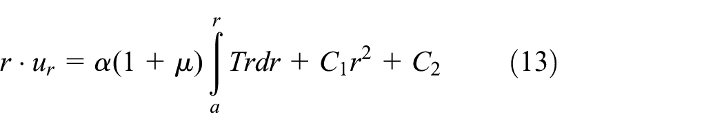
If both sides of the equation were multiplied by $1/r$ , there would be the thermal displacement function of disk parts as follows

$$u_r=\frac{\alpha (1+\mu )}{r}{\displaystyle \underset{a}{\overset{r}{\int }}Trdr+C_{1}r+\frac{C_2}{r}}$$

(14)

Get the derivative of r for formula (14), we obtain

$$\frac{d{u}_r}{\mathrm{dr}}=\alpha (1+\mu )(T-\frac{1}{r^2}\underset{a}{\overset{r}{\int }}\mathrm{Trdr})+C_1-\frac{C_2}{r^2}$$

(15)

If formula (14) was multiplied by $1/r$ , we get

$$\frac{u_r}{r}=\frac{\alpha (1+\mu )}{r^2}\underset{a}{\overset{r}{\int }}\mathrm{Trdr}+C_1+\frac{C_2}{r^2}$$

(16)

If formulas (15) and (16) were substituted into the ${\sigma }_r$ of formula (6), there would be the radial stress as follows

$$\begin{array}{c}\multicolumn{1}{c}{{\sigma }_r=\frac{E}{1-{\mu }^2}[\alpha (1+\mu )(T-\frac{1}{r^2}\underset{a}{\overset{r}{\int }}\mathrm{Trdr})+C_1-\frac{C_2}{r^2}}\\ \multicolumn{1}{c}{+\frac{\mu \alpha (1+\mu )}{r^2}\underset{a}{\overset{r}{\int }}\mathrm{Trdr}+\mu C_1+\frac{\mu C_2}{r^2}]-\frac{E\alpha T}{1-\mu }}\\ \multicolumn{1}{c}{=\frac{E}{1-{\mu }^2}[\alpha (1+\mu )T-\frac{\alpha (1-{\mu }^2)}{r^2}\underset{a}{\overset{r}{\int }}\mathrm{Trdr}}\\ \multicolumn{1}{c}{+(1+\mu )C_1-\frac{(1-\mu )C_2}{r^2}]-\frac{E\alpha T}{1-\mu }}\\ \multicolumn{1}{c}{=\frac{E\alpha T}{1-\mu }-\frac{E\alpha }{r^2}\underset{a}{\overset{r}{\int }}\mathrm{Trdr}+\frac{E{C}_1}{1-\mu }-\frac{E{C}_2}{r^2(1+\mu )}-\frac{E\alpha T}{1-\mu }}\\ \multicolumn{1}{c}{=-\frac{E\alpha }{r^2}\underset{a}{\overset{r}{\int }}\mathrm{Trdr}+\frac{E{C}_1}{1-\mu }-\frac{E{C}_2}{r^2(1+\mu )}}\end{array}$$

(17)

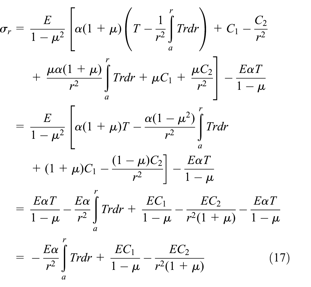
According to the boundary conditions ${{\sigma }_r|}_{r=a}=0$ and ${{\sigma }_r|}_{r=b}=0$ , the equations containing integration constants $C_1$ and $C_2$ could be determined as follows

$$\{\begin{array}{c}\frac{E{C}_1}{1-\mu }-\frac{E{C}_2}{a^2(1+\mu )}=0\hfill \\ \multicolumn{1}{c}{-\frac{E\alpha }{r^2}\underset{a}{\overset{b}{\int }}\mathrm{Trdr}+\frac{E{C}_1}{1-\mu }-\frac{E{C}_2}{b^2(1+\mu )}=0}\end{array}$$

(18)

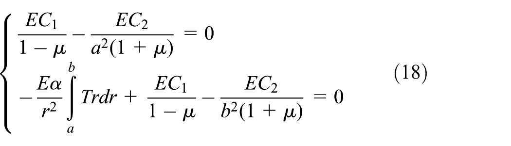
Solving the above equations, we obtain

$$\{\begin{array}{c}{C}_1=\frac{(1-\mu )\alpha }{b^2-a^2}\underset{a}{\overset{b}{\int }}\mathrm{Trdr}\hfill \\ \multicolumn{1}{c}{C_2=(1+\mu )\frac{\alpha ·a^2}{b^2-a^2}\underset{a}{\overset{b}{\int }}\mathrm{Trdr}}\end{array}$$

(19)

If $C_1$ and $C_2$ were substituted into formula (14), there would be radius-directional thermal deformation for any points on the disk as follows

$$u_r=\frac{\alpha }{r}[(1+\mu )\underset{a}{\overset{r}{\int }}\mathrm{Trdr}+\frac{(1-\mu )r^2+(1+\mu )a^2}{b^2-a^2}\underset{a}{\overset{b}{\int }}\mathrm{Trdr}]$$

(20)

Establishment of function relationship between temperature T and radius r

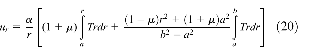
Based on the analysis method for thermal deformation in the previous section, we conducted radial thermal deformation calculations for cross section of the joints. The analysis in the previous section showed that the temperature T was a function of radius r; therefore, we needed to find the function relationship between T and radius r.

According to the simulation results in section “Analysis on temperature field experiment and simulation results,” we knew that the joints’ temperatures were changing uniformly from inside to outside; therefore, we considered that there was a simple linear relationship between T and r. Therefore, in this article, we used the linear equation of the least-square fitting function T(r).

If the fitting linear equation was to be solved as follows

$$T=c+d·r$$

(21)

where c and d are the regression coefficients.

Considering the deviations, the regression model would be

$$T=c+d·r+\epsilon$$

(22)

where $\epsilon$ is the deviation.

The corresponding least-square constraint criteria would be

$$Q=\sum _{i=1}^n{\epsilon }_i^2=\sum _{i=1}^n{(T_i-c-d{r}_i)}^2=min$$

(23)

where Q is the sum of squared deviations and ${\epsilon }_i$ is the deviation of the ith sample point.

If partial derivative of c from Q is equal to 0 and partial derivative of d from Q is equal to 0, there would be the minimum value

$$\{\begin{array}{c}\frac{\partial Q}{\partial c}=2\sum _{i=1}^n(T_i-c-d{r}_i)=0\hfill \\ \multicolumn{1}{c}{\frac{\partial Q}{\partial d}=2\sum _{i=1}^n(T_i-c-d{r}_i)r_i=0}\end{array}$$

(24)

Furthermore, there would be

$$\{\begin{array}{c}\sum _{i=1}^n{T}_i-\mathrm{nc}-d\sum _{i=1}^n{r}_i=0\hfill \\ \multicolumn{1}{c}{\sum _{i=1}^n{T}_i{r}_i-c\sum _{i=1}^n{r}_i-d\sum _{i=1}^n{r}_i^2=0}\end{array}$$

(25)

The corresponding estimated parameter values of c and d would be

$$\{\begin{array}{c}\hat{d}=\frac{\sum _{i=1}^n{r}_i{T}_i-n\overline{r}\overline{T}}{\sum _{i=1}^n{r}_i^2-n{\overline{r}}^2}\hfill \\ \multicolumn{1}{c}{\hat{c}=\overline{T}-\hat{d}\overline{r}}\end{array}$$

(26)

where $\overline{T}$ is the average value of $T_i$ , where $\overline{T}=(1/n)\sum _{i=1}^n{T}_i$ ; and $\overline{r}$ is the average value of $r_i$ , where $\overline{r}=(1/n)\sum _{i=1}^n{r}_i$ .

Since $a\le r_i\le b$ , we evenly divided those between a and b into five points, namely, $i=1,2,\dots ,5$ . Then, we calculated, respectively, the radial deformation for each of the five points. Take the cross section of point B under the flow rate 0.016 m/s and temperature 300 °C as example, $r_1=0.069$ , $r_2=0.074$ , $r_3=0.079$ , $r_4=0.084$ , and $r_5=0.089$ .

According to the simulation results of temperature field of the steel joints under the flow rate 0.016 m/s and temperature 300 °C, we knew that the temperatures of all the five points of the cross section would be $T_1=288.3$ , $T_2=288.6$ , $T_3=289.9$ , $T_4=291.3$ , and $T_5=291.6$ . According to formula (26), we knew that d = 184.75 and c = 275.35. Therefore, under the flow rate 0.016 m/s and temperature 300 °C, the temperature function of steel joint could be expressed as T = 275.35 + 184.75r. Similarly, we obtained the linear equation coefficients c and d of T in cross sections of points B and C under 0.016, 0.038, and 0.061 m/s and 300°C, 400°C, and 500°C, as shown in Tables 6 and 7.

Table 6.

Sectional linear equation coefficients of point B.

v (m/s)	300°C		400°C		500°C
	d	c	d	c	d	c
0.016	113.75	282.35	264.00	362.58	474.25	443.28
0.038	164.75	276.93	295.00	353.75	327.75	422.93
0.061	229.75	270.25	365.00	339.32	345.00	377.50

Table 7.

Sectional linear equation coefficients of point C.

v (m/s)	300°C		400°C		500°C
	d	c	d	c	d	c
0.016	347.89	246.45	541.84	318.67	716.58	393.44
0.038	394.74	240.47	535.79	307.59	683.68	347.04
0.061	452.63	233.52	540.79	287.14	607.89	287.55

Results and analysis of thermal deformation calculation

The sectional radial deformation of point B could be calculated according to formula (20), as shown in Table 8. The sectional radial deformation of point C is shown in Table 9.

Table 8.

Sectional radial deformation of point B when all threads screwed (mm).

v (m/s)	r (mm)	300°C	400°C	500°C
0.016	69	0.2229	0.2992	0.3797
	74	0.2394	0.3212	0.4076
	79	0.2744	0.3681	0.4670
	84	0.3258	0.4371	0.5546
	89	0.3922	0.5262	0.6677
0.038	69	0.2218	0.2939	0.3533
	74	0.2381	0.3155	0.3793
	79	0.2729	0.3615	0.4347
	84	0.3241	0.4293	0.5162
	89	0.3901	0.5169	0.6214
0.061	69	0.2205	0.2865	0.3168
	74	0.2367	0.3076	0.3401
	79	0.2713	0.3524	0.3897
	84	0.3221	0.4185	0.4628
	89	0.3878	0.5038	0.5572

Table 9.

Sectional radial deformation of point C when all threads screwed (mm).

v (m/s)	r (mm)	300°C	400°C	500°C
0.016	70	0.2117	0.2854	0.3598
	75	0.2270	0.3059	0.3857
	80	0.2597	0.3499	0.4411
	85	0.3078	0.4148	0.5230
	89	0.3682	0.4961	0.6256
0.038	70	0.2099	0.2757	0.3187
	75	0.2250	0.2955	0.3416
	80	0.2573	0.3380	0.3906
	85	0.3050	0.4007	0.4631
	89	0.3649	0.4792	0.5540
0.016	70	0.2079	0.2588	0.2637
	75	0.2228	0.2774	0.2826
	80	0.2548	0.3173	0.3231
	85	0.3021	0.3761	0.3831
	89	0.3614	0.4499	0.4582

As it can be seen from Figures 15 and 16, under all flow rates of cooling water, the deformation of steel joints increased with increasing radius r, indicating an increasing amount of thermal deformation of steel joints from inside to outside; an increasing initial heating temperature of steel joint would lead to its increasing amount of deformation. However, the comparison between the two curves showed that at 300°C, the deformations under 0.016 and 0.038 m/s were very close. With increasing initial heating temperatures of steel joints, the deformation difference under 0.016 and 0.038 m/s increased rapidly and was quite obvious at 500°C. In other words, with increasing initial heating temperatures of steel joints, the change of flow rate of cooling water of the same size would cause greater impact on the thermal deformation of the steel joints.

Figure 15.

Sectional radial deformation of point B.

Figure 16.

Sectional radial deformation of point C.

Taking the velocity of cooling water as coordinate y, the initial heating temperatures of the joints as coordinate x, and the thermal deformation at the moment of assembly completion at measuring point of steel joints as coordinate z, we drew 3D surface charts for thermal deformation at the moment of assembly completion at point B and point C. Results are shown in Figures 17 and 18. Using the second-order polynomial fitting method, we can get the expression of thermal deformation for point B and point C based on Figures 17 and 18

$$u_B=0.2944+0.05551T_I-0.01124v-0.005525T_I^2-0.01136T_I·v-0.001334v^2$$

(27)

where $u_B$ is the thermal deformation of point B, $T_I$ is the initial heating temperature of the steel joint, and v is the flow velocity of cooling water

$$u_C=-0.2452+0.001823T_I+3.638v-1.135\times {10}^{-6}{T}_I^2-0.01027T_I·v-6.09v^2$$

(28)

where $u_C$ is the thermal deformation of point C.

Figure 17.

Diagram of thermal deformation of point B.

Figure 18.

Diagram of thermal deformation of point C.

A decreasing flow rate of cooling water would lead to an increasing amount of thermal deformation of steel joints; an increasing initial heating temperature of steel joint would lead to an increasing amount of thermal deformation of steel joints. According to the diagrams on relationships among the three, we could determine the thermal deformations for points B and C when screwing under a certain range of flow rate of cooling water and a certain initial heating temperature of the joint. With a given magnitude of interference of the aluminum alloy drill pipe, we could accurately predict the minimum heating temperature and the minimum flow rate of cooling water for the steel joints.

Selection of magnitude of interference and relevant factors

Selection of relevant factors

This section mainly studied the selection of the initial heating temperature of joint and the cooling water velocity under known magnitude of interference. By comparing the thermal deformation at point B and point C, we could see that under the same water velocity and heating temperature, the thermal deformation at point C was consistently smaller than that at point B, which indicated that point C had the smallest deformation in the whole threaded section. Therefore, under known magnitude of interference, in order to ensure the smooth completion of shrink-fitting assembly, we only need to ensure that after the assembly is completed, the deformation at point C is still higher than the required magnitude of interference. Therefore, in accordance with equation (28), we can accurately determine the minimum heating temperature of joint and the lowest cooling water flow rate under this magnitude of interference.

However, it was worth mentioning that during the hot assembly process, the temperature of aluminum alloy drill pipe’s thread was another important aspect that affects the selection of the initial heating temperature of joint and the cooling water velocity. In this article, it was believed that when the aluminum alloy temperature was lower than 100°C, the properties of this aluminum alloy can be ensured. Therefore, in accordance with the experiment research, we could obtain the table of the initial heating temperature of steel joint and the cooling water velocity that the highest temperature of aluminum alloy thread surface was 100°C during the shrink-fitting assembly process as shown in Table 10.

Table 10.

Relevant parameters when temperature of thread reaches 100°C.

Initial heating temperature of the joint (°C)	Flow rate of cooling water (m/s)	Thermal deformation of radius (mm)
300	0.0206	0.208
400	0.0366	0.277
500	0.0503	0.292

Then, the initial heating temperature of joint and corresponding cooling water velocity could be substituted into formula (28) in order to obtain the magnitude of interference as shown in Table 10.

Considering the above-mentioned data, we could come to the conclusion as follows. If magnitude of interference was less than 0.208 mm, cooling water velocity was 0.0206 m/s; if magnitude of interference was between 0.208 and 0.277 mm, cooling water velocity was 0.0366 m/s; if magnitude of interference was between 0.277 and 0.292 mm, cooling water velocity was 0.0503 m/s. Then, the magnitude of interference and corresponding cooling water velocity were substituted into formula (28) to obtain the initial heating temperature of joint.

Selection of magnitude of interference

According to the results of relevant research, there was certain relationship between magnitude of interference and tensile capacity of connection. Thus, in this section, the magnitude of interference and relevant factors were optimized on the basis of the relationship between them.

J Mao ²² studied the relationship between the magnitude of interference and the tensile capacity of connection for this type of aluminum alloy drill pipe. The accurate relationship between the magnitude of interference and the maximum stress of aluminum alloy thread was obtained, under the condition that the same axial tension was applied on thread connection. The relation curve is shown in Figure 19.

Figure 19.

Relationship between interference and stress.

According to Figure 19, it could be seen that when the magnitude of interference was in the range of 0–0.17 mm, the maximum stress of aluminum alloy thread was constantly reduced with the increase in magnitude of interference. That is to say, the tensile strength of the threaded connection was continuously enhanced. It was believed that this was mainly due to the interference fit increased friction between internal thread of steel joint and external thread of aluminum alloy drill pipe, so thread connection could bear greater axial tension. When the magnitude of interference was greater than 0.17 mm, the maximum stress of aluminum alloy thread was constantly increased with the increase in the magnitude of interference. That is to say, the tensile strength of the threaded connection was continuously reduced. It was believed that this was mainly due to the fact that when the magnitude of interference increased to a certain degree, the aluminum alloy thread was crushed locally, so the tensile strength of thread connection was reduced.

Considering the above-mentioned data, we could come to the conclusion that when the magnitude of interference was 0.17 mm, the connection of aluminum alloy drill pipe and steel joint had the maximum tensile strength. When the magnitude of interference was 0.17 mm, according to the conclusion of the previous section, the cooling water velocity was 0.0206 m/s; on the basis of formula (28), we could get that the initial heating temperature of the joint was 261°C.

Conclusion

In this article, the connection of an aluminum alloy drill pipe and a steel joint needs to adopt shrink-fitting assembly technique was completed. It is an important factor to accurately get the relationship among flow velocity of cooling water, initial heating temperature of joint, and thermal deformation quantity of joint, to achieve shrink-fitting assembly and guarantee the reliability of connection. Therefore, this article obtained nine groups of temperature data of joint inner points by carrying out the experiment about shrink-fitting assembly of an aluminum alloy drill pipe and a steel joint. The temperature field distribution of steel joint was determined by carrying out finite element simulation of temperature field in the process of shrink-fitting assembly. On the basis of thermo-elasticity, the formula was deduced for analytical solution method of thermal deformation quantity of steel joint and then an analytical solution was obtained for radial thermal deformation quantity in the same section. Taking temperature field of steel joint as the basis and using least-square method to fit function T(r), we calculated thermal deformation quantity of steel joint. Based on the above analysis, the method to select the initial heating temperature of steel joint and the cooling water velocity was provided under known magnitude of interference. Under the precondition to maximize the tensile strength of threaded connection, we obtained the optimum values of the magnitude of interference, the initial heating temperature of steel joint, and the cooling water velocity.

Conclusions from the article could be summarized as follows. (1) When the initial heating temperature of steel joint is higher, the flow velocity of cooling water will generate a more obvious effect on temperature variation of steel joint and thermal deformation quantity; when the initial heating temperature of steel joint or the flow velocity of cooling water is increased, the cooling inhomogeneity of steel joint on the direction of axis and inhomogeneity of thermal deformation will be increased. (2) The relation graphs and expressions in relation to thermal deformation quantity, which are obtained in this article, reveal accurate relationship among flow velocity of cooling water, initial heating temperature of joint, and thermal deformation quantity of joint when it finishes assembling. (3) When the magnitude of interference is less than 0.208 mm, the cooling water velocity is 0.0206 m/s; when the magnitude of interference is between 0.208 and 0.277 mm, the cooling water velocity is 0.0366 m/s; when the magnitude of interference is between 0.277 and 0.292 mm, the cooling water velocity is 0.0503 m/s. (4) When the threaded connection has the maximum tensile strength, the initial heating temperature of joint is 261°C, the magnitude of interference is 0.17 mm, and the cooling water velocity is 0.0206 m/s.