
Abstract
Failure prognosis is the key point of prognostic and health management or condition-based maintenance, the multiple uncertainty sources in real world will lead to inaccurate prediction. In this paper, an advanced failure prognosis method with Kalman filter is presented to address the real-world uncertainties. The multiple uncertainty sources are analyzed and classified first and then theoretical methods are derived, respectively, for the different uncertainty sources. Afterward, the failure prognosis algorithm is developed by taking into consideration. In the end, an aircraft fuel feeding system health monitoring case simulation is presented to demonstrate the effectiveness of the proposed method.
Introduction
Various failure prognosis methods based on measured data or degradation information can be used to evaluate system’s degradation trend and estimate the remaining useful life. Failure prognosis methods can be seen as the bridge between the front-end field sensor data acquisition and back-end fusion/inference machine and also the critical component of prognostic and health management (PHM) or condition-based maintenance (CBM).1,2 High credible failure prognosis plays an important role in maintenance of interval planning, operation schedule, logistical support optimization, and so on. Moreover, for the safety-critical system such as aircraft or electrical system, it is essential to estimate the failure state exactly to avoid catastrophic accidents and even human lives losing.
Over the years, research on failure prognosis in different fields has been a topic of considerable interest and obtained great achievements.3,4 Traditionally, the corresponding approaches have been classified into two categories, for example, model based and data driven. The former utilizes physical knowledge or failure mechanism of system to realize prognosis, which is based on system’s physics modeling or expensive accelerated life test, while the latter only relies on available measured data and statistical models.
However, no matter what kinds of method, if a large number of errors or uncertainties are contained during the prognosis process, the credibility of failure prognosis information will be suspected. To address these problems, it needs to consider the different uncertainty sources during every step in PHM’s realization and void the introduction of any “noise” that leads to inaccurate prediction.2,5,6 Gu et al. 7 studied various uncertainty sources in the whole process and classified them into four kinds, for example, parameter, measurement, failure criteria, and future usage uncertainty, and with sensitivity analysis, they found that measurement items are the main source. Apart from these, Sun et al. 2 grouped these uncertainties into three different categories: model uncertainty, measurement uncertainty, and uncertainties of the product’s characteristic parameters. For these problems, Gu et al. 8 developed a method for monitoring, recording, and analyzing the life cycle of vibration loads for remaining life prediction of electronics. Wang et al. 9 presented a degradation model for the prediction of the residual life based on the adapted Brownian motion-based approach with a drifting parameter.
The stochastic filtering–based method utilizes the current data’s new information to correct the estimation results.10–12 If the measured data have the trend to be used to predict, then this method can be fit for failure prognosis in uncertain or unknown operating conditions. The Kalman filter is a well-known and widely used stochastic filtering–based method which was proposed by R.E. Kalman 13 as early as the 1960s; it is a linear unbiased and minimum variance estimator under the linear assumption. However, most practical systems are nonlinear, and later, a variety of methods were developed to deal with nonlinear filtering problems, such as extended Kalman filter (EKF), unscented Kalman filter (UKF), central difference Kalman filter, and particle filter, 14 in which EKF is a generalized and main form of Kalman filter for nonlinear system, and it realize filtering calculation through system linearization and higher-order item omission, which can solve the deviation or uncertainty problem between actual system and nominal system. And the other way to solve such problem is considering the multiple uncertainties for failure prognosis engineering practice, which is also the origin of this article in theoretical aspect, it is necessary to consider all the uncertainties in the whole process and introduce some methods to reduce their impacts on prognosis.
The outline of this article is as follows: the failure prognosis techniques based on filtering algorithm are presented first in section “Fault prognosis theory based on stochastic filtering” and then in section “Uncertainty source analysis,” the different uncertainty sources and their impacts on fault prognosis are analyzed. In section “Failure prognoses with multiple uncertainty sources,” several algorithms are conducted to reduce the impact of uncertainties. Furthermore, an integrated failure prognosis algorithm is carried out in section “Failure prognosis value estimation algorithms.” A case simulation about aircraft fuel system is provided in section “Simulation examples” to show the validity of the proposed approach. In the end, section “Conclusion” presents several comments and final remarks.
Fault prognosis theory based on stochastic filtering
Regardless of which methods we choose for failure prognosis, the measured data must have the predictable trend. The stochastic filtering–based method updates the state estimation based on the new information from newest measured sensor data and then the future state value is predicted by statistical tracking algorithms with the assumption of no measurement noise. In this section, the classical failure prognosis methods based on standard Kalman filter is presented first 15 without uncertainty.
Kalman filtering
Consider the discrete state–space model equation as15–17

where
The system noise

where
For given measurement output

And then the standard Kalman filter equation can be obtained as16,17

where

Flowchart of Kalman filtering.
Failure prognosis approach
Theoretically, all the failure prognoses are probability estimation method, which means that compared with current time, the further the failure prognosis, the greater the variance, and the worse the accuracy. Figure 2 illustrates this viewpoint well, where the x-axis is the system operation time (note: only for illustration) and the y-axis is the probability density function (PDF) of system failure during the whole operation time. However, as the possible fault point is close to the current time, failure prognosis error will decrease, and the failure prognosis value will converge to the actual failure time value, and PDF curve will become steeper and steeper, which means that the possibility of failure is getting higher and higher.

Failure prognosis value’s probability density function in different time lengths.
The above Kalman filter utilizes the system motion model and new information in current time to estimate system’s state in the next time step. So, we can use the current estimated states, assume that the noise is zero and that there is no measured new information, and then extrapolate or predict step by step. Take one-step prediction as an example
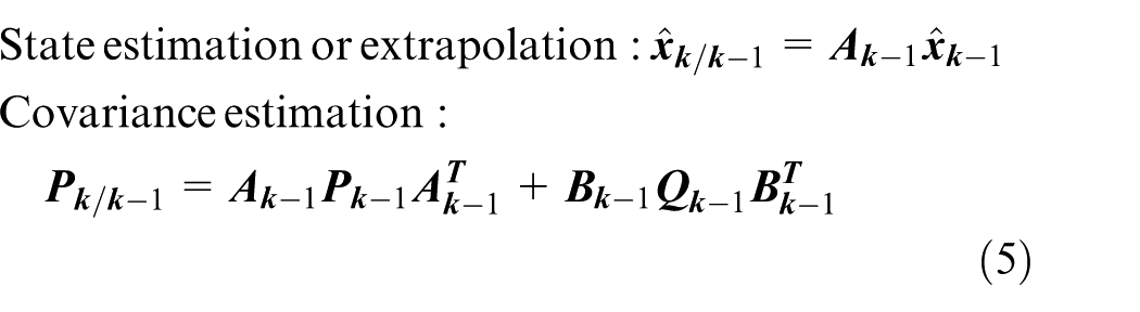
Such calculation will be iterated until the estimated value is equal to or beyond the predefined characteristic parameter threshold. Moreover, the mean and variance of estimation value are defined as the state and covariance estimation mentioned above, that is, at

where

Probability of the dedicated failure prognosis.
Uncertainty source analysis
According to the filtering estimation principle and flowchart in section “Kalman filtering,” the whole prediction process of stochastic filtering–based method can be summarized as shown in Figure 4. 18 The prediction process consists of the following steps:
Data sampling and transferring. Different types of sensors are used to collect corresponding system parameter. Meanwhile, the conversion of various physical signals to electrical signals is required in this step.
Data preprocessing and feature extraction. Data transmitted from sensors will be preprocessed to specified format for subsequent failure prognosis. Simplified, integrated, or compressed data will be the output in this step.
Determining the filtering model. As the different kinds of data have different characteristics, or the same data type in different system stages also has different characteristics, the filtering model of subsequent filtering calculation should be determined specifically.
Stochastic filtering. The system state one-step estimation is completed by the filtering algorithm and flowchart in section “Kalman filtering.”
Failure prognosis. If the system noise is assumed to be zero, and no new information is measured in equation (4), system state in future can be calculated by equation (5) in the probability sense.

Failure prognosis process.
In this process, different uncertainties will be introduced and propagated step by step as shown in Figure 4. Next, the three types of uncertainties derived from different sources will be analyzed in this section.
Model parameter uncertainty
The real system cannot be modeled accurately, and the error of system mathematical model cannot be known in advance. For system state estimation and prediction based on stochastic filter, the system’s model is also completely unknown. Such error can be seen as system model parameter uncertainty. Taking the system description equation (1) as an example, system uncertainty cannot only be expressed by some parameters’ perturbation in system matrix
Measurement noise
Measurement noise or system output noise is the main uncertainty source during the failure prognosis process in a real environment. Environment noise, sensor inaccuracy, transmission noise, and data reduction effect can be seen as measurement noise. These noises can make the measurement result cannot reflect the true value of the measured item.
In terms of different mechanisms of the measurement noise, it can be classified as system error, random error, and gross error. System error is the measurement tool or system’s inherent error, and gross error is the error that is obviously inconsistent with the fact. Random error can be further divided as normal and abnormal distribution errors according to its PDF. In general case, system error and gross error can be removed by mathematical method, and the random error will be assumed to follow normal distribution. However, the statistical characteristic of dynamic noise in real environment is very hard to acquire exactly, and moreover, the initial “white” noise will also be colored as it is transferred through signal channel and preprocessed. This means, in most engineering applications, the measurement noise is only partly known or approximately or even totally unknown.20,21
Failure threshold uncertainty
In the traditional overhaul or maintenance activities, the failure threshold, no matter such threshold value is given by human or intelligent monitor system, is given by experience and fixed in essence. However, it is just a traditional idea and may lead to the neglect of the uncertainty in engineering practice. Such assumption or neglect may not be unreasonable in most cases, as the “point” which the system performance degrades to failure, the failure threshold will be changed with the different operating environments, operators, and the system individual differences. 22 It is a challenging problem to consider the failure threshold’s uncertainty and model the real failure zone. In the sequel, the failure prognosis method with confidence interval will be presented in the next section, which considers the three kinds of uncertainties mentioned above.
Failure prognoses with multiple uncertainty sources
System parameter adaptive filtering
In general, the parameter uncertainty can be solved by the state augmentation; however, such method will increase the calculation, and sometimes, the estimation error will even become worse. For this reason, the idea of the separation of Friedland 23 estimation was introduced in this section: the filtering process is separated robustly as the normal state estimation and system error estimation. For the state–space model in equation (1), it is assumed that there are some parameter perturbations in the system matrix which can be described as

The uncertainty item

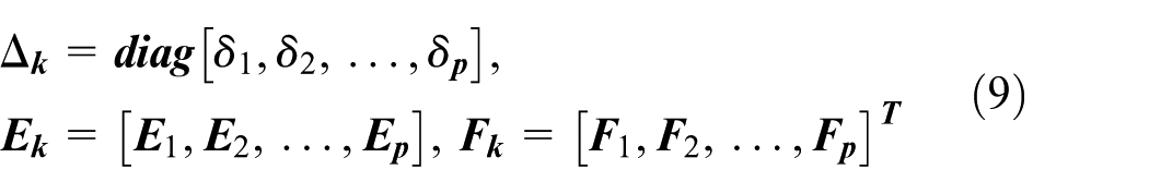
where
To simplify computation, the above three matrices are defined as
With equation (9), system model can be rewritten as

Substituting equation (10) into measurement output expression in equation (1), the output error is
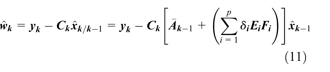
If the uncertainty item
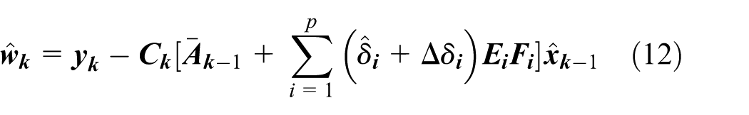
Differentiate equation (12) with every uncertainty item

Set all the uncertainty items as

Based on classical least square recursion, the system parameter update algorithm can be obtained as follows


Based on measurement output error
Robust filters design for unknown measurement noise
System or measurement noise in Kalman filtering process is defined as variance matrices
In all, the gain calculation loop, as shown in Figure 1, which contains the three items (i.e.

Substituting the estimation mean-squared error

where

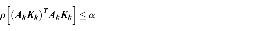
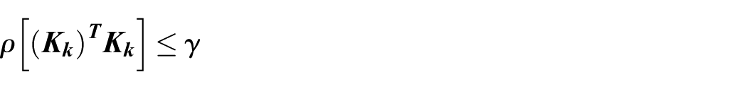
Let

If the spectral radius
Theorem 1
The filter with filtering gain


Proof
With the above derivation, we can conclude that the state estimation error in all steps is acceptable if the following four conditions are valid


These conditions can be transferred to


and they are equal to


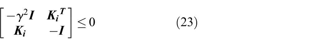
With the Shur formula, 20 LMIs (20)–(23) can be obtained.
Remarks 1
According to our analysis, as the real constants
Failure prognosis with failure threshold distribution
Based on the advanced robust filtering on section “Robust filters design for unknown measurement noise,” the forward failure prognosis value calculation can be started from “current filtering state”


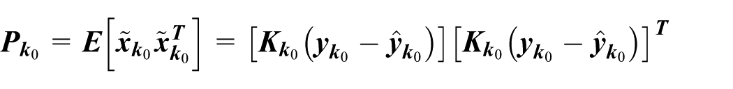
Since there is no variance item in robust filter in section “Robust filters design for unknown measurement noise,” the variance matrix

As shown in Figure 3 in section “Failure prognosis approach,” the cumulative probability of failure before time

where
If the confidence probability is set to

With equations (24), (25), and (27), the failure prognosis value with confidence probability
In general, the actual failure threshold

Remark 2
If the failure threshold follows normal distribution
Failure prognosis value estimation algorithms
In section “Failure prognoses with multiple uncertainty sources,” the probability of system state falling into the failure threshold
Step 1. Initialize the system state
Step 2. Calculate one-step forecasting
Step 3. Calculate the filter gain
Step 4. Get the state estimation as
Step 5. Assume the initial system matrix parameter error is 0 and then update parameter by the parameter identification algorithm in equations (13)–(16).
Step 6. Reset
Step 7. Predict the system’s future state value step by step by equations (24) and (25) and then complete the failure prognosis with predefined failure threshold distribution and failure probability.
Such process can be shown in Figure 5.

Failure prognosis value estimation procedure.
Simulation examples
In this section, the advanced failure prognosis method proposed in this article will be applied to an aircraft fuel feed system simulation case. First, the fuel feed system’s failure modes are analyzed and then the proposed method and other classical methods are used to complete failure prognosis and compare with each other.
Failure effect analysis of fuel feed system
The function of fuel system is to continuously and stably provide engine and auxiliary power unit (APU) with adequate fuel under permitted working conditions and flight states. Modern aircraft fuel feed system consists of electronic control unit, fuel pipeline, and different valves and is a hybrid system with mechanical, electronic, and liquid component, which is shown in Figure 6.

Aircraft fuel feed system diagram.
Each fuel tank has two booster pumps; fuel booster pump extracts fuel and supplies it to the engine feed manifold by pipeline. According to the fuel system operating principle, the component’s performance or reliability on supply line is important to guarantee fuel supply. Booster pump is the key component on supply line, which provides fuel press in most flight stages. In this article, we take the booster pump subsystem as an example.
Booster pump boosts the fuel by its vane’s high-speed rotation, which will introduce cavitation erosion. Under the high-speed flowing and pressure variation condition, the air bubble will be introduced on the vane’s surface as the pressure on the vane is lower than fluid’s steam pressure. And meanwhile, the gas dissolved in fluid may be also separated out to air bubble. After this, the air bubble will be broken as the fluid’s pressure is greater than bubble’s pressure; such sudden action will make huge temperature impact on vane’s surface, which leads to the vane’s fatigue and breaking off or even big pit. Such phenomenon is called cavitation erosion, as shown in Figure 7. Cavitation erosion will decrease the vane area and then makes the pump’s driving force weaker and weaker. Meanwhile, the output pressure will also become smaller and smaller, until it cannot satisfy fuel feed system’s performance index. This means, fuel supply pressure is sensitive to the inner failure mode and can be used to monitor system’s health state.

Vane’s cavitation erosion.
Based on the characteristic parameter simulation output, we can complete the fuel feed system’s failure prognosis with the proposed method. Figure 8 shows the output pressure value of hydraulic booster pump in aircraft fuel feed system with different wear parameters during the whole life period; the x-axis represents system running time, and y-axis shows the pressure values. As shown in Figure 8, during the whole operation cycle, pump’s output pressure value variation presents different degradation trends with different wear conditions. In this figure, the x-axis representing time is operational time (×106 s).
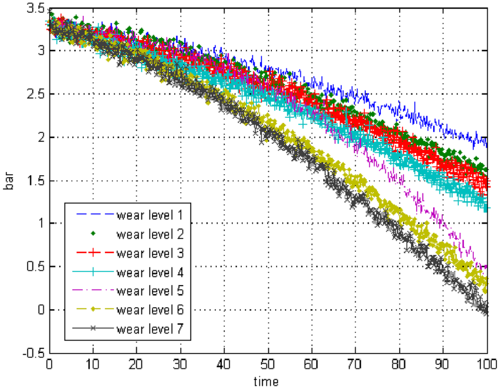
Pressure curves during the whole life period under different wear coefficient conditions.
Parameter adaptive filtering results
As shown in Figure 8, fuel system’s output pressure varies dramatically with the different wear levels. This means, system mathematical model which describes the degradation process also has to be changed; in other words, the actual system’s model has uncertainty factors.
From viewpoint of theoretical model, such variation can be described as perturbation

where

where
In contrast, the classical Kalman filer or nonparameter adaptive filter and parameter adaptive filter are adopted to estimate the actual output pressure data with different wear levels. Figures 9 and 10 and Table 1 illustrate the estimation results’ comparison with different methods.

Comparison of estimation error with different wear levels.

Comparison of estimation results with given wear level.
Mean-squared error of two estimation methods with different wear levels.

Figures 9 and 10 show that the estimation error of nonadaptive filter obviously becomes greater as system workload increases or wear level becomes worse, but the adaptive filter which updates the system parameter in each estimation step is fit for different wear levels and can reduce the estimation error. Obviously, the subsequent failure prognosis case simulation in section “Failure prognosis estimation results” will be affected by these different estimation effects dramatically.
Robust filtering results
The model in equation (29) with unknown noise characteristic or colored noise will be used to verify robust filtering method’s performance. As discussed at the end of section “Failure prognoses with multiple uncertainty sources,” the three parameters
Comparison of absolute estimation error with colored noise condition.

Comparison of absolute estimation error with unknown noise condition.
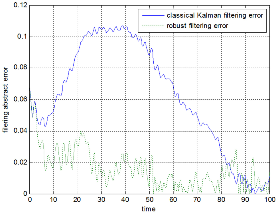
Figure 11 shows the absolute estimation error of the proposed robust filter and classical Kalman filter when system output pressure data have colored noise. With unknown characteristic noise in measured data, Figure 12 illustrates the absolute estimation error for four different filters, which are classical Kalman filter with known noise level, robust filter, classical Kalman filter with unknown noise level, and the H∞ filter. From Figures 11 and 12, the following is clear that
The robust filter is insensitive to colored noise and can guarantee system estimation error better than classical Kalman filter.
The robust filter’s performance is same as classical Kalman filter with known noise level and may be a little better than H∞ filter.
Obviously, robust filter is better than the Kalman filter with unknown noise level.
In summary, for system with unknown noise characteristic, such robust approach can improve estimation efficiency. And the theoretical analysis in section “Failure prognoses with multiple uncertainty sources” is verified by the simulation results.
Failure prognosis estimation results
The approach derived in section “Failure prognoses with multiple uncertainty sources” will be used for failure prognosis of fuel booster pump system. Through the simulation in section “Parameter adaptive filtering results,” we can conclude that the model exhibits good tracking ability for all the testing data, and one of the results is shown in Figure 10.
The adaptive and robust characteristics of the above approach can be used to update the system parameters in the presence of new information and are insensitive to unknown noise. The failure prognosis results with equations (24)–(27) and the deterministic threshold at several time points are plotted in Figures 13–15. In our simulation, the deterministic threshold for booster pump is set at 2 bar, and the confidence probability is 50%.

Comparison of advanced and classical failure prognosis results with single threshold.

Comparison of advanced and classical failure prognosis PDF results at different time point 1.

Comparison of advanced and classical failure prognosis PDF results at different time point 2.
In Figure 13, the solid line is the measured output signal of booster pump pressure, the dash line is real decay parameter’s value, the dot line is parameter prediction zone by advanced failure prognosis estimation method in this article, and the dash–dot line is parameter prediction zone by classical failure prognosis estimation method which is given in section “Fault prognosis theory based on stochastic filtering.” In different time points, the prediction result of our method is fit better than the classical method, and moreover, as shown in Figure 13, the prediction zone of classical method has deviated from the actual failure time point.
Figure 14 illustrates the conditional PDFs for failure prognosis obtained at each time point with different methods, respectively; the bold solid line is the prediction results for advanced method in this article and dash line is for classical method, and meanwhile, the dots represent the actual failure prognosis at the corresponding time point. The two PDFs are obviously different, and the solid ones are narrower than the dash ones which are obtained from the classical method.
Figure 15 shows the plane information about the failure prognosis in different time points. The x-axis indicates the booster pump’s working time, and the y-axis indicates the system failure time. The dot line throughout the upper left corner to the lower right corner in Figure 15 represents the actual system failure time in current time, and the thick solid line is obtained by the failure prognosis points set segment connection, whose points were obtained by the proposed method in this article; similarly, the thick dashed line’s points were obtained by the classical method. In order to show clearly, the PDFs of each failure prognosis point with different methods are given by the dashed line. Obviously, the curves show that the proposed method in this article is more reliable, and the solid line is more fit to the actual failure prognosis line.
In summary, with parameter updating and robust treatment of system estimation in each step, the proposed failure prognosis method which considers multiple uncertainty sources shows better failure prognosis efficiency and accuracy.
From the analysis in section “Uncertainty source analysis,” the actual component’s failure time point always belongs to a failure time interval in the sense of probability due to the complex field environment or device individual difference, rather than a single threshold just like the above simulation, which means that the actual failure threshold may follow some function distribution

Comparison of failure prognosis PDF results with single threshold and threshold zone.
Similar to Figure 14, the dots represent the actual failure prognosis at the corresponding time point, and of course, the failure prognoses by the two methods which consider or do not consider threshold distribution contain such points. As current time point moving, the curves become narrow and the failure prognosis results become more credible. For the first curve set, the two results near the time 40 (bold solid line for single threshold and dash line for another) are almost the same because of failure time is far from current time, and there is only a little information available for prediction. However, as the time point moving, the two results become more different gradually. Figure 16 shows that compared with the failure prognosis with single threshold, the introduction of threshold distribution will reduce component’s unnecessary early replacement.
Conclusion
In this article, a failure prognosis approach with multiple uncertainty sources has been presented. Such approach utilizes adaptive updating scheme, robust filter, and total probability formula to form the advanced failure prognosis tool which can predict the residual life based on the measured data. The fault prognostic process was listed in section “Failure prognosis value estimation algorithms” to simplify the actual use of such approach.
Simulated results for the fuel feed system’s booster pump showed the validity of the proposed method. Further research should be focused on future usage uncertainty which has relationship with maintenance decision, and another meaningful area is the real engineering environment, which will perform its significant value in maintenance or logistics support.Furthermore, we would like to see the proposed failure prognosis approach can be used in flight control problems.26–28
Footnotes
Academic Editor: Yongming Liu
Declaration of conflicting interests
The author(s) declared no potential conflicts of interest with respect to the research, authorship, and/or publication of this article.
Funding
The author(s) disclosed receipt of the following financial support for the research, authorship, and/or publication of this article: This work was partially supported by National Natural Science Foundation of China (61304098, 61622308), Natural Science Basic Research Plan in Shaanxi Province (2016KJXX-86) the Fundamental Research Funds for the Central Universities (grant nos 3102014JCQ01010 and GK201302004), the Project Supported by Natural Science Basic Research Plan in Shaanxi Province of China (program no. 2015JQ6255), International Science & Technology Cooperation Program of China (grant no. 2014DFA11580) and Fundamental Research Funds of Shenzhen Science and Technology Project under grant JCYJ20160229172341417.