Sage Journals: Discover world-class research

Abstract

Common control systems for mobile robots include the use of some deterministic control law coupled with some pose estimation method, such as the extended Kalman filter, by considering the certainty equivalence principle. Recent approaches consider the use of partially observable Markov decision process strategies together with Bayesian estimators. These methods are well suited to handle the uncertainty in pose estimation but demand significant processing power. In order to reduce the required processing power and still allow for multimodal or non-Gaussian uncertain distributions, we propose a scheme based on a particle filter and a corresponding cloud of control signals. The approach avoids the use of the certainty equivalence principle by postponing the decision on the optimal estimate to the control stage. As the mapping between the pose space and the control action space is nonlinear and the best estimation of robot pose is uncertain, postponing the decision to the control space makes it possible to select a better control action in the presence of multimodal and non-Gaussian uncertainty models. Simulation results are presented.

Keywords

Mobile robotics particle filter nonlinear control stochastic control stochastic estimation

Introduction

Mobile robots are known to be subject to uncertainty in both the robot behavior and the environment where the robot navigates. Additionally, the availability of sensors capable of characterizing the environment is, in general, an unsolved problem. These issues can be modeled by a stochastic system. The classic approach for state estimation and control of stochastic systems is to consider the expected value of the system state variables and the certainty equivalence principle.^1,2 Expected value approaches, however, cannot be used when multimodal (or even skewed) distributions are present. On the other hand, skewed or multimodal distributions can arise due to sensor fusion and other typical mobile robotics problems.³ Also, nonlinear dynamics often generate multimodal or skewed distributions from normal or uniform distributions. The current state-of-the-art approach to cope with uncertainties, especially those with non-Gaussian probability distributions, is to use Bayesian filters to estimate the system state and then compute a control signal based on the result of the estimation procedure, which is a probability density, a histogram, or a set of particles or probabilities over a topological map. This signal can be obtained from a mode or through optimization, such as partially observable Markov decision processes (POMDP) approaches.^4,5 The use of POMDP for systems with continuous states demands approximations, or the problem becomes intractable.³

This article proposes a control scheme for a differential-drive mobile robot that maps a set of possible states into a space of control signals. Both the state transition and observations are subject to uncertainty. Hence, a particle filter is proposed for state estimation. However, contrariwise to the usual approach, the resulting state estimate is not taken to be a single point in the state space, but the full cloud of particles which represents the probability of each estimated particle to be the true state. Then, a globally stable control law is considered for the mapping of the cloud of particles in state space into a cloud of particles in control space. Then, the control signal to be applied to the robot is chosen as one of those in the most populated regions in the control space.

In other words, the proposed method avoids to decide the robot pose and then compute the control signal to correct it, but instead, postpones the decision to the control stage. The traditional approach (at least for low-level control) is to use the particle filter to solve the localization problem which gives a best estimation of the robot pose and then use this pose to compute the control action. As the mapping between the pose space and the control action space is nonlinear and the best estimation of robot pose is uncertain, postponing the decision to the control space makes it possible to select a better control action as many not-so-good pose estimatives could be mapped to the same control action giving it a higher probability to be a better control action. This capability is important in the case of multimodal and non-Gaussian uncertainty models.

Furthermore, the sensor observations are restricted in sampling frequency, in the sense that an absolute pose measurement, which was assumed to be obtained from a GPS, is only available on same control cycles, while dead-reckoning information from encoder measurements is available in all control cycles.

A description of the robot is presented in section “Robot model.” The proposed control method is explained in sections “Pose estimation by particle filter” and “Control using a cloud of particles.” More specifically, section “Pose estimation by particle filter” explains the pose estimation based on a particle filter and section “Control using a cloud of particles” presents the control method based on the cloud of particles. Results are presented in section “Simulation results” and final remarks and suggestions for future development are presented in section “Conclusions.”

Robot model

Consider a differential-drive mobile robot, with the coordinate systems shown in Figure 1, where the $(X_{c_{1}}, X_{c_{2}})$ coordinate system is attached to the robot and (X₁, X₂) is the inertial coordinate system. In continuous time, the kinematic model of the mobile robot, moving on a horizontal plane, is described by

Figure 1.

Differential-drive mobile robot coordinates.

\dot{x} = f (x, u) = [\begin{matrix} \cos x_{3} & 0 \\ sin x_{3} & 0 \\ 0 & 1 \end{matrix}] u

where $x = {[\begin{matrix} x_{1} & x_{2} & x_{3} \end{matrix}]}^{T}$ is the state vector and $u = {[\begin{matrix} u_{1} & u_{2} \end{matrix}]}^{T}$ is the control vector. The state variables x₁ and x₂ are the position coordinates, x₃ is the orientation angle, and the control variables u₁ and u₂ are the linear and angular velocities.

By supposing a zero-order holder on the control inputs, the trajectories of the discretized version of equation (1) are circumference arcs and the robot orientation is tangent to the arc as shown in Figure 1 and given by

x (k + 1) = f_{d} (x (k), u (k)) = x (k) + [\begin{matrix} T u_{1} (k) [sync (\frac{T u_{2} (k)}{2}) \cos (x_{3} (k) + \frac{T u_{2} (k)}{2})] \\ T u_{1} (k) [sync (\frac{T u_{2} (k)}{2}) sin (x_{3} (k) + \frac{T u_{2} (k)}{2})] \\ T u_{2} (k) \end{matrix}]

where $s y n c (x) ≜ \frac{sin (x)}{x}$ and T is the sampling period.

However, imperfections due to the type of terrain, differences in wheel sizes, geometry of the robot, wheel slipping, and others affect the actual trajectory, which differs from the ones described by either equation (1) or (2). Furthermore, common assumptions such as that the velocity is known with absolute accuracy, instantaneous computation of control signals, and constant sampling period do not actually hold. Hence, the robot behavior can be better described by stochastic models, as proposed by Thrun et al.⁵ and Rekleitis.⁶ These models account for two types of errors, in fact: systematic errors and nonsystematic errors. Systematic errors can be compensated for by appropriately calibrating the parameters of the model.^6,7 However, nonsystematic errors are due to stochastic effects and cannot be compensated for by calibrating.

The stochastic effects can be observed in the robot motion by drifting robot with respect to the nominal trajectory in both traveled distance and orientation. By drifting, those errors increase with time, and therefore, they are modeled as uncertainty in linear and angular velocities of the robot. Furthermore, the stochastic effects are closely related to the linear velocity of the model.⁶ Hence, the stochastic version of equation (1) is

\dot{x} (t) = f (x (t), u (t) + w (t))

with $w (t) = u_{1} (t) {[w_{t} (t) w_{D} (t)]}^{T}$ , where $w_{t} (t) \sim N (0, σ_{t}^{2})$ and $w_{D} (t) \sim N (0, σ_{D}^{2})$ are Gaussian processes representing the uncertainty in linear and angular speeds, respectively.

It must be noted that while w(t) are read as addends in equation (3), it is not an additive uncertainty, since it depends on the linear speed u₁ and f(⋅, ⋅) is nonlinear. Also, even though w_t(t) and w_D(t) are assumed to be Gaussian, the resulting state x(t) is not Gaussian, due to nonlinearities.

An equivalent discrete model could be obtained by considering a discrete uncertainty w(k) similar to w(t) added to u(k) in equation (2). However, that would lead to a model where, even under uncertainty in u(k), the orientation at k + 1 would remain tangent to the trajectory of the robot. Therefore, that model would not be able to properly represent uncertainty in orientation at k + 1, which could be nontangent to the robot trajectory as shown in Figure 2(a).

Figure 2.

Discrete-time system transition. (a) Deterministic system and (b) stochastic system.

In order to obtain a discrete model that can properly represent the orientation uncertainty at k + 1, it can be assumed⁶ that half of the effects of the uncertain angular velocity acts through the state transition, therefore affecting both position and orientation at k + 1, and the other half acts directly on the orientation at k + 1. Hence, the uncertainty w_D(t) in the continuous model is represented by two uncertainties in the discrete model $w_{d_{1}} (k) \sim N (0, σ_{d}^{2})$ , which acts through the state transition and $w_{d_{2}} (k) \sim N (0, σ_{d}^{2})$ , which acts directly on state at k + 1. The effects of w_t(t) can be directly mapped in $w_{t} (k) \sim N (0, σ_{t}^{2})$ . Then, the discrete model can be written as

x (k + 1) = f_{d} (x (k), u (k) + w_{1} (k)) + w_{2} (k)

where the state transition f_d(⋅, ⋅) is given by equation (2) and

w_{1} (k) ≜ u_{1} (k) [\begin{matrix} w_{t} (k) \\ w_{d_{1}} (k) \end{matrix}], w_{2} (k) ≜ T u_{1} (k) [\begin{matrix} 0 \\ 0 \\ w_{d_{2}} (k) \end{matrix}]

Since $w_{d_{1}} (k)$ and $w_{d_{2}} (k)$ are assumed to represent half of the effects of w_D(t), their variances should be the half of $σ_{D}^{2}$ or

σ_{d} = \frac{σ_{D}}{\sqrt{2}}

The state transition is illustrated in Figure 2(a), where both the arc distance and angle are affected by w₁(k) and the final orientation is also affected by w₂(k) (compare to Figure 2(b)). It must be noted that while w₁(k) and w₂(k) are read as addends in equation (4), they are not actually additive uncertainty, since they depend on the linear speed u₁(k) and f_d(⋅, ⋅) is nonlinear.

As Figure 2(a) shows, the model (equation (4)) describes the state transition as circumference arcs with stochastic length and angle, with an added orientation uncertainty. This model will be used for estimating the state transitions for a set of possible values for the state vector, as explained in detail in section “Pose estimation by particle filter.” It is important to note that even though w_t(k), $w_{d_{1}} (k)$ , and $w_{d_{2}} (k)$ are assumed to be Gaussian, the resulting state x(k + 1) is not Gaussian, due to nonlinearities. The equation (3) is used to simulate the robot in section “Simulation results,” while equation (4) is used for state estimation.

Pose estimation by particle filter

Mobile robots suffer from several sources of uncertainty. Their sense of awareness of the surrounding environment is limited not only by the sensors it is equipped with but also by its ability to process and act based on the information provided by the observations from these sensors.^5,7 These are also limited in the sense that not all sensors can return an observation at the same rate.

The state of a mobile robot is not readily available and must be estimated from sensor observations. In general, the observation vector, y(k), is corrupted by noise v(k), that is

y (k) = h (x (k), v (k))

In this article, we consider digital incremental encoders on the wheels and a GPS sensor. The method, however, could be extended to consider more and other types of sensors, just by considering them in the definition of $h (x (k), v (k))$ . The measurements from the incremental encoders provide information about the robot current pose (i.e. position and orientation) relative to its previous one, while the observation from GPS provides a measurement with respect to an inertial reference frame. Encoder observations are angular displacements of the wheels which are measured at each sampling instant. These are mapped to relative linear and angular position displacements, which in turn are mapped to linear and angular velocities, assumed to be constant between sampling instants. Thus, we assume that u(k) can be measured from the encoder observations, while other sensors are used to form the system observation equation (5). For the sake of simplicity, we assume here that only a GPS is used in addition to incremental encoders. The GPS system gives sparse (time wise) information about global positioning through the observation vector y(k), but it is corrupted by observation noise v(k)

y (k) = C x (k) + v (k)

with C = I, the identity matrix.

Note that for other types of sensors, the mapping from x(k) and v(k) to y(k) can be nonlinear and that when redundant sensors are used, the dimension of y(k) may be greater than that of x(k).

Data from sensors are integrated by a particle filter for a pose estimate represented by a set of particles. Particle filters belong to a family of estimation methods known as Bayesian estimators. Bayesian estimators aim to consider the uncertainty of both state transition and system observations in order to provide a realistic result. In accordance with the uncertainty approach in metrology,⁸ the estimation result is extended so as to include information other than a single value, to be attributed to the quantity being measured. The most comprehensive result of an estimation is a (joint) probability distribution function of the state vector, considered at each sampling instant. These have either one of two disadvantages: requiring an analytic solution of the Bayes filter equations or requiring an infinite number of parameters to be fully described. Kalman filters are able to, under appropriate assumptions, generate an analytic solution in the form of a multivariate Gaussian distribution. This makes it possible to summarize the data as a mean vector and a covariance matrix. Therefore, the resulting probability density can be finitely parameterized. However, for nonlinear systems or uncertainties that cannot be expressed as a Gaussian parcel added to the state transition, such analytic solution cannot be obtained and the estimation result cannot be expressed using a finite set of parameters. General Bayesian estimators provide a density function or an approximation of it but require high processing power and memory. Particle filters are an efficient approximation which returns a set of particles as possible values for the state vector at each sampling instant, instead of an analytic function.

As is the case for many Bayesian filter techniques, particle filter algorithms can be viewed as composed of two stages called prediction and update. This last step is also called resampling or importance sampling.

The particle filter scheme is summarized below. A more detailed presentation is available in the work done by Thrun et al.⁵

At each sampling instant, possible values for the state vector x_i(k), $i \in [1, M]$ , are considered, based on the previous observations from the system. Each vector x_i(k) is called a particle and M is the total number of particles. The state belief ${bel}_{p} (x (k))$ is given by the set of all such particles, that is

{bel}_{p} (x (k)) = {x_{1} (k), x_{2} (k), \dots, x_{M} (k)}

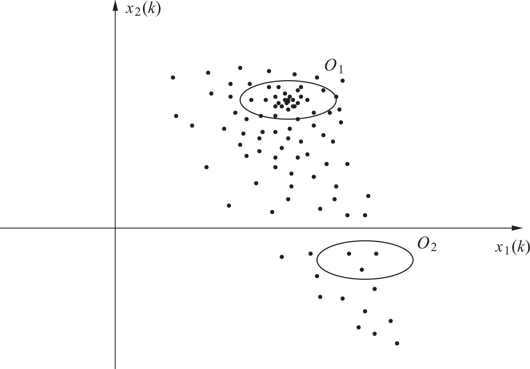
The state belief is an approximation of a probability density function in the following sense: State space regions with a relatively large number of particles have high probability density values, while regions with relatively few particles are supposed to have low density values. Figure 3 shows an example of a state belief given by particles for a second-order system, where the region $O_{1}$ has a high probability of containing the system state and a region $O_{2}$ has a relatively low probability of containing the state of the system.

Figure 3.

Example of state belief for a second-order system and two regions $O_{1}$ and $O_{2}$ with different probabilities of containing the state.

The prediction step of the algorithm takes the state belief and the system input (control) vector as arguments to generate the prior state belief ${\bar{bel}}_{p} (x (k + 1))$ . For each particle, a new one is generated, according to the state transition function of the system equation (4), with the uncertain terms obtained from pseudo-random number generators with the appropriate distributions. Note that this can be done for any distribution. The prior state belief is

{\bar{bel}}_{p} (x (k + 1)) = {x_{1} (k + 1), x_{2} (k + 1), \dots, x_{M} (k + 1)}

where each particle $x_{i} (k + 1)$ , $i \in [1, M]$ , is obtained as

x_{i} (k + 1) = f_{d} (x_{i} (k), u (k) + w_{1_{i}} (k)) + w_{2_{i}} (k)

Figure 4 shows three prediction steps from a set of 50 particles with input $u = {[\begin{matrix} 2 & 0.8 \end{matrix}]}^{T}$ , with the initial set of particles at the origin. It can be observed that the particles move apart in fan shape, which results from the uncertain terms.

Figure 4.

Predicted particles for three steps with null initial conditions and $u {= [2 0.8]}^{T}$ .

The set of particles ${\bar{bel}}_{p} (x (k + 1))$ is obtained without information from the system observation at k + 1: It takes only the set of particles $be l_{p} (x (k))$ and the input signal as arguments. This set of particles should be updated with the information from the observations, returning the updated state belief ${bel}_{p} (x (k + 1))$ at k + 1. This is accomplished by obtaining the importance factor $ι_{i} (k + 1)$ for each particle $x_{i} (k + 1)$ according to

ι_{i} (k) = f_{y} (y (k) | x_{i} (k))

where $f_{y} (y (k) | x (k))$ is the conditional probability density function of y(k) based on the knowledge of the state vector x(k).

In this article, it was assumed that the GPS observation noise v(k) is jointly normally distributed, with zero mean and covariance matrix $P$ . Since $y (k) = C x (k) + v (k)$ , we have that

f_{y} (y (k) | x (k)) = \frac{e^{(- \frac{1}{2} {[y (k) - C x (k)]}^{T} P [y (k) - C x (k)])}}{\sqrt{{(2 π)}^{n} | P |}}

where n is the number of rows of y(k).

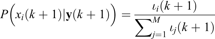
The observation y(k) and the particles $x_{i} (k)$ are known, therefore, $ι_{i} (k)$ can be computed as a deterministic number. The importance factor is proportional to the likelihood of the robot being at a neighborhood of the respective particle. Then, the updated state belief $be l_{p} (x (k + 1))$ is obtained by selecting in ${\bar{bel}}_{p} (x (k + 1))$ the particles with a probability $P (x_{i} (k + 1) | y (k + 1))$ proportional to its importance factor, according to

P (x_{i} (k + 1) | y (k + 1)) = \frac{ι_{i} (k + 1)}{\sum_{j = 1}^{M} ι_{j} (k + 1)}

until M particles are selected. Each particle selection is independent of the previous one. Hence, some particles from the prior state belief are not included in the current belief, while others, usually those with higher importance factors, are included more than once.

The belief update demands an observation to take place. In this article, a GPS was considered to have a sampling period larger than that of the incremental encoders. As a result, the update step does not occur at every sampling instant, but only when the observation from the GPS is available.

Control using a cloud of particles

Differential-drive mobile robots are nonholonomic systems.⁹ For this type of system, it is hard to steer the state to any fixed point in the space due to limited state manipulability from the inputs. This is easy to verify by inspecting equation (1), taking the inputs to be either u₁ = 1 and u₂ = 0 or u₁ = 0 and u₂ = 1. The first situation has the robot moving in the same direction of the wheels, which affects the first two state variables, while the second one results in a pure rotation around its axis, which affects the third one. These cannot be combined to obtain instant velocity that is not also along the direction of $X_{c_{1}} (k)$ (see Figure 1). In spite of this, the system is controllable.¹⁰ It can be shown that as a consequence of the Brockett conditions,¹¹ it is not possible to asymptotically stabilize the system at an arbitrary point through a time-invariant, smooth state feedback.

Ways around Brockett’s conditions to obtain asymptotic stability are time-variant control,^12

–15 nonsmooth control,^10,16,17 and hybrid control laws.¹⁸ These can be used for low-level control, which is the task of moving a robot either to a location or along a defined trajectory, with no consideration about why it should do so. In this article, we will obtain a set of possible control signals based on a nonsmooth control law. A general way of designing control laws for nonholonomic systems through nonsmooth coordinate transformations was presented by Astolfi.¹⁰

The mappings from the system state to the control space which are used for point stabilization are such that the state space origin is made asymptotically stable. If we represent the mapping as $g : X \to U$ , $x \in X$ , and $u \in U$ , then the autonomous system

\dot{x} = f (x, g (x))

where f(⋅, ⋅) described by equation (1) is asymptotically stable at the origin. However, it is desired to stabilize the robot at any point x_r, which means any given position and orientation $(x_{r_{1}}, x_{r_{2}}, x_{r_{3}})$ . This can be done by the coordinate change $\bar{x} (x, x_{r})$ , obtained by setting a new reference frame $X_{r_{1}} X_{r_{2}}$ at the reference position $(x_{r_{1}}, x_{r_{2}})$ with an angle $x_{r_{3}}$ , as shown in Figure 5. Thus, the coordinate change from X₁X₂ to $X_{r_{1}} X_{r_{2}}$ consists of a translation and a rotation of angle $x_{r_{3}}$ . It is readily verified that ${\bar{x}}_{3} = x_{3} - x_{r_{3}}$ . Therefore, the coordinate change $\bar{x} (\cdot, \cdot)$ is given by the transformation

Figure 5.

Robot coordinates with respect to the reference frame.

\bar{x} = [\begin{matrix} R (x_{r_{3}}) & 0 \\ 0 & 1 \end{matrix}] (x - x_{r})

where $R (x_{r_{3}})$ is a 2-D rotation matrix, that is

R (x_{r_{3}}) = [\begin{matrix} \cos x_{r_{3}} & sin x_{r_{3}} \\ - sin x_{r_{3}} & \cos x_{r_{3}} \end{matrix}]

Hence, if the system $\dot{\bar{x}} = f (\bar{x}, g (\bar{x}))$ is stable at $\bar{x} = 0$ , then $\dot{x} = f (x, g (x))$ is stable at $x = 0$ . Therefore, in order to stabilize the system at any arbitrary point $x_{r}$ based on a control law g that leads the state to the origin, it suffices to use $g (\bar{x})$ .

Low-level mobile robot control schemes usually take the state vector as input. However, here, the estimation result is a set of particles. This resulting estimation may have points grouped around different regions, as a result of multimodal beliefs. As a consequence, either a mean squared estimation or the expected value is not an appropriate estimation result, and the certainty equivalence principle cannot be applied. We present a way of generating a control signal from the current belief by considering the resulting signal from each of the belief particles and verifying their distribution in the space of the control inputs. This way, not only an appropriate action can be found, but it can be reasoned whether an action is appropriate at a given instant, depending on the resulting set of control particles.

At each sampling instant k, the current belief $be l_{p} (x (k))$ represents possible values for the state vector – the particles. For each particle x_i(k), a control signal u_i(k) is obtained as

u_{i} (k) = g ({\bar{x}}_{i} (k))

with ${\bar{x}}_{i} (k)$ computed by equation (10), leading to

be l_{p} (u (k)) = {u_{1} (k), u_{2} (k), \dots, u_{M} (k)}

where $g ({\bar{x}}_{i} (k))$ is an appropriate mapping from the state space to the space of control inputs.

For each particle, a coordinate change given by Barros and Lages^19,20 is considered

e = \sqrt{{\bar{x}}_{1}^{2} + {\bar{x}}_{2}^{2}}

ψ = atan 2 ({\bar{x}}_{2}, {\bar{x}}_{1})

α = {\bar{x}}_{3} - ψ

Then, the equation (1) can be rewritten as

{\begin{array}{l} \dot{e} & = u_{i_{1}} \cos α \\ \dot{ψ} & = u_{i_{1}} \frac{sin α}{e} \\ \dot{α} & = - u_{i_{1}} \frac{sin α}{e} + u_{i_{2}} \end{array}

Given a Lyapunov candidate function

V = \frac{1}{2} λ e^{2} + \frac{1}{2} (α^{2} + h ψ^{2})

it can be shown that the input signal u_i(k)

u_{i_{1}} = - γ_{1} e \cos α

u_{i_{2}} = - γ_{2} α - γ_{1} \cos α \frac{sin α}{α} (α - h ψ)

with h, γ₁, and γ₂ > 0, makes equation (15) asymptotically stable.^19,20 As a consequence, the input belief contains control signals related to point stabilization of the state particles under no state transition uncertainty, that is to say, assuming a deterministic system with known parameters. Note that even though equation (15) is discontinuous at the origin, due to e in the denominator, the closed loop system is not. The term in the denominator is canceled in closed loop because equation (16) contains e as a factor. For simplicity and easy of analysis, in this article, only the kinematic model of the robot was used. However, the control law equations (16) and (17) can be extended to include the dynamics of the mobile robots. See the work done by Barros and Lages^19,20 for details.

The input belief, obtained by computing equations (16) and (17) for each state particle, cannot be considered a result of the control scheme the way the state belief can for estimation, as it is obvious that the system takes a single two-dimensional vector as input. On the other hand, while an appropriate input vector could be any at a neighborhood of the input particles, we have the input belief as a discretization of an infinite set of possible inputs in a fashion similar to the state belief as a simplification for an infinite set of possible state vectors. As a result, it makes sense to restrict the search and decision regarding an input vector among the ones which belong to $be l_{p} (u (k))$ .

The criterion for choosing an input vector among ${bel}_{p} (u (k))$ considered in this article is to select the one with most local support. This means choosing the one whose neighborhood contains the most values also among ${bel}_{p} (u (k))$ . The neighborhood of each input vector u_i(k) was chosen as an ellipsoidal region S_i, centered at u_i(k), given by

S_{i} = {u (k) : \frac{{(u_{1} - u_{i_{1}})}^{2}}{a_{1}^{2}} + \frac{{(u_{2} - u_{i_{2}})}^{2}}{a_{2}^{2}} < 1}

where a₁ and a₂ are the ellipsoid radii.

The ellipsoid form is based on input limits for wheel velocities. As the input selection happens in the control input space, a particle is selected based on locally supported control signals in that space. That is, regardless of where the respective state particles are located in the state space.

The input restrictions are defined based on the limits for the speed of each of the wheels, as in Alves and Lages.²¹ The set of possible input signals is illustrated in Figure 6.

Figure 6.

Input restrictions. The hatched region is the set of possible input signals so as to satisfy wheel speed limits.

Simulation results

The simulated robot was modeled as the continuous-time stochastic system equation (3), with the state evolution obtained by a fourth-order Runge–Kutta with four steps at each sampling instant. For the particle filter prediction step, the robot was modeled as a discrete-time stochastic (nonlinear) system, described by equation (4). The values of the noise parameters σ_t and σ_D were set as 0.005 and 0.1745 rad/m, respectively. The observation covariance matrix is $P = diag (σ_{y_{1}}, σ_{y_{2}}, σ_{y_{2}})$ , with $σ_{y_{1}} = σ_{y_{2}} = 0.1 m$ , and $σ_{y_{3}} = 1 °$ . The maximum speed the wheels can achieve is 0.471 m/s. The control sampling period T is 50 ms and the GPS output period is 200 ms. A total of 900 particles were used for the estimation and the initial set is composed by equally spaced particles inside a square of 1 m² centered at x(0). The controller parameters were γ₁ = 0.5, γ₂ = 0.5, and h = 1.0. The ellipsoid radii related to u₁ and u₂ are 0.05 and 0.2, respectively. The initial position is $x (0) = {[\begin{matrix} 4 & 0 & π \end{matrix}]}^{T}$ and the reference pose x_r is ${[\begin{matrix} 1.0 & 3.0 & - π / 2 \end{matrix}]}^{T}$ .

At each sampling instant, the state belief is predicted. In the initial state belief, the particles are uniformly distributed in space.

The belief update is done when the observation from the GPS is available. Else, there is no further information and the prior belief is taken as the current belief. The first update takes place in k = 3. A plot of the prior belief ${\bar{bel}}_{p} (x (3))$ in the X₁ × X₂ plane is shown in Figure 7. Again, orientation is omitted for the sake of clearness. A careful inspection will reveal that the particles are not exactly uniformly spaced as in the initial belief. This happens because the particles are predicted through the model equation (4), including a simulation of the uncertainties.

Figure 7.

Predicted state belief at k = 3 in the X₁ × X₂ plane. Orientation is omitted.

The updated state belief at k = 3 is shown in Figure 8(a) and a plot of updated belief in the X₁ × X₂ plane is presented in Figure 8(b) for easier comparison with Figure 7.

Figure 8.

Updated state belief at k = 3. (a) 3-D view and (b) X₁ × X₂ plane. Orientation is omitted.

A number of particles present in ${\bar{bel}}_{p} (x (3))$ (Figure 7) are not included in ${bel}_{p} (x (3))$ (Figure 8(b)) due to resampling. However, some other particles present in ${bel}_{p} (x (3))$ (probably those with higher importance factor) are repeated, also due to resampling.

It has been observed that the update step demands significantly more time (see Table 1) than the prediction. This happens because the prediction model equation (4) is relatively simple, hence the prediction is a straightforward step: a single action is required for each particle. On the other hand, the update is done in two separate steps: the calculation of the importance factors, which has a computational complexity that is proportional to the number of particles, and a further resampling, which requires ordering a vector and finding the position index of values inside it. However, those timings were obtained in a Matlab implementation running in a single core computer. A proper implementation in C or C++ using a multicore machine would be much faster. The calculations have been carried out in Matlab release 2010bSP1 running on an AMD Athlon 64 machine at 3.0 GHz running the Linux operating system. Matlab has to interpret code before executing it and the implemented algorithm was not implemented with parallelization in mind.

Table 1.

Average computation time for each control method steps.

Prediction (ms)	Update (ms)	Control selection (ms)
70	360	940

The set of control signal particles is obtained from the current belief. This has a much different shape than the state belief, as the mapping from states to control signals is done through a discontinuous coordinate transformation, which then is subject to a nonlinear control law.

The control belief at k = 0 is presented in Figure 9(a). As the particles from the initial state belief are uniformly distributed in space, the resulting control belief keeps part of that structure. At the next sampling instant (k = 1), the new state belief, which resulted from the stochastic model assumed for the state transition, is used to compute a new control belief, shown in Figure 9(b).

Figure 9.

Input belief. (a) k = 0 and (b) k = 1.

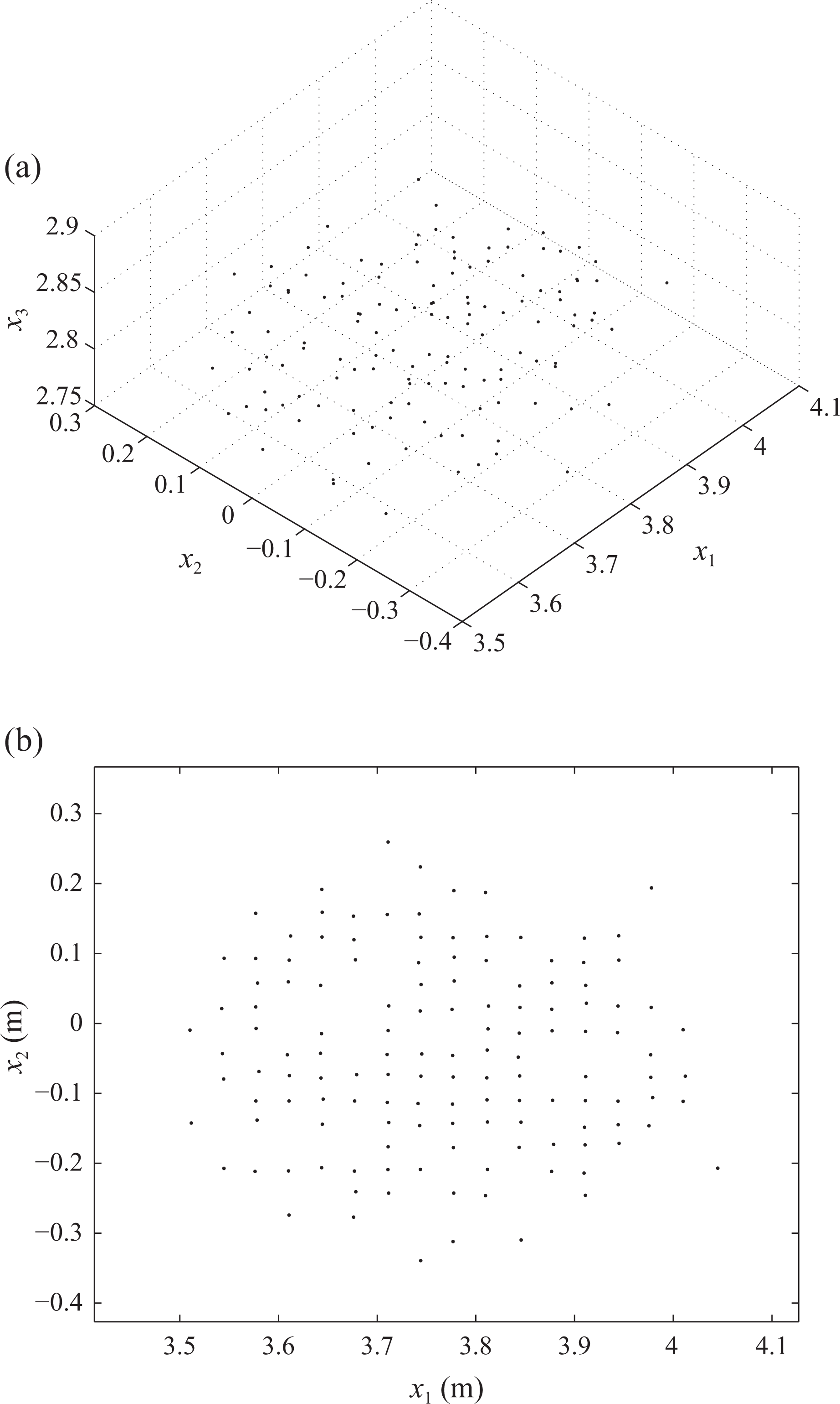
The state belief at k = 50 is presented in Figure 10(a). Figure 10(b) shows its plot in the X₁ × X₂ plane with orientation omitted. The corresponding input belief is shown in Figure 11. Note that the particles are concentrated in smaller regions.

Figure 10.

(a) State belief at k = 50 and (b) its projection in the X₁ × X₂ plane. Orientation is omitted.

Figure 11.

Input belief at k = 50.

A control signal is selected as the particle that maximizes the number of other particles in its neighborhood, as explained in section “Control using a cloud of particles.” While most of them are related to state particles inside a neighborhood of each other, this is not always true as $g (x (k))$ is nonlinear and discontinuous. This action can be understood as maximizing the number of vector states that would be driven similarly to the behavior of a deterministic system. Also note that this is an approximation of taking a value related to a region of high probability density, as the particles are an approximation of a continuous joint probability density function by random sparse values. Figure 12 shows the control signals with respect to time.

Figure 12.

Control signals with respect to time.

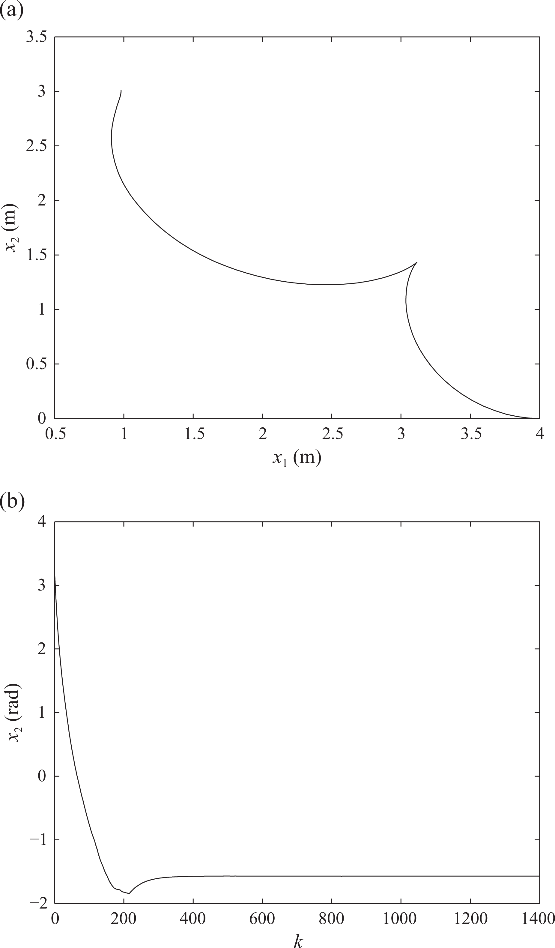
The trajectory of the robot on the plane is presented in Figure 13(a). The state-input mapping is such that the robot approaches the reference with small angle error and negative linear speed (see Figure 12). This happens due to equations (12) and (13), which forces e > 0 and given that the Lyapunov function has a quadratic term in φ. The final position of the robot in Figure 13(a) is $x (k) = {[\begin{matrix} 1.044 & 3.090 & - 1.571 \end{matrix}]}^{T}$ . Figure 13(b) displays the orientation angle with respect to time.

Figure 13.

(a) Robot trajectory on the horizontal plane and (b) orientation angle with respect to time.

The experiment has been repeated in order to verify the stochastic effects in steady state. Particularly, the experiment has been reproduced 50 times and the final state position has been recorded. The mean and standard deviation of the state at the last sampling instant are presented in Table 2.

Table 2.

Final position mean and standard deviation for $x (0) = [4 0 π]^{T}$ and $x_{r} = [1 3 - π {/ 2]}^{T}$ .

State	Mean	Standard deviation
x₁ (m)	0.9973	0.0203
x₂ (m)	3.0027	0.0139
x₃ (rad)	−1.5708	0.0014

Finally, a number of initial conditions have been considered. The trajectories for eight different initial conditions, given by

\begin{array}{l} x (0) = {[4 2 2.5]}^{T} x (0) = {[4 4 3]}^{T} \\ x (0) = {[2 6 1.9]}^{T} x (0) = {[0 6 2.9]}^{T} \\ x (0) = {[- 2 4 π]}^{T} x (0) = {[- 2 2 0]}^{T} \\ x (0) = {[0 0 2]}^{T} x (0) = {[2 0 1]}^{T} \end{array}

are shown in Figure 14(a), and a detail around the reference position is shown in Figure 14(b). The × denotes the final point of the trajectory at k = 1400. It can be observed that the asymptotic convergence which exists in the deterministic and observable case is downgraded to convergence to points in a neighborhood of the reference in the presence of noise and with limited observations. Note, however, that the standard deviation of the final point is consistent with those of the uncertainties, given by σ_t and σ_D.

Figure 14.

Trajectories for eight different initial conditions. (a) Trajectory and (b) detail around the final reference point.

The control signals with respect to time for the eight cases are shown in Figure 15. It can be seen that there are a few peaks. These occur due to the state belief update, which sometimes selects particles from some other region, depending on the last observation.

Figure 15.

Input signals with respect to time.

Again, the experiment has been repeated many times to verify the consistence of the results despite the stochastic effects. The experiment for each initial condition was repeated five times for a total of 40 different trajectories. The final poses have been recorded, and their mean and standard deviation at the last sampling instant are presented in Table 3.

Table 3.

Final position mean and standard deviation for different initial conditions and $x_{r} = [1 3 - π / 2]^{T}$ .

State	Mean	Standard deviation
x₁ (m)	1.0026	0.0212
x₂ (m)	2.9949	0.0109
x₃ (rad)	−1.5706	0.0014

Conclusions

A method for controlling a differential-drive mobile robot through output feedback has been proposed. While only simulation results have been presented, a realistic model for the robot has been used. The system behavior and the information that can be obtained from sensors are subject to uncertainties which are present in mobile robot applications. Furthermore, there are the natural difficulty of controlling nonholonomic systems. In order to overcome these problems, a pose estimation scheme that uses a particle filter was employed, and the full cloud of state particles was used combined with a nonsmooth state feedback law to generate a cloud of possible control signals. A single control signal was chosen and an appropriate way of dealing with control saturation was employed to preserve the expected behavior of the system.

The calculations have been carried out in Matlab which has to interpret code before executing it and the implemented algorithm was not implemented with parallelization in mind. However, most algorithms which have been used in this work can be adapted to multicore machines. Particularly, particle filters are well suited for parallelization. The control signals can also be computed at different cores, and the input selection algorithm can also be broken into parallelized code. In addition to this, the Matlab code can be ported to another programming language to obtain a compiled code, which of course, means that it will demand much less time to run. Therefore, the scheme which was presented can be readily employed in real time.

Footnotes

Acknowledgements

The authors would like to thank Coordenação de Aperfeiçoamento de Pessoal de Nível Superior (CAPES) and Fundação de Apoio à Pesquisa do Estado do Rio Grande do Sul (FAPERGS), edital PqG 2013, process 002119-2251/13-5, for the financial support.

Declaration of conflicting interests

The author(s) declared no potential conflicts of interest with respect to the research, authorship, and/or publication of this article.

Funding

The author(s) disclosed receipt of the following financial support for the research, authorship, and/or publication of this article: This work was supported by Coordenação de Aperfeiçoamento de Pessoal de Nível Superior (CAPES) and Fundação de Apoio à Pesquisa do Estado do Rio Grande do Sul (FAPERGS), edital PqG 2013, process 002119-2251/13-5.

References

Anderson

BDO

Moore

. Optimal control: linear quadratic methods. Prentice-Hall Information and System Sciences Series. Englewood Cliffs: Prentice-Hall, 1989.

Goodwin

Sin

. Adaptive filtering, prediction and control. Prentice-Hall Information and System Sciences Series. Englewood Cliffs: Prentice-Hall, Inc., 1984.

Kaelbling

Cassandra

AR,

Littman

. Planning and acting in partially observable stochastic domains. Artif Intell 1998; 101(1): 99–134.

Blanco

J-L

González

Fernández-Madrigal

J-A

. Optimal filtering for non-parametric observation models: applications to localization and slam. Int J Robot Res 2010; 29(14): 1726–1742.

Thrun

Burgard

Fox

. Probabilistic robotics. Cambridge: MIT Press, 2005.

Rekleitis

. A particle filter tutorial for mobile robot localization. Technical Report TR-CIM-04-02. Montreal, Québec: Centre for Intelligent Machines, McGill University, 2004.

Borenstein

Everett

HR,

Feng

. Where am I?—sensors and methods for mobile robot positioning. Technical report. Ann Arbor: University of Michigan, 1996.

JCGM. International vocabulary of metrology—basic and general concepts and associated terms. 3rd ed, 2008. Sèvres, France: Joint Committee for Guides in Metrology.

Campion

Bastin

D’Andréa-Novel

. Structural properties and classification of kinematic and dynamical models of wheeled mobile robots. IEEE Trans Robot Autom 1996; 12(1): 47–62.

10.

Astolfi

. On the stabilization of nonholonomic systems. In: Proceedings of the 33 rd IEEE American conference on decision and control, Lake Buena Vista, FL, December 1994, pp. 3481–3486. Piscataway: IEEE Press.

11.

Brockett

. New Directions in applied mathematics. New York: Springer-Verlag, 1982.

12.

Pomet

J-B

Thuilot

Bastin

. A hybrid strategy for the feedback stabilization of nonholonomic mobile robots. In: Proceedings of the IEEE international conference on robotics and automation, Nice, France, May 1992, pp. 129–134. Piscataway: IEEE Press.

13.

Teel

Murray

RM,

Walsh

. Non-holonomic control systems: from steering to stabilization with sinusoids. Int J Control 1995; 62(4): 849–870.

14.

Godhavn

J-M

Egeland

. A Lyapunov approach to exponential stabilization of nonholonomic systems in power form. IEEE Trans Autom Control 1997; 42(7): 1028–1032.

15.

Rehman

F-u

Rafiq

Raza

. Time-varying stabilizing feedback control for a sub-class of nonholonomic systems. Eur J Sci Res 2011; 53(3): 346–358.

16.

Sørdalen

. Feedback control of nonholonomic mobile robots. Dr. ing Thesis, The Norwegian Institute of Technology, Trondheim, Norway, 1993.

17.

de Wit

Sørdalen

. Exponential stabilization of mobile robots with nonholonomic constraints. IEEE Trans Autom Control 1992; 37(11): 1791–1797.

18.

Lucibello

Oriolo

. Robust stabilization via iterative state steering with an application to chained-form systems. Automatica 2001; 37(1): 71–79.

19.

Barros

TTT

Lages

. A backstepping non-linear controller for a mobile manipulator implemented in the ROS. In: Proceedings of the 12th IEEE international conference on industrial informatics, Porto Alegre, RS, Brazil, July 2014. Piscataway: IEEE Press.

20.

Barros

TTT

Lages Walter

. A mobile manipulator controller implemented in the robot operating system. In: Proceedings for the joint conference of 45th international symposium on robotics and 8th German conference on robotics, Munich, Germany, 2014, pp. 121–128. VDE Verlag. ISBN 978-3-8007-3601-0.

21.

Alves

JAV

Lages

. Real-time point stabilization of a mobile robot using model predictive control. In: Proceedings of the 13th IASTED international conference robotics and application, Würzburg, Germany, 2007, pp. 115–121. ACTA Press.

Differential-drive mobile robot control using a cloud of particles approach

Abstract

Keywords

Introduction

Robot model

Pose estimation by particle filter

Control using a cloud of particles

Simulation results

Conclusions

Footnotes

Acknowledgements

Declaration of conflicting interests

Funding

References