
Abstract
In this article, a parameter identification algorithm of kinematic calibration in parallel manipulators is proposed and compared with two conventional algorithms. By analyzing the identification matrix with singular value decomposition, the mathematical properties of the identification algorithms are investigated, and a novel algorithm based on singular value decomposition is proposed. Two parallel manipulators, which have been successfully applied in practice, are introduced and their system models are established, respectively. In order to show the reliability and feature of algorithms, the calibration simulations of these two parallel manipulators are performed with different parameter identification algorithms. Since these parallel manipulators are needed to guarantee 5-degree-of-freedom motion accuracy at least, the parameter identification simulations are performed based on both 6-degree-of-freedom measurement and 5-degree-of-freedom measurement. Compared with two conventional algorithms, the novel algorithm has the best solution in all simulation situations. The investigation in this article is very helpful for the parameter identification of kinematic calibration in parallel manipulators.
Introduction
Compared with a serial mechanism, a parallel manipulator has the good performances of high speed, heavy load handling, and low moving inertia due to its structural feature that its end effector connects to its base by several parallel chains.1,2 Due to the merits, parallel manipulators have developed a mass of applications in the industry successfully, such as motion simulators, solar trackers, and tool heads of hybrid machine tools.3–5 However, the large number of passive links and joints assembled in parallel manipulators leads to a mass of geometrical errors, which decrease the accuracy of parallel manipulators. There is no doubt that the methods to improve accuracy are extremely needed for parallel manipulators. The main methods can be divided into two categories: accuracy design and calibration.
Different from the method of accuracy design, the method of calibration is easy to perform in practice, and the cost is usually low. The robot calibration is usually divided into two categories: kinematic calibration for compensating geometry errors and dynamic calibration for compensating non-geometry errors. This article focuses on geometry errors, since the geometry errors are the main error source of parallel manipulators. The target of kinematic calibration is to make the theoretical output of kinematic model approach the real output of a parallel manipulator by correcting geometrical error parameters in kinematic model.6,7 Usually, the process of kinematic calibrations includes four steps:8,9 error modeling, measurement, parameter identification, and compensation. Among them, parameter identification is one of the most important steps in kinematic calibration, since it affects the whole process of kinematic calibration and determines the final calibration results. It is known that the geometrical error parameters which need to identify determine which error parameters should be given in the error model. The parameter identification model determines the measuring degree-of-freedom (DOF) number and influences the selection of the measurement method. The way to compensate the end-effector accuracy is determined by the geometrical error parameters which are identified. Furthermore, if the parameter identification algorithm adopted is not suitable, the identified geometrical error parameters cannot guarantee the end-effector accuracy due to the nonlinear ill-conditioning problem of the identification matrix. If wrong algorithms are adopted, even the geometrical error parameters cannot be obtained, and kinematic calibration cannot be performed. Although the error measurement methods are more important than the identification algorithms, this article is investigated in computer simulations. It is not needed to develop the measurement method which is used in practice. Hence, this article just focuses on the issue about the parameter identification algorithm of kinematic calibration in parallel manipulators.
The main task of parameter identification is to analyze the nonlinear relation between the output error parameters and geometrical error parameters and finally find a suitable numerical algorithm to obtain geometrical error parameters. The intelligent optimization method and the Newton iterative method are used most in practice. In intelligent optimization methods, radial basis function (RBF) neural network, 10 fuzzy interpolation method, 11 and genetic algorithm 12 had been used widely. In Newton iterative methods, a mass of scholars13–15 used this method based on the least square (LS) algorithm in the kinematic calibrations of different parallel manipulators successfully. A part of scholars,16–18 respectively, proposed some mortified Newton iterative methods, key algorithms of which are mainly derived from LS such as the most used ridge estimation (RE) algorithm. Compared with intelligent optimization methods, Newton iterative methods, owning the explicit physical meaning, less calculating time, and the more reliable solutions, are simple and used more widely in practice.
However, some important issues about Newton iterative method are needed to be deeply investigated for its further applications. The first one is about the number of measuring DOF. Not all parallel manipulators are needed to guarantee 6-DOF motion accuracy, sometimes just needed to guarantee 5-DOF motion accuracy. Different motion accuracy requirements correspond to the different measuring DOF selections. Compared with 6-DOF measurement, 5-DOF measurement totally changes the mathematical property of an identification matrix. At this situation, the Newton iterative methods based on LS and RE are needed to consider which one is more suitable. The second one is about the determination of the algorithm parameter. The algorithm parameter of RE cannot be directly obtained by an explicit theoretical formula, just relying on trying over and over again, which results in a very tedious and time-consuming routine. The reason is that the mathematical property of an identification matrix is rarely considered when RE is used, which leads to lack of understanding of the identification process and does not improve nonlinear ill-conditioning problem of an identification matrix. According to the above-mentioned problems, in this article, the singular value decomposition (SVD) is employed to deeply investigate the mathematical properties of the identification matrix in LS and RE, a process in which an algorithm based on SVD is proposed and compared with LS and RE.
This article is organized as follows. By investigating the mathematical properties of the identification matrices by the SVD method, LS and RE algorithms are analyzed, and a novel algorithm based on SVD is proposed in section “Analyses of parameter identification algorithms.” In order to show the reliability and feature of algorithms, section “Parallel manipulators’ description” gives two parallel manipulators and establishes their kinematic models and error models according to the closed vector loop kinematic equations and the linear perturbation method, respectively. Section “Numerical example” deals with the parameter identification simulations of using these three algorithms, which are performed on the parallel manipulators of section “Parallel manipulators description,” with 6-DOF and 5-DOF measurements, respectively. Section “Discussions” discusses the simulation results. Conclusions are organized in section “Conclusion.”
Analyses of parameter identification algorithms
In this section, in order to analyze the mathematical properties of two algorithms (LS and RE), the parameter identification model is introduced, and the method of SVD is employed. Based on the analysis result, truncated singular value decomposition (TSVD) algorithm is proposed as an available selection for parameter identification.
Parameter identification model
The parameter identification model is carried out based on the error model. The first step is to set up an equation between the output error parameters and geometrical error parameters, namely, the error model. The error model can be obtained in the following expression

where Δ
Although equation (1) establishes an equation for output error parameters and geometrical error parameters, more equations are needed since the number of equations is too less to solve all unknown geometrical error parameters. Measuring output poses can add equations. Hence, a large number of measurement pose data are used, and the number sets as n. With the measurement pose data, the identification matrix
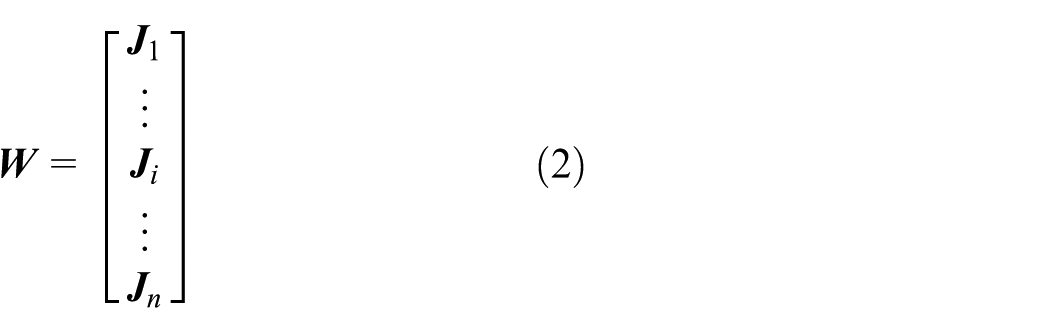
In order to identify the geometrical error parameters Δ
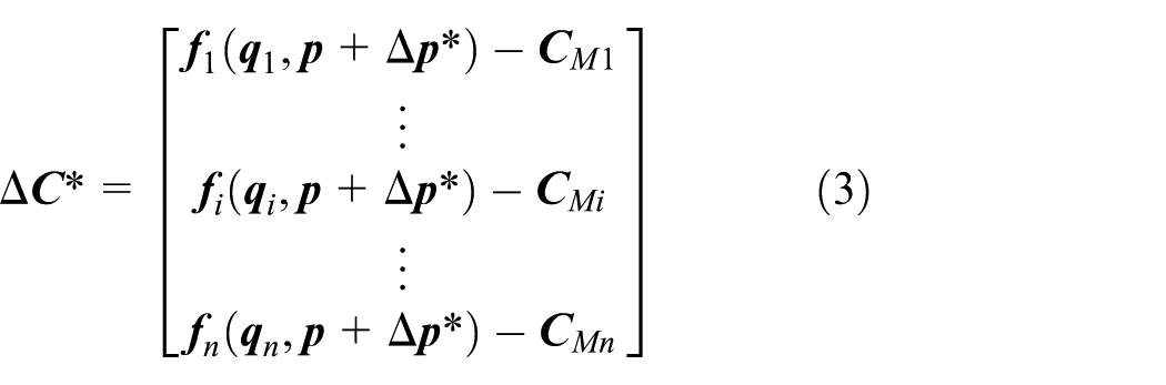
where
At last, based on equations (2) and (3), the parameter identification model can be shown as follows

It should be pointed out that Δ
Equation (4) is a linear equation in which the geometrical error parameters are solved by different algorithms. If the solved Δ

where m represents the iterative number,
It is seen that each iterative step makes the Δ
Analyses of two algorithms (LS and RE) with SVD
LS and RE are the two frequently used algorithms to solve Δ
First, LS is introduced and analyzed. The LS expression to solve geometrical error parameters is written as follows

In order to analyze mathematical property of this algorithm, SVD is employed.

It is a normal SVD format of

Furthermore

Equation (9) reveals that the vector Δ
In order to figure out the linear relation, equation (9) is rewritten as follows

where
In equation (10), it is found that solving Δ

The solving process.
Second, RE is introduced and analyzed. Basically, RE is derived from LS. The RE expression is written as follows
where λn is a vector and called as the RE algorithm parameter. Each element of λn should be bigger than 0.
Equation (11) is rewritten in SVD format

where λi is the element of λn.
In the past investigations, λi is usually replaced by a constant number λ for convenience. This article also adopts this way as follows

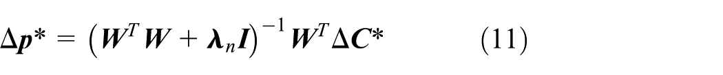
From the above analysis, λ is introduced to modify τi of the solving system. With adjusting λ, namely, changing the solving system, RE can match with the different measuring DOFs. λ needs to be determined before the parameter identification is performed. However, no available formulas can give λ. It is hard to obtain a suitable λ, which just relies on trying different values and always consumes a lot of time.
Analysis of TSVD
LS uses the original solving system with the given j and τi, and RE changes τi to modify the solving system. Obviously, another algorithm to modify j of the solving system can be obtained, which is the TSVD. Before presenting TSVD, a deep investigation on how RE works is given.
From the point of mathematics, τi influences the variance of output solutions in the solving system. If the τi is not changed, the solution has no variance, and the real solution can be obtained. However, when not all motions of the end effector are measured, the real solution will be nonexistent. At this situation, an approximate solution which should approach the real solution is needed. Hence, the variance of solutions should be allowed. The direct way to allow the variance is to modify the singular value τi, as shown in equation (13). The suitable λ is used to overcome the nonlinear ill-conditioning problem, which introduces the variance of solutions and makes the modified solving system approach the original solving system. Since parts of motions of the end effector cannot be measured, the real solution cannot be obtained in fact. The solution of RE approaches the real solution as close as possible by adjusting λ. If λ is too small, RE may be performed like LS that cannot overcome the nonlinear ill-conditioning problem. If λ is too big, RE may destroy the linear relation between the output error parameters and geometrical error parameters (namely, the variance of solutions is allowed too big), which makes the solution of RE be far away from the real solution. Hence, in RE, the key point is to determine λ.
By adjusting τi, an approximate solution solved by RE approaches the real solution. Obviously, another algorithm to modify j also can achieve an approximate solution. From the point of mathematics, the dimension number j of

where

Similarly, the solution of TSVD approaches the real solution as close as possible by adjusting k. If k is too large, TSVD may be performed like LS that cannot overcome the nonlinear ill-conditioning problem. If k is too small, TSVD may make the resolution of solutions too low, which makes the solution of TSVD to not approach the real solution in a small range. The advantage of TSVD is the way to determine its algorithm parameter k, process of which is simple. In the above analysis, k should approach, but should not be equal to the dimension number j of
From the above analysis, the selection of the algorithm parameters (λ and k) and the number of the error parameters affect each other. But in the standard process of kinematic calibration, the number of the error parameters is determined first. After that the parameters (λ and k) should be selected to match with the error parameters. Hence, it is thought that the number of the error parameters affects the selection of the parameters (λ and k).
Parallel manipulators’ description
Two parallel manipulators are described in this section. The one is a 2-DOF parallel manipulator that is applied in a solar tracker. Another one is a 3-DOF parallel manipulator that is used as a parallel module in a 5-axis hybrid machine tool.
Construction of the 2-DOF parallel manipulator and its system modeling
The 2-DOF parallel manipulator is shown in Figure 2. It is composed of a moving platform, a base platform, and three chains. The base platform is fixed, and the moving platform has two rotational motions. The first chain contains a prismatic (P) joint, a universal (U) joint, and a spherical (S) joint. The second chain contains a P joint, a revolute (R) joint, and an S joint. The third chain contains an R joint and a U joint. Among them, these two P joints are actuated. According to the naming rule for a general parallel manipulator, this 2-DOF parallel manipulator is named as RU-PUS-PRS parallel manipulator.

Construction of RU-PUS-PRS parallel manipulator.
A fixed Cartesian reference coordinate system O-XYZ is fixed at the base platform OB1B2. OB1 is perpendicular to OB2. The Z axis is perpendicular to the base platform. The X axis is pointed from B1 to O, and Y axis satisfies the right-hand rule. A moving Cartesian reference coordinate system N-UVW is fixed at the moving platform NA1A2. NA1 is perpendicular to NA2. The W axis is perpendicular to the moving platform. The U axis is pointed from A1 to N, and V axis satisfies the right-hand rule. C1 and C2 locate at U joint of the first chain and R joint of the second chain, respectively. O and N locate at the centers of R joint and U joint of the third chain, respectively. The guide rails, B1C1 and B2C2, are perpendicular to the base platform, respectively. Each P joint moves along the guide rails. Four Cartesian reference coordinate systems, axial directions of which are the same with O-XYZ, locate at B1, B2, C1, and C2, respectively. They are named as B1-XB1YB1ZB1, B2-XB2YB2ZB2, C1-XC1YC1ZC1, and C2-XC2YC2ZC2.
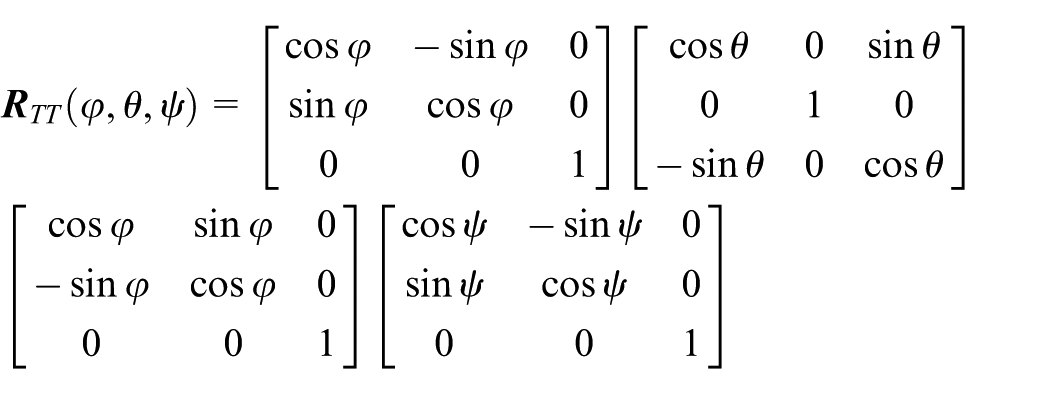
In order to simplify the expression of the rotational matrix, T–T rotational angle in Figure 3 is used to describe the orientation of the moving platform. The rotational matrix is expressed as follows

T–T rotational angle.
The angle ψ is around the normal direction of the moving platform. When the moving platform of a solar tracker follows the sun in the sky, the changing of angle ψ will not affect the tracking accuracy. Hence, angle ψ can be ignored and only two angles are kept in the rotational matrix.
Based on the vector loops OB1C1A1N and OB2C2A2N, the vector loop equations can be written as follows


where
Considering the kinematic constraints of joints and links, the kinematic model can be obtained as follows

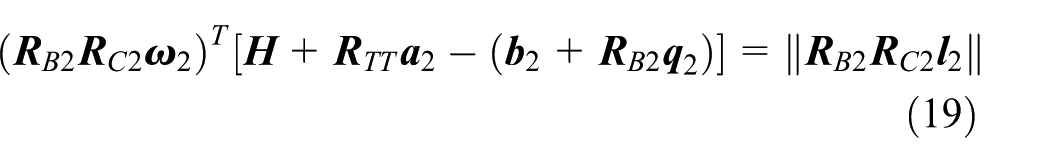
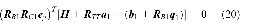


where r represents the length of the link ON,
Based on equations (18)–(23), the error model can be obtained with the linear perturbation method

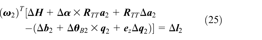


where
In order to make the identification matrix nonsingular, redundant error parameters should be eliminated. By analyzing equations (24)–(29) in scalar expressions, the redundant error parameters which own the same coefficients with others in the error model are eliminated. It is noted that the same analysis is performed in the following parallel manipulator and not repeated again. After the analysis, in total, 25 error parameters can be identified. They are Δa1x, Δa1y, Δa1z, Δb1x, Δb1y, Δ
Construction of the 3-DOF parallel manipulator and its system modeling
The 3-DOF parallel manipulator is shown in Figure 4. It is composed of a moving platform, a base platform, and three supporting chains with the identical kinematic structure. The base platform is fixed, and the moving platform has two rotational motions and one translational motion along Z axis. Each PRS chain contains a P joint, an R joint, and an S joint. Among them, the P joint is actuated. According to the naming rule for a general parallel manipulator, this 3-DOF parallel manipulator is named as 3-PRS parallel manipulator.

Construction of 3-PRS parallel manipulator.
A fixed Cartesian reference coordinate system O-XYZ with Z axis being vertically placed is fixed at the center of the base platform B1B2B3. The X axis is pointed from O to B1, and Y axis satisfies the right-hand rule. A moving Cartesian reference coordinate system N-UVW is fixed at the center of the moving platform A1A2A3. W axis is perpendicular to the moving platform. The U axis is pointed from N to A1, and V axis satisfies the right-hand rule. BiCi on the base platform for i = 1, 2, and 3 represents the guide rail of each chain. The guide rail of each chain is perpendicular to the base platform. Each P joint moves along BiCi. P joint connects the base platform with R joint. R joint connects the P joint with the CiAi link. S joint connects the moving platform with CiAi link. All the joints attached to the base or moving platform are symmetrically distributed at vertices of the equilateral triangles. The Cartesian reference coordinate system Bi-XBiYBiZBi locates at the P joint of each chain. ZBi axis is perpendicular to the base platform. XBi axis is pointed along the direction from O to Bi, and YBi axis satisfies the right-hand rule. The Cartesian reference coordinate system Ci-XCiYCiZCi locates at the R joint of each chain. The directions of ZCi axis and XCi axis are the same with the ones of ZBi axis and XBi axis. YCi axis satisfies the right-hand rule. Bi-XBiYBiZBi and Ci-XCiYCiZCi are used to describe the orientations of P joints and R joints, respectively.
In order to stay the same with RU-PUS-PRS parallel manipulator, T–T rotational angle is also introduced to describe the orientation of the moving platform. Furthermore, the accuracy of the angle ψ is not necessary to assure when the five-axis machine tool machines a part. Hence, angle ψ also can be ignored.
Based on the vector loop OBiCiAiN, the vector loop equations are written as

where
Considering the kinematic constraints of joints and links, the kinematic model can be obtained as

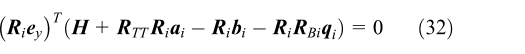
where
Based on equations (31) and (32), the error model can be obtained with the linear perturbation method


where Δ
The redundant error parameters can be eliminated by analyzing equations (33) and (34) in scalar expressions until no error parameters are coupling with others. A total of 11 error parameters on each chain are kept in this error model. They are Δaix, Δaiy, Δaiz, Δbix, Δbiy, Δqi, Δli, ΔθBix, ΔθBiy, ΔθCix, and ΔθCiz. In total, there are 33 error parameters for this parallel manipulator.
Numerical example
In order to show the validity of each algorithm, the parameter identification simulations based on LS, RE, and TSVD are performed, respectively, on the RU-PUS-PRS parallel manipulator and 3-PRS parallel manipulator with 6-DOF measurement. At the same time, the simulations with 5-DOF measurement are also performed, since 6-DOF measurement is hard to achieve in practice, and 5-DOF measurement is enough to guarantee the motion accuracy of these parallel manipulators.
Simulation process of parameter identification
The parameter identification simulations are performed in MATLAB. The detailed process is organized as follows and shown in Figure 5:
Step 1. Initialize the load initial kinematic parameters. Δ
Step 2. Establish the forward kinematic model
Step 3. Select measurement poses. Since the selection of measurement poses can affect the identification result, the distribution of measurement poses keeps in the same in each simulation. The data of measurement poses are given in Appendix 1.
Step 4. Determine the real measurement data. Calculate the real measurement data
Step 5. Obtain the error transfer matrix
Step 6. Generate the identification matrix
Step 7. Identify geometrical error parameters Δ
Step 8. Judge and iterate. If the solved Δ
Step 9. Save the result of geometrical error parameters Δ

Simulation process of parameter identification.
Obtaining the geometrical error parameters is not the end of kinematic calibration. The compensation results still should be simulated for testing these parameter identification results of each algorithm. In general, the motion accuracy of the parallel manipulator should be evaluated by the output error of the moving platform before and after calibration in a given workspace. The original output error before calibration is obtained by
Simulation results
In this section, the parameter identification simulations in different situations are performed based on the above process, and the data are presented in Tables 1–4.
Normal structure parameters of RU-PRS-PUS parallel manipulator.

Normal structure parameters of 3-PRS parallel manipulator.

Output range for evaluating RU-PRS-PUS parallel manipulator.

Output range for evaluating 3-PRS parallel manipulator.

It should be noted that the λ in RE and k in TSVD both greatly affect the identification results. From the above analysis, the k depends on the dimension number of the identification matrix and is determined from big to small. But no investigations give the determination of λ. Considering the mathematical properties, λ is determined according to the smallest singular value of the identification matrix. In the simulations, λ is basically adjusted from the smallest singular value to 1 with the same intervals.
From the analysis in section “Analyses of parameter identification algorithms,” it is known that both λ and k cannot be too big or small. Hence, the curve reflecting the relation curve between the output error and λ or k should be a “V-” or “U”-shaped curve. It can be thought that the best solution can be obtained when a “V-” or “U”-shaped trend emerges. In the following simulations, the best solution of each algorithm is determined by the bottom data of the “V-” or “U”-shaped curve.
The relations between the output error and algorithm parameters (λ and k) in RU-PRS-PUS parallel manipulator with 6-DOF measurement are plotted in Figure 6. The corresponding iteration processes of LS, RE, and TSVD are plotted in Figure 7. The relations between the output error and algorithm parameters (λ and k) in RU-PRS-PUS parallel manipulator with 5-DOF measurement are plotted in Figure 8. Since LS is not suitable with 5-DOF measurement, just the corresponding iteration processes of RE and TSVD are plotted in Figure 9. The corresponding simulation results of 3-PRS parallel manipulator with RE and TSVD are plotted in Figures 10 and 11, respectively. The iteration processes of each algorithm in 3-PRS parallel manipulator are similar with the ones of RU-PRS-PUS parallel manipulator and are not shown again. Since the identified error parameters on each chain are similar with others, the identified error parameters of one chain are organized in Tables 5 and 6. The output errors of each algorithm are organized in Tables 7 and 8. After calibration simulations, the output errors after calibration corresponding to each algorithm parameter are plotted in Figures 6, 8, 10 and 11. In Figures 7 and 9, the horizontal axis represents the iteration number, and the vertical axis represents the value of every error parameter.
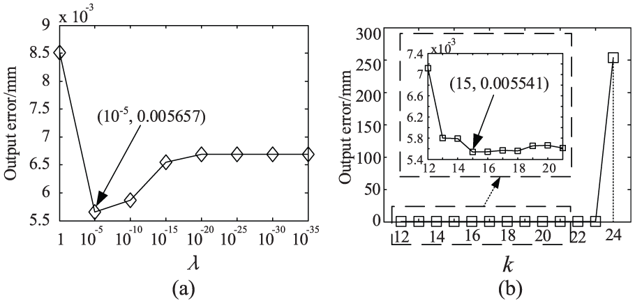
The relations between the output error and algorithm parameters (λ and k) in RU-PRS-PUS parallel manipulator with 6-DOF measurement: (a) RE and (b) TSVD.

The iteration processes of LS, RE, and TSVD in RU-PRS-PUS parallel manipulator with 6-DOF measurement.
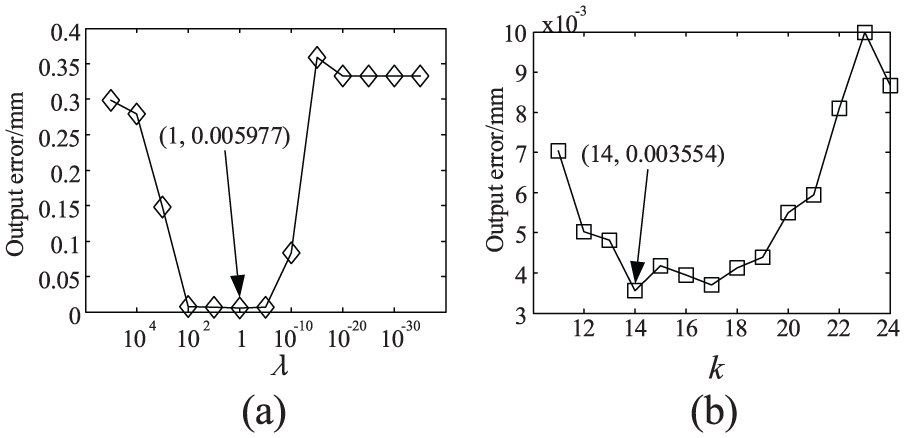
The relations between the output error and algorithm parameters (λ and k) in RU-PRS-PUS parallel manipulator with 5-DOF measurement: (a) RE and (b) TSVD.

The iteration processes of RE and TSVD in RU-PRS-PUS parallel manipulator with 5-DOF measurement.

The relations between the output error and algorithm parameters (λ and k) in 3-PRS parallel manipulator with 6-DOF measurement: (a) RE and (b) TSVD.

The relations between the output error and algorithm parameters (λ and k) in 3-PRS parallel manipulator with 5-DOF measurement: (a) RE and (b) TSVD.
The identified error parameters of one chain in RU-PRS-PUS parallel manipulator.

DOFs: degrees of freedom; LS: least square; RE: ridge estimation; TSVD: truncated singular value decomposition.
The identified error parameters of one chain in 3-PRS parallel manipulator.

DOFs: degrees of freedom; LS: least square; RE: ridge estimation; TSVD: truncated singular value decomposition.
The output errors of RU-PRS-PUS parallel manipulator in different situations.

DOFs: degrees of freedom; LS: least square; RE: ridge estimation; TSVD: truncated singular value decomposition.
The output errors of 3-PRS parallel manipulator in different situations.

DOFs: degrees of freedom; LS: least square; RE: ridge estimation; TSVD: truncated singular value decomposition.
It should be pointed out that the qualitative relationship between the output error and algorithm parameters (λ and k) is suitable for any other parallel manipulators. The quantitative relationship is specific for other parallel manipulators and its key is to obtain the suitable algorithm parameters. For λ, it is needed to find the biggest and smallest values until the solution does not diverge. Then, some suitable values of λ are interpolated between the biggest and smallest values. Compared with choosing λ, k is easy to determine. Since the dimension number of the identification matrix
Discussions
According to the above-mentioned simulation results, several issues about the identified error parameters, LS, RE, and TSVD, are discussed.
In Tables 5 and 6, not all the acceptable identified error parameters approach the real error parameters given in the simulations, no matter which kind of measurement is used or which kind of parallel manipulator is performed. The reason is that with the measurement errors, the real error parameters have not been able to match with the output measurement data. Since the objective of parameter identification is to approach the output measurement data without restraining the changing range of error parameters, some identified error parameters should deviate from the real error parameters in order to fit for the output measurement data. And, different algorithms have different methods to restrain measurement errors, which lead to the different identified error parameters. Furthermore, the accuracy of some local error parameters is affected by the measurement errors. But the accuracy of the global error parameter vectors is effected by the measuring DOF. The 6-DOF measurement can obtain the higher accuracy than the 5-DOF measurement.
In Tables 7 and 8, LS is available with 6-DOF measurement and is totally failed with 5-DOF measurement, the solution of which is emanative. Compared with RE and TSVD, the solution of LS is not the best. But it should be pointed out that LS is still a good algorithm with 6-DOF measurement, since no algorithm parameters are needed to determine, and the solution of LS is usually stable.
In Figures 6(a), 8(a), 10(a), and 11(a), RE is available with both 6-DOF measurement and 5-DOF measurement, no matter which parallel manipulator is simulated. However, the suitable λ in different parallel manipulators is totally different, which ranges from 1 to 10−5. This leads to an obstacle to use RE, since λ is hard to achieve, as this algorithm parameter varies in an unlimited range and is not determined with explicit rules. Furthermore, in practice, this process to change λ will lead to a very tedious and time-consuming routine since every set of identified error parameters with a given λ should be performed on the real parallel manipulator to judge whether the parameter identification result is suitable. It should be noted that λ is chosen in several reasonable values in this article but may be not the best. If it goes on with changing λ in a careful searching, the better identification solution may be obtained in theory. However, it cannot be performed with such a careful searching in practice unless the absolute high-precision identification solution is needed without considering the time cost of searching λ.
In Figures 6(b), 8(b), 10(b), and 11(b), TSVD is available with both 6-DOF measurement and 5-DOF measurements, no matter which parallel manipulator is simulated. In Tables 7 and 8, it is seen that TSVD has the smallest output error values in many situations. Moreover, the algorithm parameter k of TSVD is easy to determine, since k is an integer and its value varies in a limit range with an explicit rule, which means that the error parameters can be identified with a great solution after trying several different k. Another advantage of TSVD is the algorithm convergence. In Figures 7 and 9, the convergence of TSVD is usually faster than the ones of RE and LS.
Furthermore, the method of restraining the measurement error is obtained. The key of this method is to find the best algorithm parameters (λ and k). For λ, it is needed to find the biggest and smallest values until the solution does not diverge. Then, some suitable values of λ are interpolated between the biggest and smallest values. These values can be used for λ in the simulations. Then, the best value of λ among them can be found when a “V-” or “U”-shaped trend like in Figures 6(a), 8(a), 10(a), and 11(a) emerges. Compared with choosing λ, k is easy to find. Since the dimension number of the identification matrix
Conclusion
The parameter identification algorithms of kinematic calibration in parallel manipulators are investigated in this article. By analyzing the identification matrix with SVD, the mathematical properties of LS and RE are investigated, and TSVD is proposed. Parameter identification is to obtain Δ
It should be pointed out that each algorithm has the respective advantages and can be used in the different situations. LS without determining algorithm parameters can be performed in 6-DOF measurement within a short time. RE may obtain the best solution without considering the cost of searching λ. TSVD can obtain a suitable solution with changing k in a limited range.
This article gives the theoretical basis of LS, RE, and TSVD and shows the respective advantages of each algorithm, which are very helpful for the parameter identification in kinematic calibration of parallel manipulators.
Footnotes
Appendix 1
The measurement errors used in 3-PRS parallel manipulator

| Number | X axis (mm) | Y axis (mm) | Z axis (mm) | ϕ angle (rad) | θ angle (rad) | ψ angle (rad) |
|---|---|---|---|---|---|---|
| 1 | 0.006294 | −0.003925 | −0.007118 | 0.000092 | 0.000087 | 0.000162 |
| 2 | −0.002594 | 0.008954 | −0.007379 | −0.000126 | 0.000094 | 0.000154 |
| 3 | −0.009989 | 0.007337 | −0.009301 | 0.000087 | −0.000150 | 0.000055 |
| 4 | −0.001722 | −0.008766 | 0.006013 | −0.000169 | −0.000120 | −0.000077 |
| 5 | −0.009482 | −0.003939 | −0.002417 | −0.000044 | 0.000121 | 0.000020 |
| 6 | 0.008198 | −0.006353 | −0.003175 | −0.000005 | −0.000054 | −0.000115 |
| 7 | −0.007527 | 0.004876 | −0.000682 | 0.000115 | 0.000139 | −0.000018 |
| 8 | −0.005956 | 0.005149 | −0.008085 | 0.000054 | 0.000081 | 0.000125 |
| 9 | −0.003418 | −0.009107 | 0.008304 | −0.000153 | −0.000114 | −0.000090 |
| 10 | 0.002322 | −0.004602 | 0.006181 | −0.000084 | 0.000174 | −0.000092 |
| 11 | −0.005233 | −0.007790 | −0.009851 | 0.000021 | 0.000028 | 0.000001 |
| 12 | −0.005165 | −0.007201 | −0.000967 | −0.000157 | −0.000058 | −0.000136 |
| 13 | 0.009651 | −0.007656 | 0.005592 | 0.000037 | −0.000052 | 0.000024 |
| 14 | −0.001134 | 0.004233 | −0.001695 | −0.000049 | −0.000016 | 0.000151 |
| 15 | −0.001709 | 0.008730 | −0.002535 | 0.000049 | 0.000022 | −0.000040 |
| 16 | 0.004118 | 0.003091 | 0.009072 | 0.000034 | 0.000108 | 0.000078 |
| 17 | 0.000012 | −0.001493 | −0.005028 | 0.000103 | −0.000076 | −0.000143 |
| 18 | −0.002226 | 0.009614 | 0.005378 | −0.000064 | 0.000077 | 0.000141 |
| 19 | 0.000843 | −0.005205 | −0.007866 | 0.000105 | 0.000148 | −0.000045 |
| 20 | −0.002705 | 0.003024 | 0.008812 | −0.000071 | −0.000132 | −0.000100 |
| 21 | −0.005151 | −0.007914 | −0.008827 | −0.000088 | −0.000129 | −0.000022 |
| 22 | −0.002908 | 0.007418 | −0.006329 | 0.000039 | 0.000149 | 0.000002 |
| 23 | −0.002669 | −0.008552 | −0.009570 | −0.000058 | −0.000049 | 0.000091 |
| 24 | −0.009449 | 0.002817 | 0.007943 | −0.000005 | 0.000154 | −0.000006 |
| 25 | 0.002198 | 0.007721 | 0.004058 | −0.000056 | 0.000005 | 0.000084 |
| 26 | −0.004680 | 0.000998 | −0.000997 | −0.000049 | −0.000085 | −0.000101 |
| 27 | 0.000758 | 0.009055 | −0.007891 | −0.000153 | 0.000044 | 0.000049 |
| 28 | 0.005472 | −0.009070 | 0.004182 | 0.000091 | 0.000012 | −0.000111 |
| 29 | −0.007287 | 0.007309 | 0.007403 | −0.000074 | 0.000047 | 0.000065 |
| 30 | −0.000137 | −0.000966 | 0.000159 | 0.000133 | 0.000032 | −0.000014 |
| 31 | 0.004981 | −0.000831 | −0.000710 | 0.000168 | 0.000094 | −0.000165 |
| 32 | −0.001627 | −0.005078 | 0.009168 | 0.000100 | 0.000149 | −0.000165 |
| 33 | −0.004746 | −0.006154 | 0.001240 | −0.000092 | 0.000009 | −0.000049 |
| 34 | 0.007932 | −0.005042 | −0.002239 | −0.000017 | −0.000105 | 0.000112 |
| 35 | −0.009462 | −0.006502 | 0.005346 | 0.000118 | −0.000074 | 0.000168 |
| 36 | 0.008664 | −0.006628 | −0.004280 | −0.000036 | −0.000082 | 0.000151 |
Academic Editor: Jianqiao Ye
Declaration of conflicting interests
The author(s) declared no potential conflicts of interest with respect to the research, authorship, and/or publication of this article.
Funding
The author(s) disclosed receipt of the following financial support for the research, authorship, and/or publication of this article: This work is supported by the National Natural Science Foundation of China (grant nos 51575307 and 51225503), the Science and Technology Major Project-Advanced NC Machine Tools & Basic Manufacturing Equipments (2013ZX04004021 and 2014ZX04002051), and Top-Notch Young Talents Program of China.