A product-of-exponential-based robot calibration method with optimal measurement configurations

Abstract

This article presents a systematic and practical calibration method for an industrial robot to improve its absolute accuracy. The forward kinematics is established based on the global product-of-exponential formula considering some practical constraints. An enhanced partial pose measurement technique is used to construct the linearized error model with only position measurement. All the kinematic parameters are identified via the linear least-squared iteration. The end effector errors are compensated by an inverse Jacobian iteration algorithm in the robot joint space. To suppress the influences of the measurement error, an improved sequential forward floating search algorithm is proposed to select an optimal subset of configurations from a large pool of measured poses based on the D-Optimality. The proposed algorithm is verified via simulations. The calibration method is validated by experiments on an industrial robot, showing that the absolute accuracy of the robot is improved about 10 times under a statistics sense after the calibration.

Introduction

In recent years, industrial robots have been greatly involved in automotive and manufacturing industries, such as handling, assembly, painting, and welding. This attributes to its lower cost, wider workspace, and greater flexibility. However, they are seldom used in high absolute accuracy tasks, such as milling, trimming, and sanding, despite their great potential applications in the aerospace manufacturing industry. ^1,2 Among the factors degrading the accuracy of an industrial robot, geometric errors contribute about 90% of the total error. ³ Geometric errors are mainly caused by the manufacturing tolerance, the assembly misalignment, and the backlash and wear in the transmission chain. Under the influence of geometric errors, the real kinematic parameters of a robot will be slightly different from their nominal values stored in the robot controller, resulting in serious pose error in the end effector (EE).

Robot calibration is identified as a cost-effective way to eliminate or reduce the geometric errors and thus improve the robot absolute accuracy. For example, Tan at al. ⁴ use a vision and pseudoperiodic patterns based measuring system to calibrate a serial micropositioning robot and the positioning accuracy improves by more than 35 times finally. Some other robot calibration-related works can be found in studies by Nubiola and Bonev, Guo et al., Lightcap et al., Motta et al., and Yu et al. ^{5 –9} The vast calibration methods can be roughly grouped into two categories: the modeless calibration methods and the model-based calibration methods. The modeless calibration does not need any kinematic model and directly measures the EE positioning errors at some points and estimates the error on any target point in the whole workspace. ^10,11 These methods are simple and effective, but lead to a huge amount of measurement work to guarantee a considerable accuracy. Therefore, in the literature, the model-based calibration methods have been more researched. This article also adopts this kind of method, thus in the remaining of this research, the word “calibration” is used to represent the model-based calibration for simplicity. Generally, a classical calibration procedure is divided into four steps: modeling, measurement, identification, and implementation. ¹²

The focus of the modeling step is to develop a proper kinematic model to describe the relationship between the robot joint angles and the posture of the EE. The basic requirement for the model is that it should be complete, minimal, and continuous. ¹³ In the last two decades, the modified Denavit–Hartenberg (MDH) model ¹⁴ is mostly used in robot calibration to overcome the discontinuity of the conventional DH model. The complete and parametrically continuous (CPC) model ¹⁵ offers another choice. In general, to meet the requirement of parameter continuity, this kind of models often introduces redundant parameters to describe the homogeneous transformations between adjacent link frames of the robot, leading to a more complex modeling process. In recent years, the product-of-exponential (POE) formula has been more and more used for robot calibration owing to its inherent continuous and complete characteristics and its simple closed-form expression of derivatives of the forward kinematic equations with respect to kinematic parameters. ¹⁶ The POE formula-based robot calibration can be subdivided into the global POE formula-based calibration ^17,18 and the local POE formula-based calibration. ¹⁹ The global one is adopted in this article in terms of simplicity, despite both of the two formulas can efficiently improve the robot absolute accuracy after calibration. Considering the minimality requirement of the model parameters, some researchers proposed some methods to eliminate the redundant POE model parameters. ^{20 –22} Considering the physical constraints of the robot joints, these minimal models mainly add a redundancy elimination step after each iteration in the parameter identification process, and they are reported to have the advantage of a faster convergence in the parameter identification procedure.

The measurement step involves collecting the EE postures (position and orientation) and the joint angle data at some specified points in the robot workspace. The joint angle data can be precisely read in the robot controller from the feedback of the motor encoders and thus do not need any external measurement instruments. While in the robot calibration, the EE posture can be measured by a laser tracker, ⁵ a vision system ²³ or a double ball bar. ²⁴ Sometimes no external measurement instrument is needed if the degrees of freedom (DOFs) of the robot are redundant, which allows self-motion. ²⁵ Among these measurement methods, the laser tracker is mostly used in terms of accuracy and is easy-to-use. In practice, it is usually hard to conduct a full pose measurement, particularly the orientation measurement of the EE. Even if the measurement instrument permitted, the measured full pose errors would suffer a nonhomogeneity problem. ³ Thus, some techniques have been developed to calibrate the robot via only position measurement, ^26,27 and are called the partial pose measurement technique in the study by Wu et al. ³ These methods only use position coordinate information to identify twist parameters, thus, the nonhomogeneity problem is avoided. Another problem in the measurement step is the optimal measurement pose selection of the robot, which means those robot poses that can best suppress the measurement errors should be chosen for the parameter identification. In the literature, many performance criteria have been proposed for the pose selection optimality problem based on the A-Optimality, the E-Optimality, and the D-Optimality in the experiment design theory. ²⁸ Joubair and Bonev ²⁹ conducted a detailed simulation to compare the five different criteria, concluding that the criterion O₁ proposed by Menq ³⁰ based on the D-Optimality outperforms the others most of the time. On the other hand, many algorithms have been developed to solve the optimality problem, such as the genetic algorithm, ³¹ the simulated annealing algorithm, ³² and the most widely used DETMAX algorithm. ^{33 –35} These algorithms all suffer from a local convergence problem.

The essence of the identification procedure is to find a set of kinematic model parameters that best-fit the experimental data. To estimate the best-fitting kinematic parameters, many identification algorithms have been proposed, including the linear least-squared algorithm, the nonlinear least-squared algorithm, and the Kalman filtering estimation technique, and so on. ^12,36 Some numerical issues have been discussed and solved by Hollerbach and Wampler. ³⁷ Among these algorithms, the linear least-squared technique is mostly used in robot calibration owing to its simplicity and unbiased characteristic.

The last step of calibration is the implementation, which concentrates on compensating the geometric errors and improving the final absolute accuracy. Most calibration-related researches have neglected this step. Since there is no access to the internal controller of a robot, the kinematic parameters cannot be modified directly in most commercial industrial robots. An alternative way is to modify the desired posture data in Cartesian space or joint space of the robot in advance. ¹²

In this article, a complete and systematic calibration process is presented for an industrial robot using some state-of-the-art techniques. In this calibration process, the global POE formula is adopted to model the forward kinematics of an industrial robot. An enhanced partial pose measurement technique is used to construct the linear error model considering the base frame errors and the joint twist coordinate errors with only position measurements. The model is solved by a linear least-squared iteration algorithm. The identified kinematic parameters are compensated via an inverse Jacobian iteration method. On the other hand, to suppress the measurement errors, an optimal experiment design process is needed to select a proper set of measurement configurations for parameter identification. Considering the limited workspace of the robot and the measuring range, a number of measurements at points randomly distributed in the robot workspace are conducted in advance, and then an optimal subset of configurations is selected via an improved sequential forward floating search (SFFS) algorithm based on the O₁ criterion. The improved SFFS algorithm we proposed is verified to outperform the most widely used DETMAX algorithm. Finally, some experiments are conducted on an industrial robot, which validate the calibration method.

The remainder of this article is organized as follows. The “Calibration based on the POE” section presents the mathematical model of the calibration procedure. The “Optimal measurement configurations selection” section gives a detailed discussion of the optimal measurement configurations selection method. The “Experiment” section conducts calibration experiments, and the “Conclusion” section concludes the article.

Calibration based on the POE

POE-based forward kinematics for calibration

The forward kinematics of a serial industrial robot with n DOFs based on the POE formula indicates the relationship between the robot base coordinate system { B } and the EE coordinate system { T }, which can be stated as

$g\left(\theta \right)=\prod _{i=1}^n{e}^{{\widehat{\xi }}_i{\theta }_i}{g}_{st}\left(0\right)$

1

In this formula, g_st(0) denotes the initial posture of { T } with respect to { B } with all the joint variables θ = 0, while g(θ) denotes the posture of { T } with a motion $\theta ={\left[{\theta }_1,{\theta }_2,\cdots ,{\theta }_n\right]}^T$ , where θ_i is the ith joint variable. ${\widehat{\xi }}_i\in se\left(3\right)$ represents a twist associated with the ith joint and is expressed in the base frame { B } as

${\widehat{\xi }}_i=\left(\begin{array}{cc}{\widehat{\omega }}_i& v_i\\ 0& 0\end{array}\right)$

2

where $v_i={\left[v_{1i},v_{2i},v_3{}_i\right]}^T\in {ℝ}^3,\text{ and }{\widehat{\omega }}_i\in so\left(3\right)$ is the skew-symmetric matrix of ${\omega }_i,{\omega }_i={\left[{\mathit{\omega }}_{1i},{\mathit{\omega }}_{2i},{\mathit{\omega }}_{3i}\right]}^T\in {ℝ}^3,\text{ and }{\widehat{\omega }}_i$ is given by

${\widehat{\mathbf{\omega }}}_i=\left[\begin{array}{ccc}0& -{\mathit{\omega }}_{3i}& {\mathit{\omega }}_{2i}\\ {\mathit{\omega }}_3{}_i& 0& -{\mathit{\omega }}_{1i}\\ -{\mathit{\omega }}_{2i}& {\mathit{\omega }}_{1i}& 0\end{array}\right]$

3

Generally, ${\xi }_i={\left[{\omega }_i,v_i\right]}^T\in {ℝ}^6$ is called the twist coordinate of the twist ${\widehat{\xi }}_i$ . For a rotation joint, the twist coordinate ξ _i can be expressed as

${\xi }_i=\left[\begin{array}{c}{\omega }_i\\ p_i\times {\omega }_i\end{array}\right]$

4

where ω _i can be physically interpreted as the joint axis direction of the joint i expressed in { B }, and p _i is any point on the same joint axis. More detailed description can be referred to the study by Murray et al. ³⁸ .

As Wu at al. ³⁹ point out, it is necessary to find the coordinate transformation between the robot base frame and the world frame when the robot is required to perform tasks defined in the world frame and offline programming is adopted. Let the measurement coordinate system { M } be the world frame, which is a common situation, then a transformation g₀ should be introduced to express the relation between { M } and { B }. On the other hand, equation (1) needs a full pose measurement of the EE. As stated in the “Introduction” section, it is usually difficult to conduct such a measurement directly. Though some laser tracker manufactures offer the so-called ADM mode (Absolute distance measurement mode, i.e. Measuring the positions of three spherically mounted reflectors (SMRs)), it is less accurate. ⁴⁰ And it will also cause the nonhomogeneity problem. ³ Thus, a forward kinematic model with only position information is needed. In consideration of the two points above, a practical forward kinematic model which is convenient for calibration should be written as

$\begin{array}{l}\left[\begin{array}{c}P\left(\theta \right)\\ 1\end{array}\right]=g_0{\displaystyle \prod _{i=1}^n{e}^{{\widehat{\xi }}_i{\theta }_i}\left[\begin{array}{c}P\left(0\right)\\ 1\end{array}\right]}=e^{{\widehat{\xi }}_0}{\displaystyle \prod _{i=1}^n{e}^{{\widehat{\xi }}_i{\theta }_i}\left[\begin{array}{c}P\left(0\right)\\ 1\end{array}\right]}\end{array}$

5

where g₀ gives the position and orientation of { B } with respect to { M }, and $g_0=e^{{\widehat{\xi }}_0}$ ; also P(0) and P(θ) denote the coordinates of a point on the EE expressed in the base coordinate system { B } with joint variables θ = 0 and θ = θ, respectively. For simplicity, let $g=e^{{\widehat{\xi }}_0}{\displaystyle \prod _{i=1}^n{e}^{{\widehat{\xi }}_i{\theta }_i}},P\left(\theta \right)=P,\text{ and }P\left(0\right)=P_0$ , then equation (5) becomes

$\left[\begin{array}{c}P\\ 1\end{array}\right]=g\left[\begin{array}{c}{P}_0\\ 1\end{array}\right]$

6

Equations (5) and (6) will be used to deduce the linearized error model.

Linearized error model

The linearized error model can be obtained by differentiating equation (6), that is

$\left[\begin{array}{c}dP\\ 0\end{array}\right]=dg\left[\begin{array}{c}{P}_0\\ 1\end{array}\right]+g\left[\begin{array}{c}d{P}_0\\ 0\end{array}\right]=\left(dg{g}^{-1}\right)g\left[\begin{array}{c}{P}_0\\ 1\end{array}\right]+g\left[\begin{array}{c}d{P}_0\\ 0\end{array}\right]$

7

Considering $\left[\begin{array}{c}P\\ 1\end{array}\right]=g\left[\begin{array}{c}{P}_0\\ 1\end{array}\right],\text{ and }dg{g}^{-1}=\left(\frac{\partial g}{\partial {\xi }_0}d{\xi }_0+\frac{\partial g}{\partial \xi }d\xi +\frac{\partial g}{\partial \theta }d\theta \right)g^{-1},\text{ where }\xi =\left[{\xi }_1,{\xi }_2,\cdots ,{\xi }_n\right]\in {ℝ}^{6\times n}$ , the left-hand side of equation (7) represents the errors of a point on the EE expressed in { M } and can be calculated by

$dP=P_a-P_n$

8

where P _a represents the actual coordinate of the point measured by the measurement instrument, and P _n denotes the nominal coordinate of the point calculated by the nominal geometric parameters. The right-hand side of equation (7) represents the geometric errors that cause the EE errors, including the errors in the base frame twist coordinate dξ₀, the errors in the joint twist coordinate dξ, the joint initial offsets dθ, and the initial errors in the specified measurement point dP₀. However, as a matter of fact, the errors dP₀ (sometimes expressed as the EE initial pose error $d{\xi }_{st}$ ), dθ, and dξ₀ cannot be identified simultaneously. In other words, it is impossible to distinguish the EE errors contributed by dP₀, dθ, and dξ₀; thus, they should be separately modeled. ^17,20,21,26 On the other hand, some researchers have developed some methods to identify the exact joint offsets ⁴¹ and the tool-flange transformation ^42,43 ; with these methods, the errors in dθ and dP₀ can be identified solely. Such kinds of identification may be influenced by the robot geometric parameters, which will result in repetitive calibration. Nevertheless, that is out of the scope of this article. Thus, in this article, only dξ and dξ₀ are considered, while dp₀ and dθ related terms are omitted in the subsequent discussion.

Introducing the operator “∨”, which maps a variable ${\widehat{\xi }}_i\in se\left(3\right)\text{ into }{\xi }_i\in {ℝ}^6$ , equation (7) becomes

$\begin{array}{l}\left[\begin{array}{c}dP\\ 0\end{array}\right]=\left(dg{g}^{-1}\right)\left[\begin{array}{c}P\\ 1\end{array}\right]=\left[\begin{array}{c}\left[\begin{array}{cc}-\widehat{P}& I_3\end{array}\right]{\left(dg{g}^{-1}\right)}^{\vee }\\ 0\end{array}\right]\end{array}$

9

that is

$dP=\left[\begin{array}{cc}-\widehat{P}& I_3\end{array}\right]{\left(dg{g}^{-1}\right)}^{\vee }$

10

He et al. ¹⁷ have given the explicit expressions of ${\left(dg{g}^{-1}\right)}^{\vee }$ . A little change is needed in our situation considering the aforementioned conditions. To make the article self-contained, the main computational formulas are listed as follows

${\left(dg{g}^{-1}\right)}^{\vee }=Jdx$

11

and

$\begin{array}{l}J=\left[J_0,J_1,\cdots ,J_n\right]\\ dx={\left[d{\xi }_0,d{\xi }_1,\cdots ,d{\xi }_n\right]}^T\\ J_i=\{\begin{array}{cc}{A}_0& i=0\\ Ad\left({\displaystyle \prod _{k=0}^{i-1}{e}^{{\widehat{\xi }}_k{\theta }_k}}\right)A_i& i=1,\cdots ,n\end{array}\end{array}$

12

where Ad(•) denotes the adjoint transformation of matrix •, and A _i can be calculated by

$\begin{array}{l}{A}_i={\theta }_i{I}_6+\frac{4-{\alpha }_i\text{sin}({\alpha }_i)-4\text{cos}({\alpha }_i)}{2{\Vert {\omega }_i\Vert }^2}{\mathit{\Omega }}_i\\ +\frac{4{\alpha }_i-5\text{ sin}({\alpha }_i)+{\alpha }_i\text{cos}({\alpha }_i)}{2{\Vert {\omega }_i\Vert }^3}{\mathit{\Omega }}_i^2\\ +\frac{2-{\alpha }_i\text{sin}({\alpha }_i)-2\text{ cos}({\alpha }_i)}{2{\Vert {\omega }_i\Vert }^4}{\mathit{\Omega }}_i^3\\ +\frac{2{\alpha }_i-3\text{ sin}({\alpha }_i)+{\alpha }_i\text{cos}({\theta }_i)}{2{\Vert {\omega }_i\Vert }^5}{\mathit{\Omega }}_i^4\end{array}$

13

where ${\mathit{\Omega }}_i=\left[\begin{array}{cc}{\widehat{\omega }}_i& 0\\ {\widehat{v}}_i& {\widehat{\omega }}_i\end{array}\right]\text{ and }{\alpha }_i=\Vert {\omega }_i\Vert {\theta }_i,\left(i=0,1,\cdots ,n,{\theta }_0=1\right)$ .

The above formula with only position measurements is simple and efficient. However, this simplification does not allow the user to identify certain geometric parameters, such as some components of ξ₀. In fact, only three components of ξ₀ can be identified with only one measurement point on the EE. Therefore, the enhanced partial pose measurement method is introduced in the studies of Wu et al. ^3,27 Three points on the EE at each pose of the robot in our situation are measured, and equations (10) and (11) are employed to construct nine equations for each measurement pose. Combining equations (10) to (12) yields

$\left[\begin{array}{c}d{P}_1\\ d{P}_2\\ d{P}_3\end{array}\right]=\left[\begin{array}{ccc}\left[\begin{array}{cc}-{\widehat{P}}_1& I_3\end{array}\right]& & \\ & \left[\begin{array}{cc}-{\widehat{P}}_2& I_3\end{array}\right]& \\ & & \left[\begin{array}{cc}-{\widehat{P}}_3& I_3\end{array}\right]\end{array}\right]Jdx$

14

where P₁, P₂, and P₃ denote the three specified measurement points attached on the EE expressed in { M }. For simplicity, equation (14) is written as

$d{y}_j=K_{j}dx$

15

where j represents the jth measurement pose. Then, the parameter identification problem can be formulated as a linear least-squared problem, which states as

$\underset{{\xi }_0,\xi }{\text{min}}{\displaystyle \sum _{j=1}^m\Vert d{y}_j-K_{j}dx\Vert }{}^2$

16

where m denotes the total measurement times. The geometric parameter error dx can be solved by an iterative method as

$dx={\left(K^{T}K\right)}^{-1}{K}^{T}dy$

17

where $K={\left[K_1,K_2,\cdots ,K_m\right]}^T\text{ and }dy={\left[d{y}_1,d{y}_2,\cdots ,d{y}_m\right]}^T$ . At each step, the model parameters are updated by dx to construct new K and dy, and then a new geometric error dx is calculated. The iteration is terminated when ‖dx‖ becomes sufficiently small. It should be pointed out that the whole process is similar to the one presented in the study by Wu et al. ²⁷ The difference is that in our calibration model, the robot base frame error dξ₀ is included, while this term is not seen in the study by Wu et al. ²⁷ With error term dξ₀, we can not only identify the robot twist parameters but also the transformation between the robot base frame and the measuring frame, which is very important when the robot is required to perform tasks defined in the measuring (world) frame.

Inverse Jacobian iteration-based geometric error compensation

When the identification phase has been finished, the actual kinematic parameters are available. Many calibration-related researches just stop here and evaluate the absolute accuracy by comparing the actually measured EE positions and the ones calculated via the identified geometric parameters. This is not complete and persuasive, because the final absolute accuracy the robot can obtain after calibration is what we really concern. Thus, the position and orientation errors of the EE should be first compensated and then the accuracy can be evaluated. A direct method of compensation is to calculate the inverse kinematic solution of the robot, mapping the desired posture of the EE and the actual kinematic parameters into each joint variable. However, only some simple geometry industrial robots have closed-form inverse kinematic solutions, such as those with three consecutive joint axes intersecting at a common point. Though most industrial robots are designed to have this feature, the condition is usually not satisfied because of imperfect manufacturing and assembly. Therefore, no closed-form inverse kinematic solution is available for the identified actual geometric parameters. To overcome this, an inverse Jacobian iteration algorithm is adopted to compensate the geometric errors.

Assuming the positioning and orientation errors of the EE caused by the nominal kinematic model are small and the desired poses do not fall at or near a robot singular configuration, then the posture error of the EE can be regarded as a differential motion. The robot inverse Jacobian can be used to transform this differential motion into the corresponding joint position changes. The pose error of the EE can be reduced or eliminated via iteratively applying this transformation. The outline of the algorithm is given as follows.

Input: The desired EE pose g _d . The robot nominal kinematic model g = f_n(θ) and the actual kinematic model g = f_a(θ), corresponding to the nominal and the actual kinematic parameters in equation (1), respectively. The solution precision ε.

Output: The desired joint variable θ _d which satisfies $g_d=f_a({\theta }_d)$ .

Initialization: ${\theta }_d^0=f_n^{-1}\left(g_d\right),k=0,\text{ where }{f}_n^{-1}(•)$ represents the inverse kinematic solution.

Step 1: $g_a^{k+1}=f_a\left({\theta }_d^k\right)$ .

Step 2: $d{g}^{k+1}=g_d-g_a^{k+1},\delta =d{g}^{k+1}{g}_d^{-1}$ .

If $\delta =\left[\begin{array}{cccc}{a}_{11}& a_{12}& a_{13}& a_{14}\\ a_{21}& a_{22}& a_{23}& a_{24}\\ a_{31}& a_{32}& a_{33}& a_{34}\\ 0& 0& 0& 0\end{array}\right]$ , then the differential motion of the EE can be written as

$d{x}^{k+1}={\left[\frac{1}{2}\left(a_{32}-a_{23}\right),\frac{1}{2}\left(a_{13}-a_{31}\right),\frac{1}{2}\left(a_{21}-a_{12}\right),a_{14},a_{24},a_{34}\right]}^T$

Step 3: $d{\theta }^{k+1}=J^{-1}d{x}^{k+1},\text{ where }{J}^{-1}$ is the inverse Jacobian matrix of the robot under the nominal kinematic parameters.

Step 4: ${\theta }_d^{k+1}={\theta }_d^k+d{\theta }^{k+1},k=k+1$

Step 5: If $\Vert d{\theta }^k\Vert \le \epsilon$ , terminate the algorithm and output ${\theta }_d={\theta }_d^k$ ; else, go back to step 1.

Given a desired trajectory of the EE, the geometric error of a robot can be compensated in the joint space precisely via the above algorithm. In addition, there is no need to access and modify the internal controller parameters of the robot. More details about calculating the inverse kinematic solution $f_n^{-1}(•)$ and the Jacobian matrix J can be referred to the study by Tsai. ⁴⁴

Optimal measurement configurations selection

Influences of the measurement errors on parameter identification

In the last section, a detailed calibration procedure based on the POE formula is introduced, and the influences of the measurement errors have been ignored. However, the measurement error does have some influences on parameter identification, and this influence can be reduced by just selecting a group of optimal poses for identification based on some optimality criteria.

Assuming that a group of configurations has been selected, and there exists independent normal distributed random errors ${\mathbf{\varsigma }}_i\sim N\left(0,I{\sigma }^2\right)$ for each measurement. Let $\mathbf{\varsigma }={\left[{\varsigma }_1,{\varsigma }_2,\cdots ,{\varsigma }_m\right]}^T$ , and then equation (15) can be written as

$dy+\mathbf{\varsigma }=Kdx$

18

Equation (17) becomes

$d\widehat{x}={\left(K^{T}K\right)}^{-1}{K}^{T}dy+{\left(K^{T}K\right)}^{-1}{K}^T\mathbf{\varsigma }$

19

The identified parameter $d\widehat{x}$ , which is a random vector now, will follow a multivariate normal distribution with the mean vector $E\left(d\widehat{x}\right)=dx$ and the covariance matrix $\text{cov}\left(d\widehat{x}\right)={\sigma }^2{\left(K^{T}K\right)}^{-1}$ . From the joint distribution of the uncertainty parameters, the envelope of $d\widehat{x}$ with probability β can be expressed as

${\left[d\widehat{x}-dx\right]}^T{\left[\text{cov}\left(d\widehat{x}\right)\right]}^{-1}\left[d\widehat{x}-dx\right]={\rho }^2=const$

20

Equation (20) indicates a hyperellipsoid, and the constant size factor ρ is uniquely determined by the significance level β. In geometric terms, the center of the hyperellipsoid is the actual parameter error dx, while the lengths of its principle axes are $\sigma \rho \sqrt{{\lambda }_{{\left(K^{T}K\right)}^{-1}}^i},\text{ where }{\lambda }_{{\left(K^{T}K\right)}^{-1}}^i$ represents the ith eigenvalue of the matrix ${\left(K^{T}K\right)}^{-1}$ . Given the constants ρ and σ, the hyperellipsoid is determined by the matrix K ^T K, which is called the information matrix. The information matrix defines the impact of the measurement errors on the parameter identification process.

Assume that the nominal kinematic parameters are close to the actual ones, and they are used to calculate the information matrix. Then, the two factors determine K ^T K, that is, the measurement times m and the robot configurations selected. Practically, the optimal measurement times are determined by the user’s experience. It is easy to conduct a measurement configuration optimal selection, and this process is called experiment design. Many eigenvalue-based optimizing indices have been proposed for optimal configuration selection, which are based on the A-Optimality, the E-Optimality, and the D-Optimality in the experiment design theory. Among these criteria, the D-Optimality criterion has an advantage of scale independent characteristic ²⁸ and is proved to have a better performance via simulations ²⁹ most of the time. Thus, this criterion is adopted in this article. The D-Optimality means maximizing the determinant of the information matrix

$\underset{\theta }{\text{max}}\left|K^{T}K\right|={\displaystyle \prod _{i=1}^n{\lambda }_{\left(K^{T}K\right)}^i}$

21

where n is the rank of matrix K, and ${\lambda }_{\left(K^{T}K\right)}^i$ is the ith eigenvalue of K ^T K, ${\lambda }_{\left(K^{T}K\right)}^i=\frac{1}{{\lambda }_{{\left(K^{T}K\right)}^{-1}}^i}$ . To be consistent with previous researchers, equation (21) is adjusted to be identical to that in the study by Borm and Meng ³⁰ as

$\underset{\theta }{\text{max}}{O}_1=\frac{\sqrt[n]{{\displaystyle \prod _{i=1}^n{\sigma }_i}}}{m}$

22

where σ_i represents the ith singular value of matrix K, and ${\sigma }_i^2={\lambda }_{\left(K^{T}K\right)}^i$ . The physical meaning of equation (22) is maximizing the inverse of the volume of the hyperellipsoid, that is, minimizing the volume of the hyperellipsoid.

To summarize, the measurement errors have a significant influence on parameter identification, and this influence can be reduced via optimally selecting the measurement configurations of the robot, that is, solving the optimization problem in equation (22).

Improved SFFS for optimal configurations selection

Theoretically, the experiment design process should be conducted in advance, and then the kinematic parameters are identified under a group of optimal robot configurations. However, due to the limited range of the measurement device or obstacles in the robot workspace, some optimal configurations may be impossible to be obtained by the measurement system. This problem motivates us to conduct plenty of measurements in advance and then select a subset of optimal configurations out from the whole set. Then, the complete calibration procedure can be summarized (see Figure 1).

Figure 1.

The complete calibration procedure.

From the above discussion, the optimal measurement configuration selection problem is reduced to a combinatorial problem. That is, given a set of M candidate measurement configurations, select a subset of size m that maximizes the performance measure O₁. This problem is highly complex, and an exhaustive search is computationally prohibitive even for not so large M and m. For example, to select 50 configurations from the whole 100 configurations, one has to calculate more than 10²⁹ combinations via the exhaustive search. In robot calibration experiment design, most researchers search for an optimal pose set with adapted DETMAX algorithm, ^{33 –35,45} which basically replaces the initial subset elements one by one repeatedly. However, all these methods suffer from a local convergence problem. In general, to solve a combinatorial optimality problem, some heuristic or random search algorithms have been developed for other problems, such as the sequential forward/backward algorithm, ⁴⁶ the plus l take away r algorithm, ⁴⁷ and the floating forward/backward search algorithm. ⁴⁸ Among these algorithms, the floating search algorithm has repeatedly been demonstrated to be distinguished in terms of efficiency-effectiveness trade-off. ⁴⁹ Here, the SFFS algorithm is introduced for optimal measurement configuration selection. This algorithm begins with a null configuration set, and for each step, the most significant configuration from the complementary set is included, then the least significant configuration is conditionally eliminated from the selected configuration set, and it continues until the resulting subsets are worse than the previously evaluated ones at that level. Hence, this method is characterized by a dynamically changing number of configurations eliminated at each step until the preset number of configurations m is reached.

The SFFS algorithm cannot avoid a local optimal solution either, despite its efficiency in finding a solution closer to the global one than others. To make this algorithm leave the local convergence and more convenient for solving the experiment design problem, an improved SFFS algorithm is proposed. In the improved version, the following two modifications are proposed based on the randomized search technique. First, the subset is initialized by randomly selecting a least subset of size l. Second, when one search ends, p configurations are randomly deleted from the selected subset and the search process is run iteratively. Every time the best-so-far solution is updated if it is better than the last one. The search process is not stopped until the preset iteration time q is reached. The complete algorithm is depicted in Figure 2. In the figure, “randperm(M,l)” represents generating l distinct random numbers from 1 ∼ M, operator “∪” and “\” denote including or excluding a configuration to or from a configuration subset.

Figure 2.

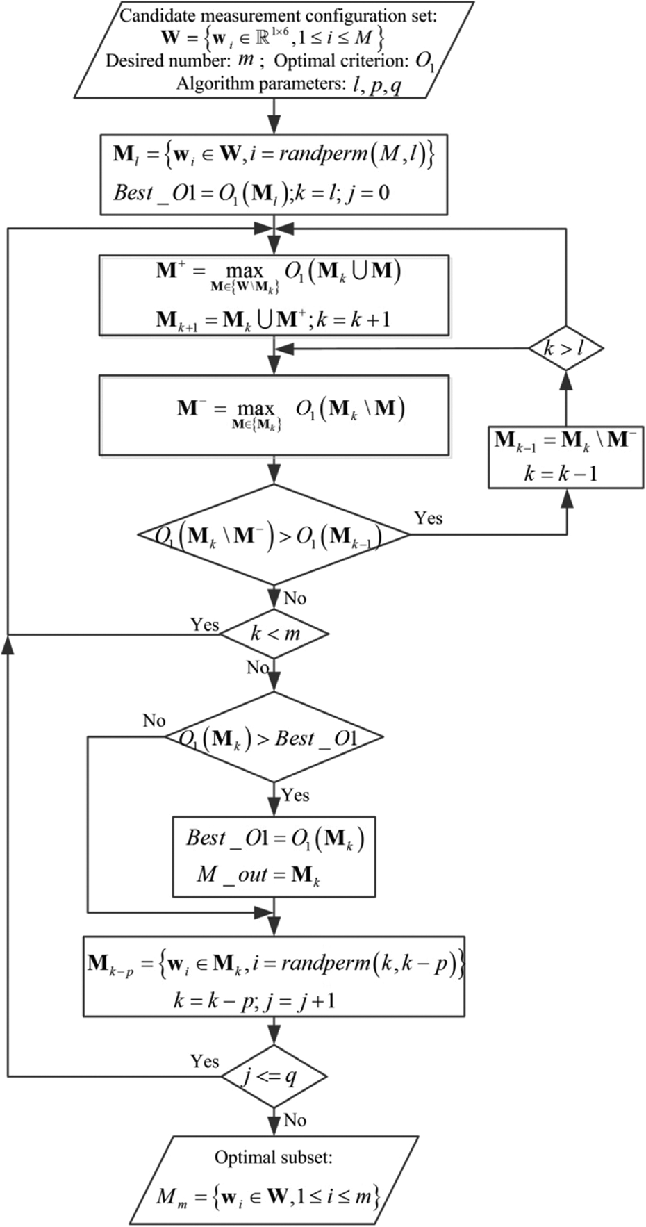
The improved SFFS algorithm. SFFS: sequential forward floating search.

To verify the effectiveness of the proposed algorithm, the following simulation is conducted based on the nominal kinematic parameters of a Motoman MH80 industrial robot. The geometric model of the MH80 industrial robot is shown in Figure 3. Some of the nominal geometric parameters in Figure 3 are listed as follows (the unit is millimeter): $a_1=145,a_2=870,a_3=210,d_5=1025,d_6=175$ , and the corresponding nominal joint twist coordinates based on equation (4) are listed in Table 1. The nominal parameters along with three imaginary SMRs attached on the EE are used to construct equation (14). Sixty configurations are randomly generated as the candidate measurement set, and the goal now is to select 30 optimal poses which maximize the performance measure O₁. For comparison, the values of the performance measure O₁ of the subset selected via random generation, the DETMAX algorithm, the conventional SFFS algorithm, and the improved SFFS algorithm are calculated. The same procedure is executed five times and the results of the calculated O₁ values are listed in Table 2.

Figure 3.

Schematic of the Motoman MH80 industrial robot.

Table 1.

Geometric parameters of MH80.

ξ i	Nominal parameters	Identified parameters
ξ 0	${\left[0,0,0,0,0,0\right]}^T$	${\left[-0.000,-0.001,0.001,1.073,-1.680,-1.185\right]}^T$
ξ 1	${\left[0,0,1,0,0,0\right]}^T$	${\left[0.001,-0.000,1.000,1.873,0.468,0.128\right]}^T$
ξ 2	${\left[0,-1,0,0,0,-145\right]}^T$	${\left[-0.001,-1.001,0.000,0.562,-0.084,-143.648\right]}^T$
ξ 3	${\left[0,-1,0,870,0,-145\right]}^T$	${\left[-0.000,-1.000,0.001,870.853,-1.291,-141.760\right]}^T$
ξ 4	${\left[1,0,0,0,1080,0\right]}^T$	${\left[1.000,0.001,0.001,-0.967,1079.971,0.279\right]}^T$
ξ 5	${\left[0,-1,0,1080,0,-1170\right]}^T$	${\left[0.001,-1.001,0.002,1082.426,-1.432,-1167.510\right]}^T$
ξ 6	${\left[1,0,0,0,1080,0\right]}^T$	${\left[1.000,0.001,0.002,-1.121,1078.568,0.516\right]}^T$

Table 2.

Values of O₁ of the optimal subsets selected via different algorithms.

Algorithm	The ith execution
	1	2	3	4	5
Randomly generated	29.0891	29.1665	29.6886	29.0967	29.4586
DETMAX	32.2801	31.9818	31.9504	31.8213	32.1052
SFFS	32.3389	31.9918	31.9668	31.8519	32.1293
Improved SFFS	32.3389	32.0042	31.9725	31.8588	32.1327

SFFS: sequential forward floating search.

From Table 2, it is obvious that the values of the performance measure O₁ of the subsets selected by the improved SFFS algorithm are a little larger than the others most times, though the gaps are not so significant. That is to say, the measurement configurations selected via the improved SFFS are the global optimum or closer to the global optimum. This owes to the added random process, which is thought to have the ability to improve the result step by step. In addition, by comparing the frequently used DETMAX algorithm and the conventional SFFS algorithm, it can be seen that the latter one has a better performance in selecting optimal configurations.

Experiment

Experiment setup

The calibration system includes a Leica AT901-B laser tracker measurement system, a standard Motoman MH80 industrial robot produced by Yaskawa, an SMR, and three magnetic SMR holders attached on the EE. The laser tracker has a nominal accuracy of ± 10 μm + 5 μm/m and is implemented in the robot workspace which is convenient for measurement. The MH80 robot has a claimed repeated accuracy of ± 0.07 mm while the absolute accuracy is not given in the instruction manual. The whole calibration system is depicted in Figure 4. The measurement coordinate system { M } is established coinciding with the base coordinate system { B } nominally in the Spatial Analyzer software before calibration; thus, the nominal ξ₀ is [0, 0, 0, 0, 0, 0] ^T . After that, the measurements will be conducted. When the robot is moved to a specified measurement pose, the SMR is successively put on the three magnetic holders, and the corresponding 3D position coordinates are measured. The results are all recorded in the software for postprocessing.

Figure 4.

The calibration system.

Calibration validation

The laser tracker repeatability is first verified via the following method. Fix a magnetic holder at some place in the robot workspace within 2 m far from the laser tracker. Then measure the coordinates of the SMR on it from different directions. A total of 30 measurements are conducted. Finally, the repeatability of the laser tracker is calculated based on the ISO 9283 standard. ^50,51 The repeatability of the laser tracker is verified to be ± 12.71 μm, which is consistent with that provided in the user specification. Before the calibration process, the robot is warmed up via actual cyclic motion for an hour from cold start. Then, 100 poses randomly distributed in the robot workspace are measured for parameter identification and verification purposes.

After the measurement step, 50 optimal configurations are selected via the algorithm described in Figure 2. These configurations are thought to be insensitive to the measurement errors and they are used to identify the kinematic parameters. Via the least-squared iteration algorithm, the final kinematic parameters are identified and listed in Table 1. To verify the proposed technique, the center point coordinates of the three measured points at the remaining 50 configurations are calculated using the nominal and the identified parameters, respectively, and they are compared with the measured ones to calculate the error, which we call “predicted error” here, and is represented by the distant between the calculated and the measured position, and the results are shown in Figures 5 and 6. It can be seen from Figures 5 and 6 that the accuracy is improved significantly; the maximum and average predicted errors of the 50 verification configurations are reduced from 5.65 mm and 2.47 mm to 0.60 mm and 0.27 mm. The positioning accuracy predicted by the identified parameters is improved by an order of magnitude.

Figure 5.

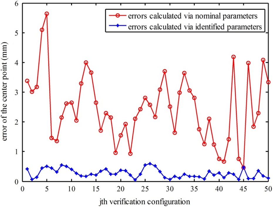
Predicted errors via different parameters.

Figure 6.

Maximum and average errors predicted via different parameters.

To further verify the calibration process, all the 100 EE poses defined by the three measured points are taken as the desired poses. The compensation algorithm presented in the “Inverse Jacobian iteration-based geometric error compensation” section is then used to calculate the correct joint angles for each EE pose employing the identified actual parameters. The robot is moved to the calculated configurations and the position coordinates of the three specified points are measured. For comparison, the robot is also moved to those configurations directly calculated by the inverse kinematics under nominal parameters and the same three points are measured. The errors of the center point of the three measured points at all the 100 configurations are shown in Figures 7 and 8. It can be seen that the compensation algorithm improves the absolute accuracy of the robot greatly, and the maximum and average error are reduced from 6.22 mm and 2.59 mm to 0.65 mm and 0.32 mm, respectively.

Figure 7.

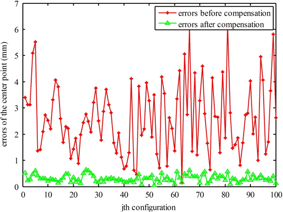
Center point errors before and after compensation.

Figure 8.

Maximum and average errors before and after compensation.

After compensation, the absolute accuracy of the robot should be evaluated. Though the traditional ISO 9283 standard is widely used in industries for robot performance evaluation, ⁵¹ it seems quite unfit to some degree. ^5,40,50 Thus, the following method is used to assess the absolute accuracy of the calibrated robot. Assuming that the positioning error follows a normal distribution, ^3,5 that is, $X\sim N\left(\mu ,{\sigma }^2\right)$ , then the mathematical expectation μ and the variance σ² can be estimated via the expectation $\overline{X}$ and the variance S² of the 100 samples given a confidence level 1 − α, and they satisfy ⁵²

$\begin{array}{l}\mu \in \left(\overline{X}-\frac{S}{\sqrt{n}}{t}_{\frac{\alpha }{2}}\left(n-1\right),\overline{X}+\frac{S}{\sqrt{n}}{t}_{\frac{\alpha }{2}}\left(n-1\right)\right)\\ {\sigma }^2\in \left(\frac{{\displaystyle \sum _{i=1}^n{\left(X_i-\overline{X}\right)}^2}}{{\chi }_{\frac{\alpha }{2}}^2\left(n-1\right)},\frac{{\displaystyle \sum _{i=1}^n{\left(X_i-\overline{X}\right)}^2}}{{\chi }_{1-\frac{\alpha }{2}}^2\left(n-1\right)}\right)\end{array}$

23

where $t_{\frac{\alpha }{2}}\left(n-1\right)\text{ and }{\chi }_{\frac{\alpha }{2}}^2\left(n-1\right)$ represent t− distribution and χ ² distribution, respectively, and X_i is the ith error. In our case, $\overline{X}=0.32$ , S² = 0.02, and set 1 − α = 0.95, we get $\mu \in \left(0.316,0.324\right),{\sigma }^2\in \left(0.015,0.026\right)$ . This can be seen as the final absolute accuracy estimation of the calibrated robot; that is, the average error of the robot after calibration is in the interval (0.316, 0.324) with a probability of 95%.

Conclusion

In this article, a complete and systematic calibration process for an industrial robot is presented. Within the proposed calibration method, only some position measurements are needed in advance, and the subsequent experiment design, parameter identification, and geometric error compensation steps can be completed automatically by a software integrated with the algorithms presented in the article. The overall absolute accuracy of the robot can be improved significantly. The proposed calibration method can be easily extended to any industrial robot. It will pave the way to practical application of the state-of-the-art calibration techniques in industry.

Another contribution of this article is that we have proposed an improved SFFS algorithm based on randomized search technique. With this algorithm, we can easily select an optimal subset from a large pool of measurement configurations for parameter identification; thus, the impacts of measurement noise on the identification accuracy can be reduced. This algorithm is verified to have a better performance than the most frequently used DETMAX algorithm.