
Abstract
Short-term traffic flow prediction is an important part of intelligent transportation systems research and applications. For further improving the accuracy of short-time traffic flow prediction, a novel hybrid prediction model (multivariate phase space reconstruction–combined kernel function-least squares support vector machine) based on multivariate phase space reconstruction and combined kernel function-least squares support vector machine is proposed. The C-C method is used to determine the optimal time delay and the optimal embedding dimension of traffic variables’ (flow, speed, and occupancy) time series for phase space reconstruction. The G-P method is selected to calculate the correlation dimension of attractor which is an important index for judging chaotic characteristics of the traffic variables’ series. The optimal input form of combined kernel function-least squares support vector machine model is determined by multivariate phase space reconstruction, and the model’s parameters are optimized by particle swarm optimization algorithm. Finally, case validation is carried out using the measured data of an expressway in Xiamen, China. The experimental results suggest that the new proposed model yields better predictions compared with similar models (combined kernel function-least squares support vector machine, multivariate phase space reconstruction–generalized kernel function-least squares support vector machine, and phase space reconstruction–combined kernel function-least squares support vector machine), which indicates that the new proposed model exhibits stronger prediction ability and robustness.
Keywords
Introduction
Short-term traffic prediction is one of the most important areas in intelligent transportation system (ITS) research.1–3 A number of ITS applications such as dynamic route guidance (DRG) and urban traffic control (UTC) can benefit from accurate prediction of traffic variables (including but not limited to traffic flow, travel time, traffic speed, and occupancy) for the short-term future (less than 15 min). In reality, for traffic managers, the short-term traffic variables’ prediction information would enable them to apply traffic control management early enough to prevent traffic congestion rather than to deal with the traffic problems after the traffic congestion has already occurred. For travelers, it would enable them to plan their trips in advance and adjust their way at any moment with the dynamic short-term traffic prediction information. Because of its importance, short-term prediction of traffic flow has generated great interest among researchers and a significant number of methods exist in the literature. These existing methods include but not limited to auto-regressive integrated moving average (ARIMA) model, 4 local linear regression model, 5 Kalman filtering model, 6 and nonparametric regression model. 7 Generally, these prediction methods can be categorized as statistical methods, which develop their predictions based on statistical analysis of historical data. One benefit of statistical methods is that they can make very good predictions when the traffic flow varies temporally. However, these methods often assume several restrictive assumptions, such as the normality of residuals, the stationary of the time series, and a predefined model structure, which are seldom satisfied in the case of nonlinear traffic flow. To overcome this problem, numerous studies have used machine learning methods such as support vector machines (SVM)8–10 and artificial neural networks (ANNs)11–13 as alternative predictors. A machine learning method could approximate any degree of complexity of traffic flow without prior knowledge of problem-solving.
With the development of traffic surveillance systems (it is a part of ITS), more and more real-time traffic data, such as traffic flow, speed, and occupancy, become available in every couple of minutes or seconds. Machine learning methods have gained special attention. Compared with the statistical methods, the machine learning methods are more adaptable and suitable to the short-term traffic variables’ prediction field. SVM is a typical machine learning method and can solve the small sample, nonlinearity, high dimension, and local minima problems effectively. However, the SVM algorithm has a relatively complex computation. To solve this problem, the least squares support vector machine (LSSVM) based on SVM was presented by Suykens and Vandewalle 14 in 1999. Its nature is to translate a quadratic programming problem into solving linear equations, consequently accelerating problem-solving and improving computational convergence. Until now, LSSVM has been successfully used in pattern recognition and nonlinear regression estimation problems. In this article, LSSVM is selected as the basic algorithm for short-term traffic flow prediction. At the same time, to obtain the optimal LSSVM model, it is important to choose a kernel function and determine the kernel parameters. If the kernel function and the parameters are not selected correctly, the LSSVM model will not perform well. Therefore, we construct combined kernel function (CKF) and introduce particle swarm optimization (PSO) algorithm 15 to optimize the parameters of LSSVM.
Recent studies have found that the short-term traffic variables’ time series had nonlinear chaotic phenomena.16,17 Chaos is a universal phenomenon of nonlinear dynamic systems. Some sudden and dramatic changes in nonlinear systems may give rise to complex behavior called chaos. A chaotic system, which may appear to be random but is in effect generated by a deterministic model, cannot be examined by standard statistical techniques. 18 A chaotic time series appears stochastic, but it is actually generated by the deterministic system. Chaotic time series prediction has drawn significant attention of researchers over the past few years and some chaotic prediction methods have been developed for short-term traffic variables’ prediction, such as SVM method, 19 Lyapunov exponent method, 20 and local polynomial prediction method, 21 which are based on dynamics reconstruction technique called phase space reconstruction (PSR) and have also achieved some promising results. However, in these methods, scalar traffic variable is mostly used for PSR. Multivariate time series contains more dynamic information than a scalar time series; using available multivariate time series would improve the prediction performance. 22
In this article, a hybrid short-term traffic flow prediction model (multivariate phase space reconstruction (MPSR)–CKF-LSSVM) based on MPSR and CKF-LSSVM is proposed. First, the C-C method 23 is used to choose the optimal time delay and the optimal embedding dimension of the three traffic variables’ (flow, speed, and occupancy) time series for the PSR. Then, the correlation dimension is calculated by G-P method 24 and it is gradually saturated with increasing the embedding dimension, which indicates that the traffic variables’ time series is chaotic. Finally, the optimal input form of the CKF-LSSVM model was determined by MPSR and the parameters of the model are optimized by PSO algorithm.
The remainder of this article is organized as follows. In section “Methodology,” multivariate chaotic time series analysis theory and CKF-LSSVM model are described briefly, and the hybrid traffic flow prediction model MPSR–CKF-LSSVM is introduced. In section “Empirical analysis,” empirical analysis is performed, and the prediction results of several different prediction models are presented and discussed. In section “Discussion and conclusion,” a brief review of this article and the future research are presented.
Methodology
Multivariate chaotic time series analysis
MPSR
For M-dimensional time series:
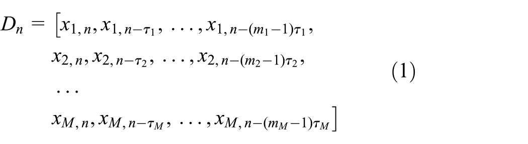
where

The equivalent form of equation (2) can be written as
The remaining problems are how to determine the time delay
In this article,
Determination of time delay and embedding dimension
There are two kinds of views about the selection of these two parameters. One view is that the two parameters are independent and could be determined separately. The methods of calculating delay time include average displacement method,
26
mutual information method,
27
and autocorrelation function method.
28
The methods of calculating embedding dimension include false nearest neighbor method,
29
Cao method,
30
and G-P method.
31
Another view is that the two parameters are interrelated and should be determined simultaneously, such as C-C method.
23
The C-C method can simultaneously estimate the delay time and embedding dimension by applying the correlation integral. Although the C-C method is based on statistical results and has no solid theoretical basis, it is easy to use, requires a small amount of calculation, and also has strong anti-noise capability. Therefore, C-C method is employed to determine delay time
The correlation integral is the following function

where r is the search radius,

The correlation integral is a cumulative distribution function and denotes the probability of distance between any pairs of points in the phase space which is not greater than r. The distance is denoted by the sup-norm of the difference between two vectors.
For


Let t equal or be smaller than 200, the optimal delay time
Correlation dimension
In the chaotic time series analysis, an important step is determining the presence of chaos. One method to determine the presence of chaos uses correlation dimension, 31 which is the most efficient for practical applications. If the correlation dimension is gradually saturated with the increase in the embedding dimension, the system under investigation is considered as chaotic. On the contrary, if the correlation dimension increases without bound with the increase in the embedding dimension, the system under investigation is considered as stochastic.
G-P method proposed by Grassberger and Procaccia
24
is a classical method and frequently used to estimate the correlation dimension. In the G-P method, a double logarithmic plot of the radius and the correlation integral will be an estimate of the correlation dimension. For an m-dimensional phase space, the correlation integral function

where H is the Heaviside step function, with

where

The slope and intercept of the curve between
CKF-LSSVM model
Basic principle of LSSVM
Consider a given training set

subject to

where w is the weight vector,
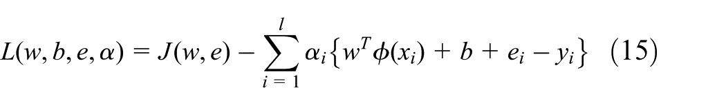
where

By eliminating w and
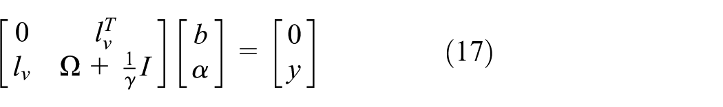
where

where
Sigmoid kernel function

Polynomial kernel function

Gaussian radial basis function (RBF) kernel function

Construction of CKF
The traditional LSSVM model mostly adopts single kernel function to complete the process of feature space mapping, which has achieved good performance in many practical applications. Gaussian RBF kernel function is the most effective one in nonlinear function estimation. 32 However, the single kernel function has great limitations when the sample data contain heterogeneous information. Therefore, this article integrates the Gaussian RBF kernel function (which is a typical local kernel function with strong learning ability and weak generalization ability) and polynomial kernel function (which is a typical global kernel function with strong generalization ability and weak learning ability) to construct a new combination kernel function. The form of combination kernel function is as follows

where
Different kernel functions have different advantages; if the weight coefficient of combination kernel function is inappropriate, the performance of combination kernel function may be lower than single kernel function. Therefore, proper weight coefficient is of great importance for the CKF.
When using the LSSVM method with the CKF, the selection of the CKF parameters
PSO algorithm
The PSO 15 is one of the modern evolutionary computational algorithms and widely used for parameters’ optimization, which is based on the simulation of flocking and swarming behaviors of birds and insects. Compared with other evolutionary computational algorithms, it can efficiently find optimal or near-optimal solutions to the problem under consideration.
In PSO, each particle has its own position and speed, and a potential solution to an optimization problem is represented by the position of one particle. The speed of each particle is updated according to the following two best positions for every iteration. The first one is obtained so far by itself, which can be denoted as


where t is the iteration number, c1 and c2 are the constants called acceleration coefficients, r1 and r1 are the two independent random numbers uniformly distributed in the range of [0, 1], and w is called the inertia factor. The inertia factor w can be set to a constant or a linearly decreasing variable. A nonlinear decreasing w can be determined by
where
MPSR–CKF-LSSVM model
The overall flowchart of MPSR–CKF-LSSVM model is illustrated in Figure 1. The main steps of the short-term traffic flow prediction based on the hybrid MPSR–CKF-LSSVM model are as follows:
Step 1: the C-C method is employed to determine the optimal time delay and the optimal embedding dimension of traffic variables’ (flow, speed, and occupancy) time series for PSR.
Step 2: the G-P method is used to calculate the correlation dimension of traffic variables’ (flow, speed, and occupancy) time series. The correlation dimension is saturated with the increase in embedding dimension, which indicates that these three traffic variables are chaotic.
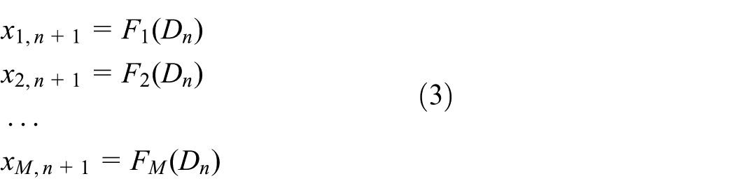
Step 3: the optimal input form of CKF-LSSVM model is determined by PSR of the three traffic variables. Thus, the input and output of CKF-LSSVM model are as follows


Step 4: the parameters of CKF-LSSVM model are optimized by PSO algorithm (4.1) Initialize the particle swarm and CKF-LSSVM model. (4.2) Train CKF-LSSVM model and evaluate the fitness value of all particles. (4.3) Update the particle’s position and velocity according to the position and velocity update formula. (4.4) Judge whether the terminated conditions are met (usually the default calculation accuracy or iterations), and go to Step 4.2 and continue to search if reached; otherwise, continue to Step 4.5. (4.5) Output the optimal parameters of CKF-LSSVM model.

Flowchart of MPSR–CKF-LSSVM model.
Empirical analysis
Data source
The experimental traffic data were obtained from two magnetic coil detectors (No. DC00004965 and No. DC00004966 collected traffic data from east to west and from west to east, respectively) installed at an expressway named Lianqian West Road in Xiamen, China. The traffic data (flow, average speed, and average occupancy) were collected every 5 min in 5 consecutive working days (5 January 2015 to 9 January 2015). Figure 2 gives the traffic data time series from No. DC00004965 detector. Figure 3 shows the three-dimensional scatterplot of traffic flow, speed, and occupancy from No. DC00004965 detector. Traffic data of the first 4 days are used for chaotic time series analysis and training the CKF-LSSVM model. Traffic data of the fifth day are used to test the CKF-LSSVM model.

Traffic data time series from the No. DC00004965 detector: (a) traffic flow, (b) speed, and (c) occupancy.
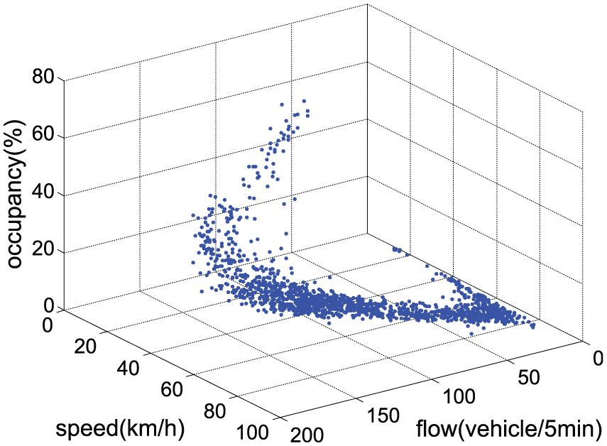
Three-dimensional scatterplot of traffic flow, speed, and occupancy from the No. DC00004965 detector.
In the subsequent section, the data of No. DC00004965 detector are used to illustrate the modeling process in detail, and the two detectors’ data are used to analyze the performance of the model.
Determination of time delay and embedding dimension for MPSR
The C-C method is adopted to calculate the time delay and embedding dimension of the traffic flow, speed, and occupancy time series. Figure 4 gives the curve graph between


Time delay and embedding dimension.

Correlation dimension
Figure 6 shows the relationship of


Relation between correlation dimension
Optimization parameters
The parameters of the CKF-LSSVM model are determined by PSO. To ensure the PSO algorithm efficiency, the mean absolute percentage error as fitness function, and then the fitness function is calculated as follows

where
The traffic data of the first 4 days are used to construct a training set which contains a total of 1025 group input–output mappings. The cross validation method is used to prevent over-fitting and under-fitting. Cross validation is to divide the training data into K groups, then the K − 1 groups are used to train and the other one is adopted to verify the accuracy of the model. It is repeated K times till every group of data is used to verify. The average value of the results from K times verifying is accounted, which is called K-fold cross validation. In this article, fivefold cross validation is used in the training. Model initialization:
The fitness curves are described in Figure 8. The best fitness value is 3.66% and the corresponding optimal parameter combination of CKF-LSSVM model is

Fitness curves of PSO.
Evaluation performance indices
To evaluate the efficiency of the proposed hybrid model, three statistical indices are utilized to measure the prediction accuracy. These indices are the mean absolute error (MAE), mean absolute percent error (MAPE), and equal coefficient (EC). The smaller the values of MAE and MAPE, the more accurate the prediction results. If the value of EC is closer to 1, the prediction result is more accurate. The computing formulas of these indices are as follows

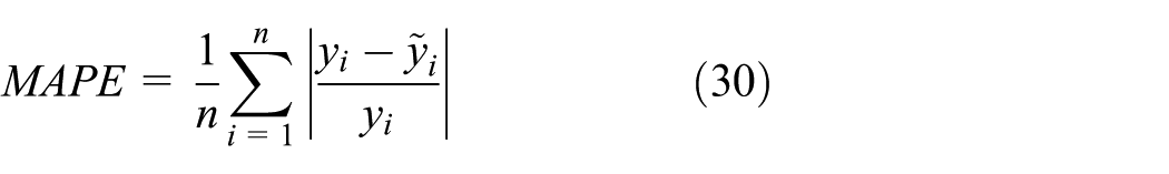

where
Model performance and analysis
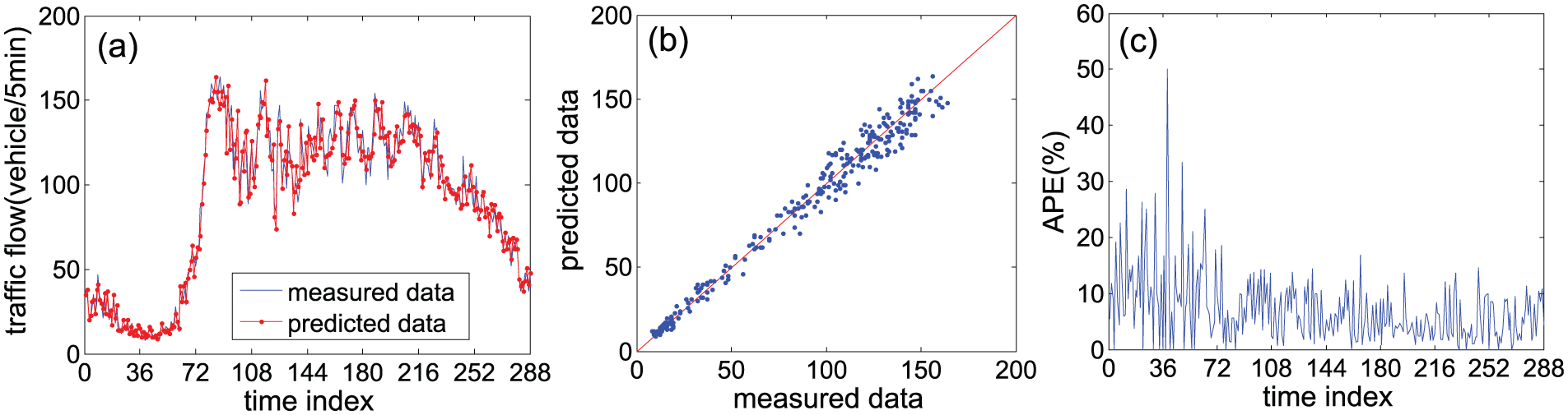
Traffic data of the fifth day are used as test samples to evaluate the performance of the prediction model. In order to illustrate the prediction performance of the proposed method intuitively, Figures 9 and 10 show the prediction results of the proposed model based on No. DC00004965 detector’s data and No. DC00004966 detector’s data, respectively. Figures 9(a) and 10(a) present the curves of prediction data and measured data. The prediction curves are quite close to the measured curves. Figures 9(b) and 10(b) present the scatterplots between the predicted and observed traffic flow data. It is clear that these scatter points distribute near the measured line (the red line) without large deviation. Figures 9(c) and 10(c) show absolute percent error (APE) of the proposed model. The APEs are mostly within 15%. However, the APE from 24 to 48 (correspond to 2:00–4:00) is high, and this is because the actual traffic flow data during that time period are small. Overall, the hybrid MPSR–CKF-LSSVM model achieves good prediction performance, which could meet the needs of short-term traffic flow prediction.
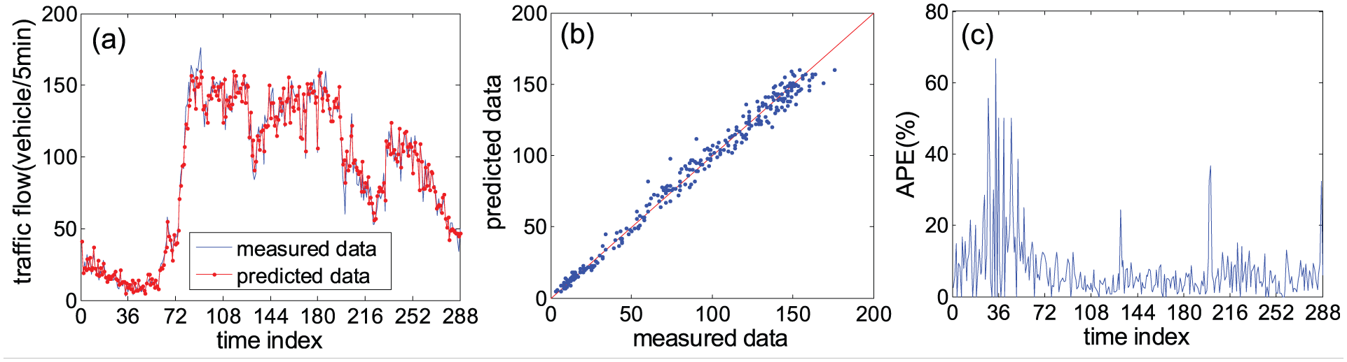
Prediction performance of the proposed method based on No. DC00004965 detector’s data: (a) curves of predicted data and measured data, (b) scatterplot of predicted data and measured data, and (c) absolute percent error of predicted data.
Prediction performance of the proposed method based on No. DC00004966 detector’s data: (a) curves of predicted data and measured data, (b) scatterplot of predicted data and measured data, and (c) absolute percent error of predicted data.
In order to describe the superiority of the proposed model in detail, comparative analysis is carried out. In this article, the comparative models are as follows: the single model (CKF-LSSVM), the hybrid model (MPSR-GKF-LSSVM) based on MPSR and Gaussian RBF kernel function LSSVM, and the hybrid model (PSR–CKF-LSSVM) using PSR and CKF-LSSVM. The input vector of CKF-LSSVM model is the front time series of the predicted value and the dimension of the input vector is the same as MPSR–CKF-LSSVM model. The input vector of MPSR–GKF-LSSVM model is the same as the MPSR–CKF-LSSVM model. While the input vector of PSR–CKF-LSSVM model is determined by a single traffic variable (traffic flow is selected, because the aim of modeling is to predict traffic flow) PSR. Moreover, the parameters of the three comparative models are optimized by PSO.
For the sake of comparison and analysis in terms of macroscopic and microscopic aspects, Figures 11(a) and 12(a) give the microscopic comparative results of different methods based on No. DC00004965 detector’s data and No. DC00004966 detector’s data, respectively. As shown in Figures 11(a) and 12(b), we could see clearly that the prediction results of MPSR–CKF-LSSVM model have the best fitting performance comparing with the other three models, especially when the traffic flow changes greatly (it is clearly shown in Figures 11(b)–(d), and 12(b)). Figure 13(a) and (b) show absolute error (AE) of the four prediction models based on No. DC00004965 detector’s data and No. DC00004966 detector’s data, respectively. We could see clearly that the range of AE based on MPSR–CKF-LSSVM model is minimum, which illustrates the prediction model has better stability. Therefore, the MPSR–CKF-LSSVM model could further improve the accuracy of short-term traffic flow prediction.

(a) Prediction results of different models based on No. DC00004965 detector’s data and (b)–(d) its parts’ specific prediction results.

(a) Prediction results of different models based on No. DC00004966 detector’s data and (b) its parts’ specific prediction results.

Absolute error of different models based on (a) No. DC00004965 detector’s data and (b) No. DC00004966 detector’s data.
The prediction accuracy is shown in Table 2 using three statistical indices (MAE, MAPE, and EC). We could see that the overall improvement of the MPSR–CKF-LSSVM model is obviously comparing to the other three models. More precisely, the MPSR–CKF-LSSVM model has an extra 41.5% improvement over the CKF-LSSVM model, an extra 23.9% improvement over the MPSR–GKF-LSSVM model, and an extra 34.0% improvement over the PSR–CKF-LSSVM model in the aspect of MAE. In the aspect of MAPE, the MPSR–CKF-LSSVM model has an extra 36.4% improvement over the CKF-LSSVM model, an extra 20.0% improvement over the MPSR–GKF-LSSVM model, and an extra 26.2% improvement over the PSR–CKF-LSSVM model. Meanwhile, the MPSR–CKF-LSSVM model is also superior to the other three models in the aspect of EC. Comparison of the results of the MPSR–CKF-LSSVM model and the MPSR–GKF-LSSVM model shows that the performance of CKF-LSSVM is better than Gaussian RBF kernel function LSSVM. Comparison of the results of the MPSR–CKF-LSSVM model, the PSR–CKF-LSSVM model, and the CKF-LSSVM model shows that using MPSR to determine model’s input form can improve the model’s performance effectively. Furthermore, the experimental results also demonstrate that the MPSR–CKF-LSSVM model achieves good prediction performance for both No. DC00004965 detector’s data and No. DC00004966 detector’s data, which proves that MPSR–CKF-LSSVM model has strong generalization ability. Overall, the proposed model is an effective and accurate method for short-time traffic flow prediction, which can provide satisfactory prediction results.
Performance accuracy for different models.

MAE: mean absolute error; MAPE: mean absolute percent error; EC: equal coefficient; MPSR: multivariate phase space reconstruction; GKF: generalized kernel function; LSSVM: least squares support vector machine; CKF: combined kernel function; PSR: phase space reconstruction.
Discussion and conclusion
A new short-term traffic flow prediction model, named MPSR–CKF-LSSVM, is proposed using a combination of MPSR and CKF-LSSVM. The performance of MPSR–CKF-LSSVM model is compared with the MPSR–GKF-LSSVM model, the PSR–CKF-LSSVM model, and the CKF-LSSVM model using the same real-world traffic data. The comparison results show that the MPSR–CKF-LSSVM model can improve the prediction accuracy effectively. Accordingly, a conclusion can be obtained that the short-term traffic variables’ time series shows chaotic characteristic and it is necessary to use PSR (especially MPSR) for improving short-term traffic prediction accuracy.
In order to obtain more general and robust conclusions, traffic data from different roadways require further exploration. And future studies are required to apply the model to other traffic variables’ data sets (such as travel time, traffic speed, and average occupancy; this study chooses the traffic flow as the demonstration). Moreover, it will be interesting to test traffic data set in different time intervals in the model. Other advanced optimization algorithms should be further studied to search for more appropriate parameter combinations for the new proposed model and to obtain more accurate results of short-term traffic flow prediction.
Footnotes
Acknowledgements
Author Ciyun Lin and Zhaosheng Yang are also affiliated with: State Key Laboratory of Automobile Simulation and Control, Jilin University, Changchun, China.
Academic Editor: Nicolas Garcia-Aracil
Declaration of conflicting interests
The author(s) declared no potential conflicts of interest with respect to the research, authorship, and/or publication of this article.
Funding
The author(s) disclosed receipt of the following financial support for the research, authorship, and/or publication of this article: This research is supported by National Key Technology Support Program (Grant No. 2014BAG03B03), and National Natural Science Foundation of China (Grant Nos. 51408257 and 51308248).