Sage Journals: Discover world-class research

Abstract

This article presents a multi-objective discrete group search optimizer for blocking flow shop multi-objective scheduling problem. The algorithm is designed to search the Pareto-optimal solutions minimizing the makespan and total flow time for the flow shop scheduling with blocking constraint. In the proposed algorithm, a diversified initial population is constructed based on the Nawaz–Enscore–Ham heuristic and its variants. Unlike the original group search optimizer in which continuous solution representation is used, the proposed algorithm employs discrete job permutation representation to adapt to the considered scheduling problem. Accordingly, operations of producer, scrounger, and ranger are newly designed. An insertion-based Pareto local search is put forward in producer procedure, a crossover operation is introduced in scrounger procedure, and a local search based on the insert neighborhood is designed in ranger procedure. A bunch of computational experiments and results show that the proposed algorithm is superior to two existing powerful meta-heuristics in terms of both inverted generational distance and set coverage.

Keywords

Meta-heuristics flow shop multi-objective blocking scheduling

Introduction

Scheduling problems play an important role in industrial engineering and operation research and have attracted widespread scientific attention these years. Two common problems which frequently appear in the scheduling literature are the permutation flow shop scheduling problem (PFSP)^1,2 and job shop scheduling problem (JSP).^3–5 The PFSP assumes that there are enough intermediate buffers for jobs between two consecutive machines, whereas the buffers are limited in real production. If there is no buffer for a job and the next machine is busy, then the job has to stay on the incumbent machine and block itself. Assume that the buffer size is zero between any two consecutive machines, a job is easy to block itself and hence the production is greatly delayed. Such a problem is called the blocking flow shop scheduling problem (BFSP). The BFSP extensively exists in all sorts of industrial environments, such as petrochemical process, batch process, plastics molding, and steel manufacture.^6,7

A great deal of research work has been done on the BFSP. It was proved to be non-deterministic polynomial-time (NP)-hard for minimizing makespan for the case of more than two machines.⁸ In 2007, Companys and Mateo⁹ proposed a branch and bound method for makespan minimization in the BFSP, and they solved the problem instances with small sizes. Hybridizing the dynamic programming and branch and bound methods, Bautista et al.¹⁰ presented a bounded dynamic programming method, and the method was effective for small-size instances but powerless to solve instances with large sizes. As regards the heuristic, there were profile fitting (PF),¹¹ Nawaz–Enscore–Ham (NEH),¹² minmax (MM), the hybridization of MM and NEH (MME), and the hybridization of PF and NEH (PFE).¹³ In recent years, meta-heuristics have been an extensively used method for the scheduling field. To minimize the makespan in the BFSP, a genetic algorithm was proposed by Caraffa et al.,¹⁴ and a tabu search was presented by Grabowski and Pempera.¹⁵ Besides, some other algorithms, including the hybrid discrete differential evolution algorithm,¹⁶ the iterated greedy algorithm,¹⁷ and the hybrid harmony search algorithm,¹⁸ were put forward. To minimize the total flow time in BFSP, Deng et al.¹⁹ introduced a hybrid discrete artificial bee colony algorithm which achieved good performance.

The above existing researches are oriented to a single criterion, while multi-objective scheduling problems have gained increasing focus since multiple criteria are usually encountered in real-life scheduling problems. For the multi-objective JSP, Gao et al.²⁰ proposed a Pareto-based grouping discrete harmony search algorithm and a discrete harmony search algorithm.²¹ For the multi-objective PFSP, Yenisey and Yagmahan²² provided an extensive review. Although the multi-objective PFSP is widely studied by many researchers, there are less research reports for the multi-objective optimization in the BFSP. This article considers the minimization of both makespan and total flow time and presents a multi-objective discrete group search optimizer (MDGSO) to search the Pareto-optimal solutions.

Multi-objective BFSP

In BFSP, there are n jobs (job j, j = 1, 2, …, n) and m machines (machine M_i, i = 1, 2, …, m). Each job has to be processed first on machine M₁, then on machine M₂, …, and finally on machine M_m. The processing time of job j on machine M_i is known as p(j, i). The blocking constraint exists in the production process, which means there is no buffer between any two consecutive machines. To be specific, the following assumptions are given: (1) at any time, a machine is able to process at most one job, and a job is able to be processed on at most one machine; (2) no job splitting is allowed; (3) all the jobs and machines are available at time zero; and (4) the set-up time, release time, and transfer time are omitted.

A Gantt chart of BFSP with four jobs and three machines is shown in Figure 1, where the blocking time is marked as shadow rectangles. In Figure 1, the job sequence is 1-2-3-4, which consequently results in the makespan 22 and total flow time 62. It is worth noting that a job sequence different from 1-2-3-4 probably causes the changes of makespan and total flow time, and there is contradiction between these two objectives. 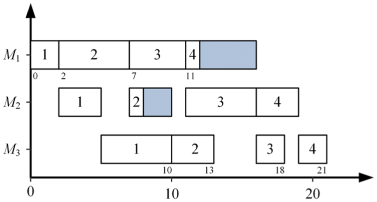Assuming that we have two different schedules $π_{a}$ and $π_{b}$ and the makespan of $π_{a}$ is less than that of $π_{b}$ , there is a possibility that the blocking time in schedule $π_{a}$ is more than that in schedule $π_{b}$ , and hence for some jobs, the completion time in schedule $π_{a}$ is more than that in schedule $π_{b}$ , making the total flow time of schedule $π_{a}$ more than that of schedule $π_{b}$ .

Figure 1.

Gantt chart of a BFSP example.

The minimization criteria in this article are makespan and total flow time. For the considered multi-objective BFSP, the feasible solution is represented as job permutation $π = {π (1), π (2), \dots, π (n)}$ , where $π_{j}$ denotes a job number. Let $d_{π (j), i}$ denote the departure time of job $π (j)$ from machine M_i, then we can compute the departure time first for $π (1)$ , then for $π (2)$ , and so on until $π (n)$ as follows

d_{π (1), 0} = 0

(1)

d_{π (1), i} = d_{π (1), i - 1} + p_{π (1), i}, i = 1, …, m - 1

(2)

d_{π (j), 0} = d_{π (j - 1), 1}, j = 2, \dots, n

(3)

\begin{matrix} d_{π (j), i} = max {d_{π (j), i - 1} + p_{π (j), i}, d_{π (j - 1), i + 1}}, \\ j = 2, \dots, n, i = 1, \dots, m - 1 \end{matrix}

(4)

d_{π (j), m} = d_{π (j), m - 1} + p_{π (j), m}, j = 1, \dots, n

(5)

where $d_{π (j), 0}$ denotes the start time of $π (j)$ on machine M₁.

Let $f_{1} (π)$ and $f_{2} (π)$ denote the objective value of makespan and total flow time of permutation $π$ , respectively, then we have

f_{1} (π) = d_{π (n), m}

(6)

f_{2} (π) = \sum_{j = 1}^{n} d_{π (j), m}

(7)

These two objective values can be computed in O(mn) time. Let $Π$ denote the set of all the job permutations, the multi-objective BFSP is formulated as

Minimize {f_{1} (π), f_{2} (π)} for all π \in Π

(8)

Pareto domination states that solution $π_{a}$ dominates solution $π_{b}$ if and only if $\forall i \in {1, 2}, f_{i} (π_{a}) \leq f_{i} (π_{b})$ and $\exists i \in {1, 2}, f_{i} (π_{a}) < f_{i} (π_{b})$ . Solution $π_{a}$ is optimal in the Pareto sense if there is not any solution $π_{b}$ which dominates $π_{a}$ . Pareto-optimal set is the set containing all Pareto-optimal solutions and Pareto front is the set of all objective values corresponding to the solutions in the Pareto-optimal set.

This article aims to solve the multi-objective problem by Pareto-optimal approach and propose a newly designed algorithm for the considered problem.

MDGSO

The group search optimizer (GSO) was first presented for the continuous function optimization.²³ The population of the GSO consists of three roles: producers, scroungers, and rangers, and each role has its specific updating mechanism. Producers perform producing strategy by simulating the animal scanning mechanism, scroungers perform scrounging strategy by joining resources uncovered by others, and ranger search for the resources by random walks. In each generation, the best member is selected as the producer, and certain individuals in the group are treated as scroungers, while the other individuals are handled as rangers.

Since the scheduling problem is different from the continuous function optimization problem, here individuals in GSO are designed as job permutations $π$ . Besides, the problem considered here is a multi-objective problem, so the mechanisms of producers, scroungers, and rangers need to be newly designed.

Population initialization

In each generation, the proposed MDGSO maintains a population with size ps, which is denoted as PL = {L₁, L₂, …, L_ps}. To get an initial PL with good performance, both the NEH and NEH_WPT²⁴ heuristics are applied. Specifically, we use the NEH heuristic to construct a permutation $π_{NEH}$ for the makespan criterion. Then, the NEH_WPT heuristic is performed to generate a permutation $π_{NEH_WPT}$ for the total flow time criterion. Note that the NEH-WPT was validated as an effective heuristic for the total flow time criterion. The two solutions are added into PL, and the remaining ps-2 initial individuals are generated randomly. Such an initial strategy is able to obtain an initial population with both diversity and quality.

The algorithm also maintains a set of non-dominated solutions, which is denoted as NS = {S₁, S₂, …, S_nb}, where nb is the incumbent size of NS. The set NS is an independent set which stores the non-dominated solutions found by the algorithm so far. After the initialization of PL, the NS is initialized by the non-dominated solutions of PL. Besides, each solution in PL is initially marked as “unsearched.” An example of PL and NS is shown in Figure 2, where ps = 20 and nb = 6.

Figure 2.

Solutions in population and non-dominated set.

Producer procedure

The purpose of producers is to explore the neighborhood region of a relatively better solution. For the multi-objective problem, the relatively better solutions are non-dominated solutions stored in NS. So the producer is designed as follows:

Step 1. If there exists an “unsearched” solution S_k in NS, then let X = S_k, and go to Step 3.

Step 2. Randomly select a solution S_h from NS, and let X = S_h. Apply d insert moves to X and perform an insertion-based Pareto local search (IPLS) on X.

Step 3. Perform IPLS on X. If X is not updated, mark the corresponding S_k in NS with “searched.”

In Step 1 of the above procedure, the solution S_k is selected as follows: if there exists one and only one “unsearched” solution in NS, then the solution is assumed as S_k; if there exists more than one “unsearched” solutions in NS, then a randomly selected one among them is assumed as S_k.

In Step 2 of the above procedure, the insert move means randomly selecting a job from the permutation and inserting it to another position of the permutation. The IPLS searches the insert neighborhood of X in the way that X is updated if and only if a neighbor dominates X. The searching process does not stop until a local optimum is found. The steps of IPLS are as follows:

Step 1. Randomly generate a permutation $π r = {π r_{1}, π r_{2}, \dots, π r_{n}}$ , and let i = 0 and j = 1.

Step 2. Find the position of job $π r_{j}$ in X, insert the job into the other n − 1 positions in X to obtain n − 1 solutions, and find the local non-dominated solution set (denoted as LNS here) of these n − 1 solutions.

Step 3. If there exists an $X' \in LNS$ and $X' ≺ X$ , then let LNS = LNS\X′, $X = X'$ , i = 1; else i = i + 1.

Step 4. Let j = (j + 1) % n, update NS using LNS and mark all the newly added solutions in NS as “unsearched.”

Step 5. If i < n, go to Step 2; else update NS using X and mark all the newly added solutions in NS as “unsearched.”

Note that the producer procedure is applied for one time in each generation, and whenever a solution is newly added in NS, the algorithm does not apply the producing operation on it immediately, just marking it as “unsearched.”

Scrounger procedure

In each generation, all the individuals in the population are either selected as scrounger (with probability p) or ranger (with probability 1 − p). In MDGSO, the scrounger is designed by introducing the crossover operator in genetic algorithm. Specifically, we randomly select a solution in NS and apply partially mapped crossover to it and the current scrounger individual. Then, the current scrounger individual is updated according to the dominance relations of parent and offspring. The steps of scrounger procedure are as follows:

Step 1. Randomly select a solution (denoted by S_k) in NS and perform partially mapped crossover on S_k and the current scrounger individual (denoted by L_i). Denote the obtained offspring as X₁ and X₂.

Step 2. Update NS using X₁ and X₂ and mark all the newly added solutions in NS as “unsearched.”

Step 3. If $L_{i} ≺ X_{1}$ ( $A ≺ B$ means A dominates B) and $L_{i} ≺ X_{2}$ (see Figure 3(a)), then L_i remains unchanged; if $L_{i} ≺ X_{1}$ (or X₂) but L_i does not dominate X₂ (or X₁) (see Figure 3(b)), then L_i is replaced with X₂ (or X₁); if L_i does not dominate X₁ and L_i does not dominate X₂, then two cases exist: if X₁ (or X₂) dominates X₂ (or X₁) (see Figure 3(c)), then L_i is replaced with X₁ (or X₂); else (see Figure 3(d)), L_i is replaced with a randomly selected offspring.

Figure 3.

The dominance relation of offspring solutions (a) L_i dominates both x₁ and x₂, (b) L_i dominates x₁ but not dominates x₂, (c) L_i does not dominates x₁ or x₂ while x₁ dominates x₂, (d) L_i does not dominates x₁ or x₂ while no domination relation exists between x₁ and x₂.

Ranger procedure

In GSO, ranger is designed to perform random search; however, in the proposed MDGSO, the search procedure of ranger is not completely random but based on the solution set NS. For a ranger L_i, first a solution in NS is randomly selected. Then, the insert neighborhood (denoted as Nb(X) for solution X) is searched and a descend direction is selected. The search process iterates until the solution could not be improved in that descend direction. At the end of ranger procedure, the incumbent ranger individual L_i is replaced by the final solution found by the search process. The whole steps are as follows:

Step 1. Randomly select a solution S_k in NS, and let X = S_k.

Step 2. If there exists a solution $X' \in Nb (X)$ , and $f_{1} (X') < f_{1} (X)$ , then go to Step 3; if there exists a solution $X' \in Nb (X)$ , and $f_{2} (X') < f_{2} (X)$ , then go to Step 4; else stop.

Step 3. Nb(X) = Nb(X)\X′, update NS using Nb(X) and mark all the newly added solutions in NS as “unsearched.” $X = X'$ , if there exists a solution $X' \in Nb (X)$ , and $f_{1} (X') < f_{1} (X)$ , then go to Step 3; else go to Step 5.

Step 4. Nb(X) = Nb(X)\X′, update NS using Nb(X) and mark all the newly added solutions in NS as “unsearched.” $X = X'$ , if there exists a solution $X' \in Nb (X)$ , and $f_{2} (X') < f_{2} (X)$ , then go to Step 4; else go to Step 5.

Step 5. Update NS using X. If X is newly added in NS, denote it as “searched.” The incumbent ranger individual L_i is replaced by X.

Procedure of MDGSO

In the proposed MDGSO, the iteration is executed after the initial population PL and non-dominated solution set NS is generated. In each iteration, first the producer procedure is performed, then for each individual in PL, either scrounger procedure (with probability p) or ranger procedure (with probability 1 − p) is performed. There are only three parameters, ps, d, and p, to be determined in MDGSO, and the whole procedure is illustrated in Figure 4.

Figure 4.

The flow chart of MDGSO.

Computational experiments and results

To validate the effectiveness of the proposed MDGSO, the well-known Taillard benchmark set which can be downloaded from the OR library (http://people.brunel.ac.uk/∼mastjjb/jeb/info.html) was used. This article tackled 90 instances, in which job number is from 20 to 100, and machine number is from 5 to 20. It should be noted that all tested algorithms were programmed in C++ language, and a PC with Window 7 operating system, Intel(R) Core(TM) i7-2600 CPU @3.06 GHz and 4 GB RAM was used to execute the algorithms.

Performance measures

There are various performance measures for multi-objective optimization to compare the performance of different algorithms. We use the following two measures:

1. Inverted generational distance (IGD).²⁵ Let P* be a set of reference solutions and A be the non-dominated solution set found by an algorithm. The generalized distance of point x and point y is

d (x, y) = \sqrt{\sum_{i = 1}^{2} {(\frac{f_{i} (x) - f_{i} (y)}{f_{i}^{max} - f_{i}^{min}})}^{2}}

(9)

where $f_{i} (\cdot)$ is the ith objective value, and $f_{i}^{max}$ , $f_{i}^{min}$ are the maximum value and minimum value of the ith objective for P*.

The IGD for A is computed as

IGD (A, P^{*}) = \frac{1}{| P^{*} |} \sum_{y \in P^{*}} min_{x \in A} d (x, y)

(10)

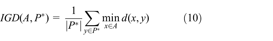
The IGD index reflects the average value of the minimum distance of A and all solutions in P*.

2. Set coverage.²⁶ Let A and B are two non-dominated solutions, the set coverage C(A, B) represents the percentage of solutions in B that are dominated by at least one solution in A, computed as

C (A, B) = \frac{| {x \in B | \exists y \in A : y ≺ x} |}{| B |}

(11)

Computational results

In our computational experiments, the MDGSO was applied to solve each of the 90 instances with 10 replicates. Note that for each instance, we could obtain a solution set for each run. For convenience, all the solution sets of 10 replicates were gathered and a non-dominated solution set A was obtained. Two existing powerful meta-heuristics, non-dominated sorting genetic algorithm (NSGA-II)²⁷ and bi-objective multi-start simulated annealing algorithm (BMSA),²⁸ were adapted for the considered problem here for comparison. For each instance, we obtained the non-dominated solution set for each algorithm and then the performance measures were computed. Note that since the Pareto front for each instance was not known, the reference solution set P* was formed by gathering all the non-dominated solution sets for all tested algorithms. Regarding the parameter calibration for the MDGSO, the bigger the population size ps, the better the results are expected to be. However, a bigger ps value will inevitably cause more computational expense. Parameter d also affects the performance of the proposed algorithm. If it is too big, the solution obtained by d insert moves in producer procedure will possibly lose good characteristics of the original solution. If it is too small, the obtained solution will be possibly not able to escape the original local optimum. As for parameter p which determines the probability that an individual is treated as scrounger, a relatively bigger value is a better choice since the ranger usually uses lower probability in GSO. After some pilot experiments, we found that when the parameters were set as ps = 15, d = 6, and p = 0.8, the algorithm achieved relatively better performance. Thus, in the computational experiments, the above parameter setting was used for the MDGSO while the parameters of the other two algorithms were set as the original papers in the literature. The stopping criterion was set as 30mn ms.

The statistical results are given in Tables 1 and 2, showing IGD values and set coverage values, respectively. In the tables, the results are grouped by instance size for convenience, and bold numbers denote the better values.

Table 1.

The IGD values of the algorithms for instances grouped by different sizes.

Instance size	IGD
Instance size	MDGSO	BMSA	NSGA-II
20 × 5	0.00	0.00	0.01
20 × 10	0.00	0.00	0.00
20 × 20	0.00	0.00	0.00
50 × 5	0.01	0.11	0.25
50 × 10	0.04	0.13	0.28
50 × 20	0.02	0.04	0.14
50 × 5	0.00	1.89	3.31
50 × 10	0.01	0.43	1.12
50 × 20	0.02	0.32	0.87
Average	0.01	0.33	0.67

IGD: inverted generational distance; MDGSO: multi-objective discrete group search optimizer; BMSA: bi-objective multi-start simulated annealing algorithm; NSGA: non-dominated sorting genetic algorithm.

Table 2.

The set coverage values of the algorithms for instances grouped by different sizes.

Instance size	MDGSO (A) vs BMSA (B)		MDGSO (A) vs NSGA-II (C)
Instance size	C(A, B)	C(B, A)	C(A, C)	C(C, A)
20 × 5	0.01	0.00	0.03	0.00
20 × 10	0.01	0.00	0.01	0.00
20 × 20	0.01	0.00	0.02	0.00
50 × 5	0.82	0.13	0.98	0.00
50 × 10	0.50	0.40	0.81	0.18
50 × 20	0.53	0.41	0.93	0.03
50 × 5	0.96	0.01	1.00	0.00
50 × 10	0.88	0.08	1.00	0.00
50 × 20	0.84	0.08	1.00	0.00
Average	0.51	0.12	0.64	0.02

MDGSO: multi-objective discrete group search optimizer; BMSA: bi-objective multi-start simulated annealing algorithm; NSGA: non-dominated sorting genetic algorithm.

From Table 1, we can see that for the instances with 20 jobs, the differences between the MDGSO and the other two algorithms are not significant, which is probably because of the simplicity of the small-size instances. However, for the instances with 50 and 100 jobs, the IGD values of the MDGSO are clearly greater than the other two algorithms, which indicates the superiority of the MDGSO. We note that for some groups, the IGD values of the MDGSO are nearly zero, which means that the solution sets obtained by the MDGSO are very close to the reference solution sets. Table 1 also indicates the superiority of the BMSA over the NSGA-II.

Table 2 shows the differences of the algorithms’ performances in another facet. For the comparison between the MDGSO and the BMSA, the C(A, B) value is greater while the C(B, A) value is smaller, which indicates that the MDGSO is superior to the BMSA. Similarly, the values in the other two columns validate the superiority of the MDGSO over the NSGA-II.

To show the differences among the algorithms more clearly, we draw the non-dominated solution set of each algorithm for instance Ta36 and Ta86 in Figures 5 and 6, respectively. Note that the non-dominated solution set of each algorithm is formed by the results of 10 replicates. It is seen from these two figures that the non-dominated solutions found by the MDGSO have better diversity as well as better quality than those found by any of the other algorithms. As an example, the Gantt chart of a non-dominated solution for instance Ta01 is shown in Figure 7, where the makespan is 1380 and the total flow time is 15,042.

Figure 5.

The non-dominated solutions obtained by the three algorithms for Ta36.

Figure 6.

The non-dominated solutions obtained by the three algorithms for Ta86.

Figure 7.

Gantt chart of a non-dominated solution for instance Ta01.

Conclusion

This article has presented an MDGSO for the multi-objective optimization in blocking flow shop scheduling. A population initialization method based on NEH heuristic and its variants has been designed to generate diversified solutions. Besides, we have designed the strategies of producers, scroungers, and rangers by hybridizing some local search methods, and we have conducted a multitude of experiments minimizing both the makespan and total flow time objectives in blocking flow shop scheduling. The computational results have shown that the proposed algorithm is superior to both the NSGA and BMSA in terms of IGD and set coverage. In future, we will focus on adapting the discrete GSO to other complex scheduling problems, such as the no-wait job shop problem, the flexible flow shop problem, and stochastic scheduling problem.

Footnotes

Academic Editor: Xichun Luo

Declaration of conflicting interests

The author(s) declared no potential conflicts of interest with respect to the research, authorship, and/or publication of this article.

Funding

The author(s) disclosed receipt of the following financial support for the research, authorship, and/or publication of this article: The authors appreciate the support of National Natural Science Foundation of China (Grant No. 61403180), the Project for Introducing Talents of Ludong University (LY2013005), National Natural Science Foundation of China (Grant No. 51407088), and Promotive Research Fund for Excellent Young and Middle-aged Scientists of Shandong Province (Grant No. BS2015DX018).

References

Garey

Johnson

Sethi

The complexity of flowshop and jobshop scheduling. Math Oper Res 1976; 1: 117–129.

Ruiz

Stutzle

A simple and effective iterated greedy algorithm for the permutation flowshop scheduling problem. Eur J Oper Res 2007; 177: 2033–2049.

Gao

KZ.

Effective ensembles of heuristics for scheduling flexible job shop problem with new job insertion. Comput Ind Eng 2015; 90: 107–117.

Gao

Suganthan

Chua

. A two-stage artificial bee colony algorithm scheduling flexible job-shop scheduling problem with new job insertion. Expert Syst Appl 2015; 42: 7652–7663.

Gao

Suganthan

Pan

. An effective discrete harmony search algorithm for flexible job shop scheduling problem with fuzzy processing time. Int J Prod Res 2015; 53: 5896–5911.

Martinez

Peres

Gueret

. Complexity of flowshop scheduling problems with a new blocking constraint. Eur J Oper Res 2006; 169: 855–864.

Gong

Tang

Duin

CW.

A two-stage flow shop scheduling problem on a batching machine and a discrete machine with blocking and shared setup times. Comput Oper Res 2010; 37: 960–969.

Hall

Sriskandarajah

A survey of machine scheduling problems with blocking and no-wait in process. Oper Res 1996; 44: 510–525.

Companys

Mateo

Different behaviour of a double branch-and-bound algorithm on Fm/prmu/C_max and Fm/block/C_max problems. Comput Oper Res 2007; 34: 938–953.

10.

Bautista

Cano

Companys

. Solving the Fm/block/Cmax problem using bounded dynamic programming. Eng Appl Artif Intel 2012; 25: 1235–1245.

11.

McCormick

Pinedo

Shenker

. Sequencing in an assembly line with blocking to minimize cycle time. Oper Res 1989; 37: 925–936.

12.

Leisten

Flowshop sequencing problems with limited buffer storage. Int J Prod Res 1990; 28: 2085–2100.

13.

Ronconi

DP.

A note on constructive heuristics for the flowshop problem with blocking. Int J Prod Econ 2004; 87: 39–48.

14.

Caraffa

Ianes

Bagchi

. Minimizing makespan in a blocking flowshop using genetic algorithms. Int J Prod Econ 2001; 70: 101–115.

15.

Grabowski

Pempera

The permutation flowshop problem with blocking: a tabu search approach. Omega 2007; 35: 302–311.

16.

Wang

Pan

Suganthan

. A novel hybrid discrete differential evolution algorithm for blocking flow shop scheduling problems. Comput Oper Res 2010; 37: 509–520.

17.

Ribas

Companys

Tort-Martorell

An iterated greedy algorithm for the flowshop scheduling problem with blocking. Omega 2011; 39: 293–301.

18.

Wang

Pan

Tasgetiren

MF.

A hybrid harmony search algorithm for the blocking permutation flow shop scheduling problem. Comput Ind Eng 2011; 61: 76–83.

19.

Deng

A discrete artificial bee colony algorithm for minimizing the total flow time in the blocking flow shop scheduling. Chinese J Chem Eng 2012; 20: 1067–1073.

20.

Gao

Suganthan

Pan

. Pareto-based grouping discrete harmony search algorithm for multi-objective flexible job shop scheduling. Inform Sci 2014; 289: 76–90.

21.

Gao

Suganthan

Pan

. Discrete harmony search algorithm for flexible job shop scheduling problem with multiple objectives. J Intell Manuf 2016; 27: 363–374.

22.

Yenisey

Yagmahan

Multi-objective permutation flow shop scheduling problem: literature review, classification and current trends. Omega 2014; 45: 119–135.

23.

Saunders

JR.

A novel group search optimizer inspired by animal behavioral ecology. In: IEEE international conference on evolutionary computation (CEC’2006), Vancouver, BC, Canada, 16–21 July 2006, pp.1272–1278. New York: IEEE.

24.

Wang

Pan

Tasgetiren

MF.

Minimizing the total flow time in a flow shop with blocking by using hybrid harmony search algorithms. Expert Syst Appl 2010; 37: 7929–7936.

25.

Coello

Cortés

Solving multiobjective optimization problems using an artificial immune system. Genet Program Evol M 2005; 6: 163–190.

26.

Zitzler

Deb

Thiele

Comparison of multiobjective evolutionary algorithms: empirical results. Evol Comput 2000; 8: 173–195.

27.

Deb

Pratap

Agarwal

. A fast and elitist multiobjective genetic algorithm: NSGA-II. IEEE T Evolut Comput 2002; 6: 182–197.

28.

Lin

Ying

KC.

Minimizing makespan and total flowtime in permutation flowshops by a bi-objective multi-start simulated-annealing algorithm. Comput Oper Res 2013; 40: 1625–1647.

A discrete group search optimizer for blocking flow shop multi-objective scheduling

Abstract

Keywords

Introduction

Multi-objective BFSP

MDGSO

Population initialization

Producer procedure

Scrounger procedure

Ranger procedure

Procedure of MDGSO

Computational experiments and results

Performance measures

Computational results

Conclusion

Footnotes

Declaration of conflicting interests

Funding

References