Sage Journals: Discover world-class research

Abstract

In this article, a modification of multi-objective differential evolution based on simulated annealing is proposed to solve a general tri-objective non-permutation flow shop problem. The flow shop system considers the release dates, machine breakdowns, past-sequence-dependent setup times and learning effect for all the jobs. The algorithm proposed to tackle such a model combines the robustness of differential evolution with the rapid convergence and conditional diversification of simulated annealing. For small and medium low-sized problems, the solutions found by the proposed algorithm are compared with the exact solutions, achieved by augmented ε-constraint method. Due to the high complexity of the model, for medium high and large-sized problems, the algorithm is tested against the imperialist competitive algorithm and the multi-objective differential evolution scheduling. Comparisons of the results show a good balance between intensification and diversification in the proposed algorithm.

Keywords

Differential evolution simulated annealing multi-objective scheduling non-permutation flow shop

Introduction

Flow shops are among the most attractive systems in scheduling. However, despite the progressive development of general flow shop models, there is still a noticeable gap between theory and practice.^1,2 Thus, in this article, the following assumptions are considered. First, the truncated version of Dejong’s learning effect³ with operator’s prior experience considerations is added to the model. Learning effect in scheduling refers to the reduction in processing times due to the continuous improvement in the production performance. In other words, as the operator gains more skills, more shortcuts are found and the job is done in a shorter span of time. Moreover, the model considers the past-sequence-dependent (psd) setup times which is usually found in industries such as textile, metallurgical, printed circuit board and automobile manufacturing.⁴ This type of setup time relates the setup time of the current job under schedule to the sum of processing times of the jobs prior to it. The problem under study is a non-permutation flow shop system where the permutation of jobs on the machines is not necessarily the same. Hence, for n jobs and m machines, the solution space of a non-permutation flow shop has $(n!)^{m}$ possible solutions instead of $n!$ alternatives of its permutation counterpart. In reality, machines can be unavailable due to the changes in shifts, periodical maintenances or breakdowns. Thus, predetermined machine availability constraints are also considered.⁵ Moreover, most models in the literature are considered with a single objective despite the fact that real-world problems are multi-objective by nature.^6,7 Considering several objectives in flow shop systems increases the complexity of an already NP-hard (i.e. non-deterministic polynomial-time hard) problem. As a result, most proposed solution techniques are practical up to a limited number of jobs or/and machines.³ Recently, meta-heuristics are proposed as alternative solution techniques.^8,9 Differential evolution (DE) is a new meta-heuristic, famous for its robustness and fast convergence in continuous space.¹⁰ However, in discrete problems such as scheduling flow shop systems, DE can get trapped in the local valley, which arises the need for a diversification mechanism. Simulated annealing¹¹ (SA) has been used to solve scheduling problems for many years. The logic behind SA can be used to find suitable and diverse solutions in flow shops. Inspired by these observations, a hybrid DE is proposed to tackle a tri-objective non-permutation general flow shop problem. The objectives under study are the maximum completion time of all jobs (i.e. the makespan), the sum of flow times and the maximum tardiness of all jobs. The rest of this article is organized as follows. In section “Brief introduction on multi-objective problems,” a brief introduction is given on multi-objective problems. In section “Mathematical formulation,” the system under study is presented and the proposed model of such a system is examined in details. In section “The proposed algorithm,” the proposed hybrid algorithm is explained. Section “Computational experiments” includes discussions on the comparison test results of the proposed algorithm. Finally, this article is concluded in section “Conclusion.” Note that the notation described in each section has the intended meaning in its own section and bears no relevance to the other parts of the article.

Brief introduction on multi-objective problems

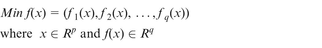
The goal in a general multi-objective minimization problem is to find a set of Pareto optimal solutions within a feasible region which minimizes a vector of objective functions. The objectives are usually unrelated or in conflict with each other. Such a problem with q objectives and p decision variables has the following form

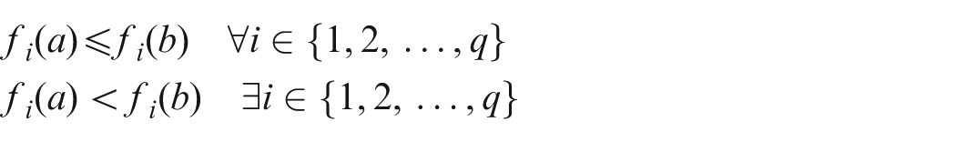
\begin{array}{l} M i n f (x) = (f_{1} (x), f_{2} (x), \dots, f_{q} (x)) \\ w h e r e x \in R^{p} and f (x) \in R^{q} \end{array}

The Pareto optimal solutions (i.e. the set of non-dominated points) are the solutions that cannot be improved in one objective function without deteriorating their performance in at least one of the rest.¹² The concept of domination for solutions $a, b$ can be defined as follows. Here, solution a dominates solution b if and only if

\begin{array}{l} f_{i} (a) ⩽ f_{i} (b) \forall i \in {1, 2, \dots, q} \\ f_{i} (a) < f_{i} (b) \exists i \in {1, 2, \dots, q} \end{array}

Mathematical formulation

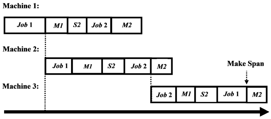
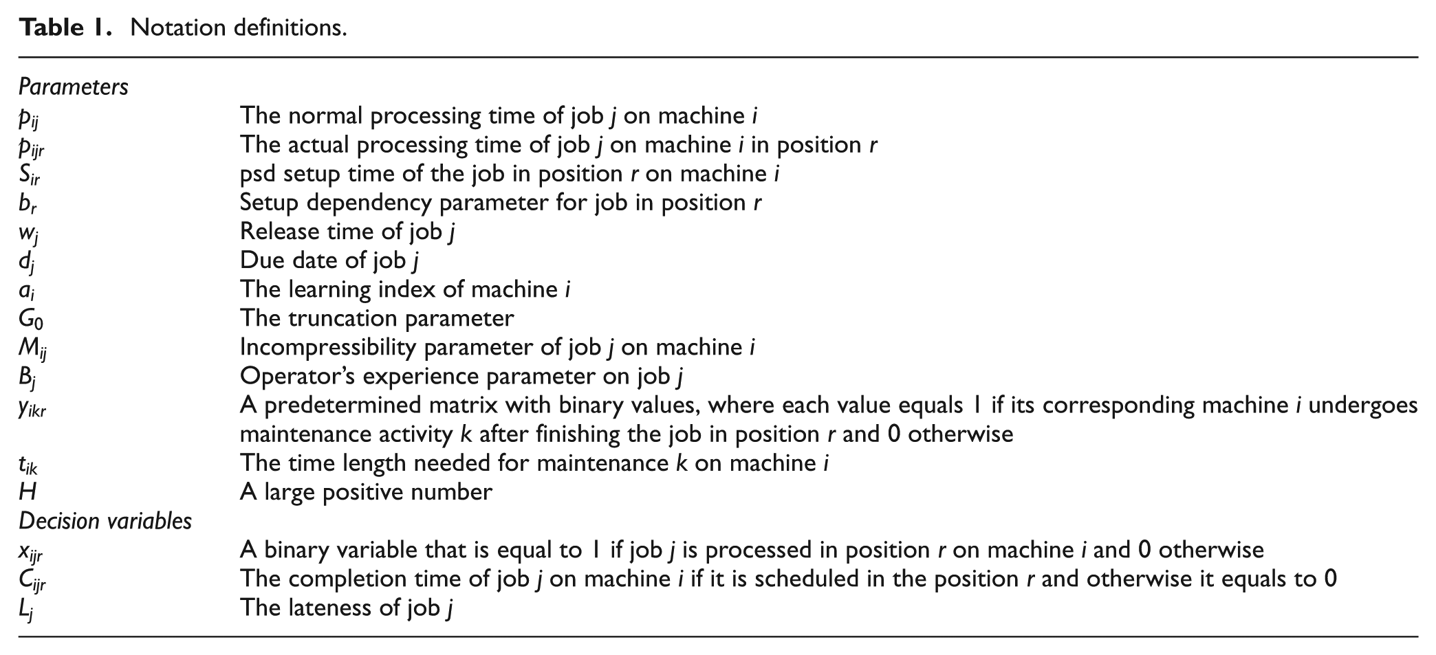
The current model is adapted from the authors’ latest research⁵ but with a modified learning effect. In addition to the learning effect, the model considers separate setup times, maintenance times, release times and due dates. Here, the flow shop problem for m machines, n jobs and K maintenance activities is formulated where all the jobs go through all the machines one by one and are subject to predetermined maintenances. A diagram of such a problem is illustrated in Figure 1 where two jobs on three machines are scheduled. In Figure 1, M1 and M2 are the first and second maintenance activities, respectively. Similarly, S2 refers to the second setup time. Note that for a psd setup time, S1 equals to zero for the first job on each machine and thus it is omitted. The sequences of jobs on different machines are not necessarily the same. For instance, the sequences of jobs on first and second machines are Job1-Job2 but this sequence changes to Job2-Job1 on the third machine. The makespan would be the completion time of the last job on the last machine. Note that a maintenance activity after the last job on each machine does not affect the makespan. First the parameters and decision variables, used in the model, are defined in Table 1. Then, the model is formulated in equations (1)–(8). Here, i, j, r and k are the machine, job, position and the maintenance activity indices, respectively.

Figure 1.

An overview of the system.

Table 1.

Notation definitions.

Parameters
$p_{ij}$	The normal processing time of job j on machine i
$p_{ijr}$	The actual processing time of job j on machine i in position r
$S_{ir}$	psd setup time of the job in position r on machine i
$b_{r}$	Setup dependency parameter for job in position r
$w_{j}$	Release time of job j
$d_{j}$	Due date of job j
$a_{i}$	The learning index of machine i
$G_{0}$	The truncation parameter
$M_{ij}$	Incompressibility parameter of job j on machine i
$B_{j}$	Operator’s experience parameter on job j
$y_{ikr}$	A predetermined matrix with binary values, where each value equals 1 if its corresponding machine i undergoes maintenance activity k after finishing the job in position r and 0 otherwise
$t_{ik}$	The time length needed for maintenance k on machine i
H	A large positive number
Decision variables
$x_{ijr}$	A binary variable that is equal to 1 if job j is processed in position r on machine i and 0 otherwise
$C_{ijr}$	The completion time of job j on machine i if it is scheduled in the position r and otherwise it equals to 0
$L_{j}$	The lateness of job j

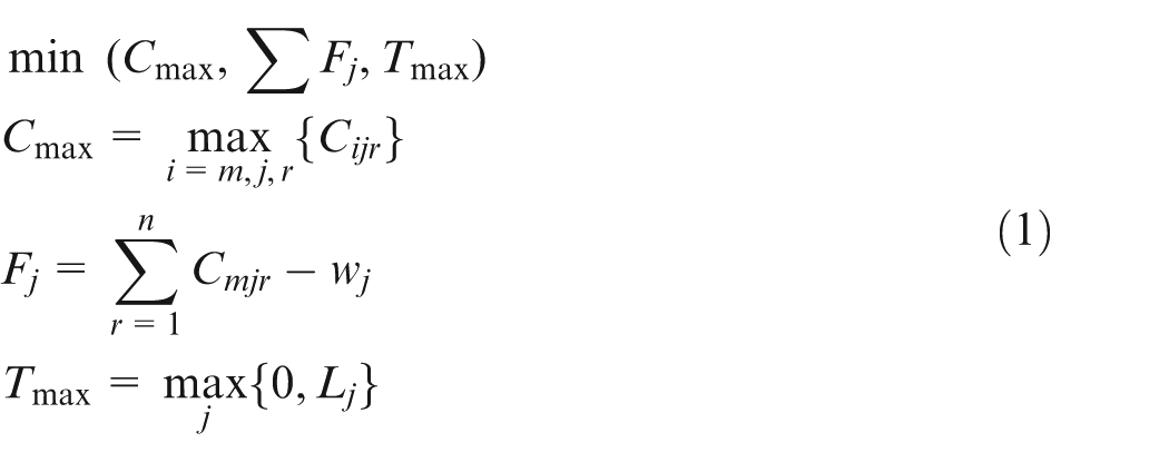
In equation (1), the objectives are defined as the makespan, sum of flow time and maximum tardiness, respectively

\begin{array}{l} \min (C_{\max}, \sum F_{j}, T_{\max}) \\ C_{\max} = \max_{i = m, j, r} {C_{i j r}} \\ F_{j} = \sum_{r = 1}^{n} C_{m j r} - w_{j} \\ T_{\max} = \max_{j} {0, L_{j}} \end{array}

(1)

\begin{array}{l} s . t . \\ \sum_{r = 1}^{n} x_{i j r} = 1 \forall i, \forall j \end{array}

(2)

\sum_{j = 1}^{n} x_{i j r} = 1 \forall i, \forall r

(3)

\begin{matrix} \sum_{j = 1}^{n} C_{ij (r + 1)} ⩾ \sum_{j = 1}^{n} C_{ijr} \\ + x_{ij (r + 1)} . (p_{ij (r + 1)} + S_{i (r + 1)}) \\ + \sum_{k = 1}^{K} y_{ikr} . t_{ik} \forall i, \forall r = 1, \dots, n - 1 \end{matrix}

(4)

\begin{matrix} \sum_{r = 1}^{n} C_{(i + 1) jr} ⩾ \sum_{r = 1}^{n} C_{ijr} \\ + x_{(i + 1) jr} . (p_{(i + 1) jr} + S_{(i + 1) r}) \\ \forall i = 1, \dots, m - 1, \forall j \end{matrix}

(5)

\sum_{r = 1}^{n} (C_{mjr} - d_{j} . x_{mjr}) = L_{j} \forall j

(6)

\begin{matrix} \sum_{r = 1}^{n} C_{[1] jr} ⩾ w_{j} \\ + \sum_{r = 1}^{n} x_{[1] jr} . (p_{[1] jr} + S_{[1] r}) \forall j \end{matrix}

(7)

C_{ijr} ⩽ H . x_{ijr} \forall i, \forall j, \forall r

(8)

\begin{matrix} x_{ijr} = {0, 1} \forall i, j, r \\ C_{ijr} ⩾ 0 \forall i, j, r \\ L_{j} ⩾ 0 \forall j \end{matrix}

(9)

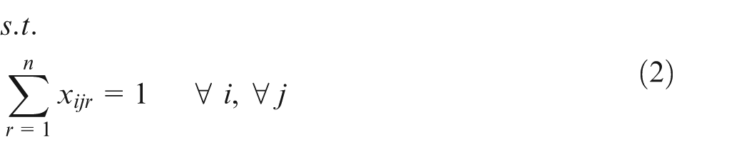
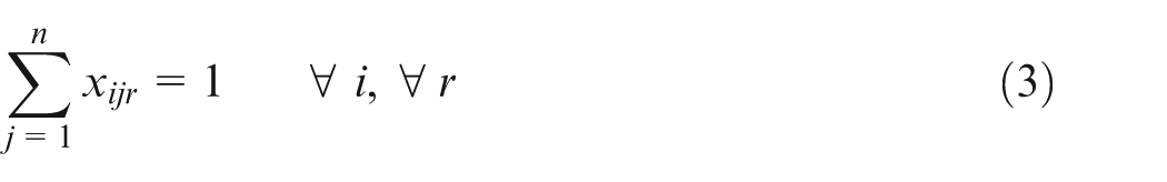
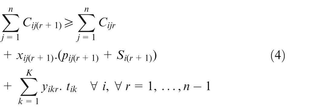
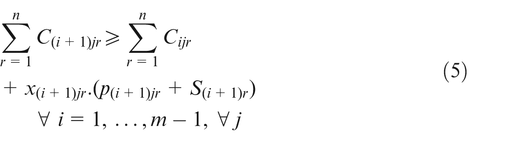
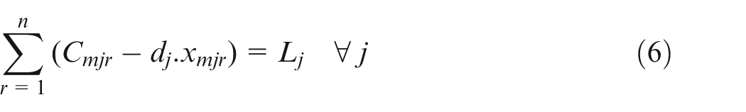
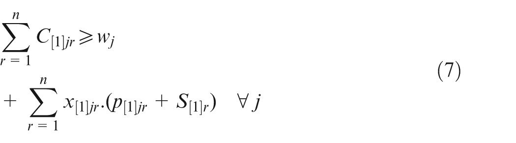
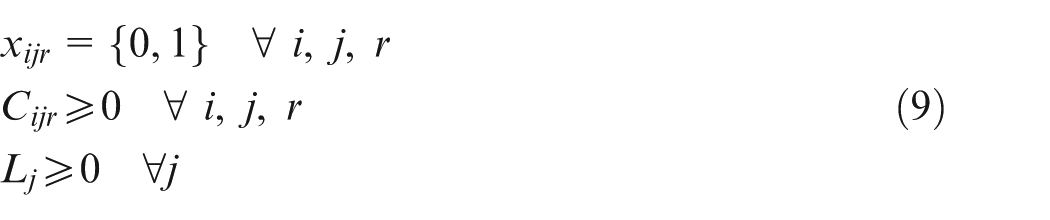
Equations (2) and (3) refer to the fact that on a particular machine, there is one job for each position and one position per job. Equation (4) states that the job in one position cannot finish before the completion of the job in the previous position. Additionally, if the maintenance activity k is scheduled on machine i for position r, then it should be done prior to the process of the job in the next position. Equation (5) is the concept of a flow shop problem, where a particular job should go through all machines one by one. Hence, the completion time of a job on the current machine is equal to or greater than its completion time on the previous machine plus its setup time and processing time on the current machine. Equation (6) defines the lateness of a job, that is, the difference between the completion time of a job on the last machine and its due date. Equation (7) defines the release date of each job. Note that this constraint is considered only on the first machine since when a job is about to start on the other machines, it has already surpassed its release date. Equation (8) ensures that the completion time of each job is either a logical positive number or it equals zero. That is, if a job is not processed in a certain position (i.e. if $x_{ijr}$ is zero), then its completion time on that particular position would be zero as well (i.e. its corresponding $C_{ijr}$ would be zero). On the other hand, if a job is processed in a specific position (i.e. if $x_{ijr}$ is one), then its completion time is a positive finite number smaller than the large number H. Finally, equation (9) states the decision variables.

Discussion on the model

In this section, the model presented above is examined in further details.

Learning effect

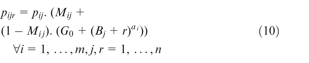
In the proposed model, the actual processing times of job j (i.e. $p_{ijr}$ ) is dependent on the machine i that it is processed on and its position r in the sequence of all jobs. This relation between the processing time and position of a job is due to the fact that positioning a (semi) manual job later in the sequence decreases the processing time of that job. This phenomenon is known as the learning effect. In other words, in a (semi) manual job, the operator gains experience with time and hence the time he or she needs to process a job gradually decreases up to a specific point. In this article, learning effect is formulated as follows

\begin{matrix} p_{ijr} = p_{ij} . (M_{ij} + \\ (1 - M_{i j}) . (G_{0} + (B_{j} + r)^{a_{i}})) \\ \forall i = 1, \dots, m, j, r = 1, \dots, n \end{matrix}

(10)

Here, $M (0 < M < 1)$ shows the portion of machine times of a job, that is, $M = 0$ refers to a completely manual job while $M = 1$ indicates a full automatic job.³ Parameter B, imported from Stanford-B learning curve,¹³ indicates the operator’s prior experience. Once the operator has mastered a job, the decrease in processing times comes to a halt. This stop is formulated using a truncation parameter, $G_{0} (0 < G_{0} < 1)$ , which controls the maximum reduction in processing times caused by learning effect. In equation (10), the values of $G_{0}$ , $B_{j}$ and $a_{i}$ should be given with care so that $G_{0} + (B_{j} + r)^{a_{i}} ⩽ 1$ .

Setup time

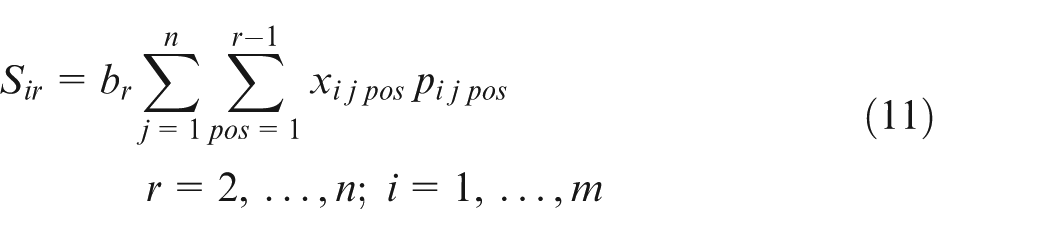
In this article, in addition to the position, psd setup time of a job is also dependent on the machine that the job is processed upon as follows⁵

\begin{matrix} S_{ir} = b_{r} \sum_{j = 1}^{n} \sum_{pos = 1}^{r - 1} x_{i j pos} p_{i j pos} \\ r = 2, \dots, n; i = 1, \dots, m \end{matrix}

(11)

In equation (11), $S_{ir}$ for a particular machine i and for a specific position r is a coefficient $(b_{r})$ of the total processing times of all the jobs in previous positions $(pos = 1, \dots, r - 1)$ on the same machine i. Hence, the later a job is processed, the longer its setup time. The example of such a case is in metallurgy industry where a certain high temperature is needed to operate a job. The temperature comes down with time so the longer a job is delayed, the longer it takes to increase the temperature back up again to the desired degree.

Discussion on the objectives

The key point in multi-objective problems is to choose the correct combination of objectives that can be considered together. The group of objectives selected cannot have direct relations with each other or else they are considered as one objective. In this article, the objectives are $C_{max}$ , $\sum F_{j}$ and $T_{max}$ . Simply put, $C_{max}$ is the bottleneck time, $\sum F_{j}$ is the total time of processing all jobs and $T_{max}$ is the maximum tardiness among the jobs. An increase (decrease) in $C_{max}$ leads to an increase (decrease) in $\sum F_{j}$ , but the reverse is not necessarily true. Thus, the relation between the two is not direct. Similarly, an increase in $C_{max}$ does not necessarily effect $T_{max}$ since the bottleneck job is not necessarily the job that resulted in the maximum tardiness. The relation between $\sum F_{j}$ and $T_{max}$ is not direct because $T_{max}$ might decrease, increase or stay indifferent to any changes in $\sum F_{j}$ . Hence, the three objectives can be considered together in a multi-objective problem.

The proposed algorithm

The proposed algorithm, namely, multi-objective simulated annealing differential evolution (MO-SADE), is a hybrid method which combines the multi-objective DE with the population-based SA. Similar to other evolutionary methods,¹⁴ the algorithm starts with a random population of real individuals from the continuous search region. Since the flow shop problem under study is discrete by nature, a technique is needed to convert the continuous solutions to job permutations and vice versa. After the initialization stage, the algorithm enters the main loop which includes an inner and outer loop. The inner loop uses $DE / best / 1 / bin$ strategy and two populations to find the non-dominated schedules. The outer loop utilizes the single-objective SA to find the extreme points in respect to each objective. Since SA is an additional search method, it is possible to run it conditionally for each generation, or for every 10 generation or just for the last generation. If this condition is met, the algorithm enters the SA loop; otherwise, it proceeds to the next DE generation. The framework of the algorithm can be outlined as follows. First, the problem and parameters should be defined: (a) set SA parameters: initial temperature $(T_{0})$ , maximum number of SA iterations $(Maxit_SA)$ , number of iterations for the inner loop of SA with a constant temperature $(Subit_SA)$ , the iterative reduction rate in temperature $(α)$ and the number of neighbors created for each individual $(Nsrch)$ . Here, $T_{G}$ is the temperature for each iteration G. (b) Set DE parameters: initial population size $(NP)$ , the upper bound on population individuals $(Va r_{\max})$ and lower bound $(Va r_{\min})$ , number of objectives $(Nobj)$ , maximum number of iterations $maxit (G = 1, \dots, maxit)$ scheduling model inputs for n jobs and m machines, crossover rate $(CR)$ , mutation control parameter $(F)$ . Additionally, set $bes t_{G}$ as the best individual in generation G and set $A d v a n c e d p o p u l a t i o n$ as an empty additional population.

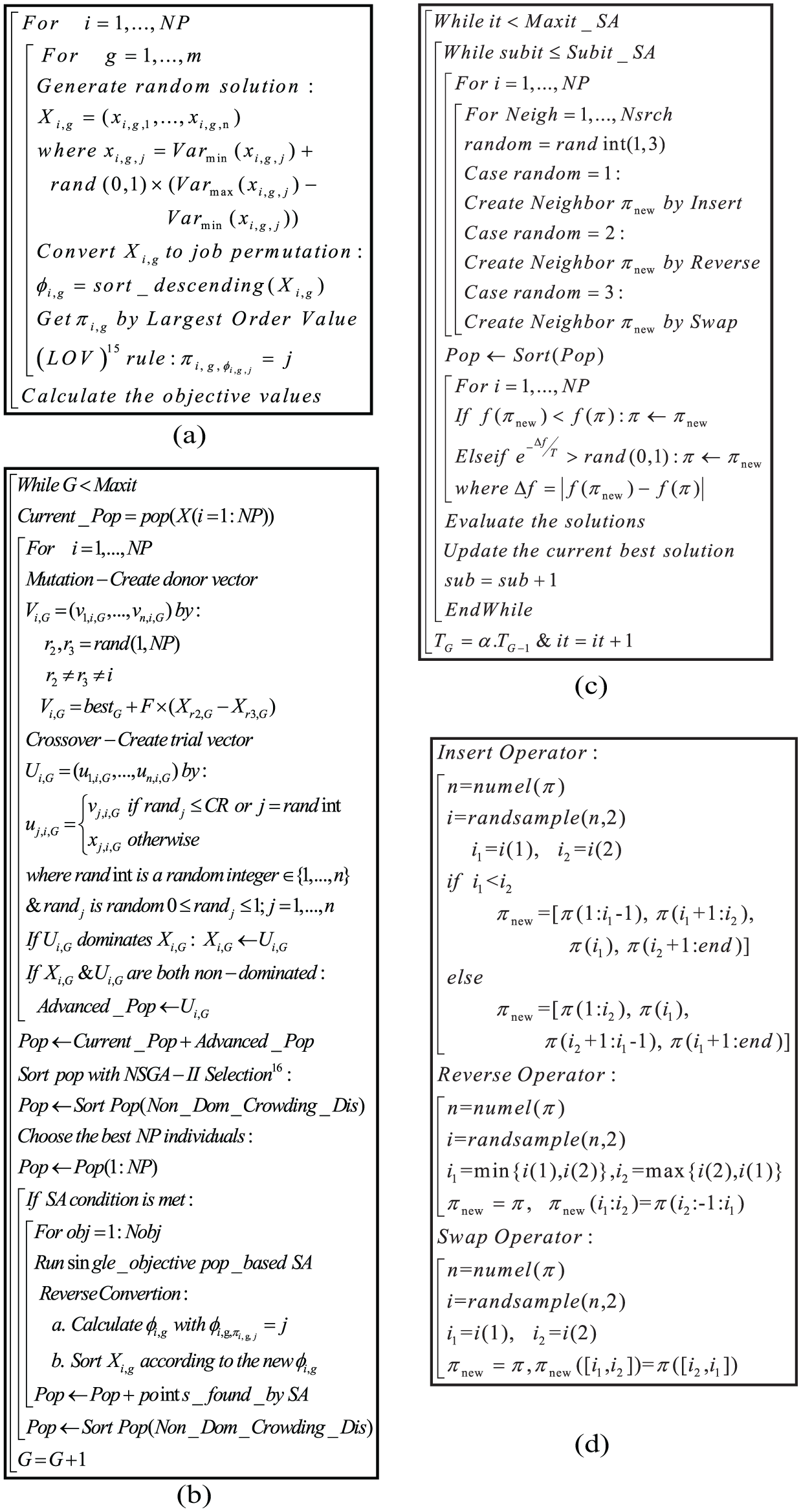
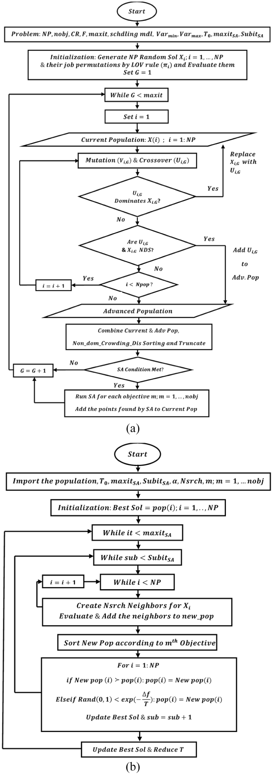
Next step is the initialization phase, followed by the main loop. The procedures for these steps are summarized in Figure 2(a) and (b), respectively. The flowchart of the algorithm is also illustrated in Figure 3(a). Similarly, SA starts by importing the population from DE. The main loop of SA is explained in Figure 2(c). The insert, reverse or swap operators for job permutation $π$ are defined in Figure 2(d) where $numel (π)$ is the number of elements in the permutation $π$ , $randsample (n, 2)$ chooses two integer values from n, called $i (1)$ and $i (2)$ , and $π_{new}$ is the neighbor created from the original permutation $π$ . In the population-based SA, instead of conducting the search on a single individual, SA is repeated for a population of individuals. The flowchart of the proposed SA is shown in Figure 3(b).

Figure 2.

(a) Initialization phase, (b) main loop of MO-SADE, (c) main loop of SA and (d) search operators of SA.

Figure 3.

(a) Framework of the proposed algorithm(MO-SADE) and (b) framework of population-based SA.

Constraint handling in MO-SADE

Consider the problem of three jobs on three machines with two maintenance activities. MO-SADE commences by generating a random sequence for each machine. The length of each sequence is the same as the number of jobs.

Hence, three random sequences are generated using uniform distribution for $Va r_{\max} = 10$ and $Va r_{\min} = 1$ as follows

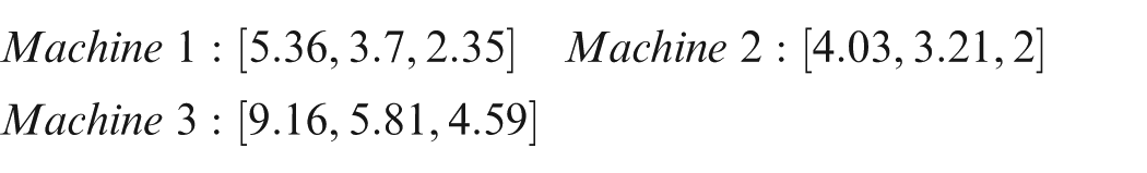
Machine 1 : [5.36, 3.7, 2.35] Machine 2 : [4.03, 3.21, 2] Machine 3 : [9.16, 5.81, 4.59]

According to the Largest Order Value (LOV) rule, the largest value in a sequence gets the first position. Since the random values are sorted decreasingly on all machines, the corresponding permutations are achieved as $[1, 2, 3]$ for all the machines. This solution is the equivalent of $x_{111} = x_{122} = x_{133} = 1$ for machine 1, $x_{211} = x_{222} = x_{233} = 1$ for machine 2 and $x_{311} = x_{322} = x_{333} = 1$ for the last machine.

Using the achieved values for $x_{ijr}$ , the processing times can be calculated using equation (10). For instance, $p_{122}$ can be achieved as follows

p_{122} = p_{12} (M + (1 - M) \times (G_{0} + (B + 2)^{- a}))

Similarly, setup times can also be calculated by equation (11). For instance, $S_{13}$ can be calculated as follows

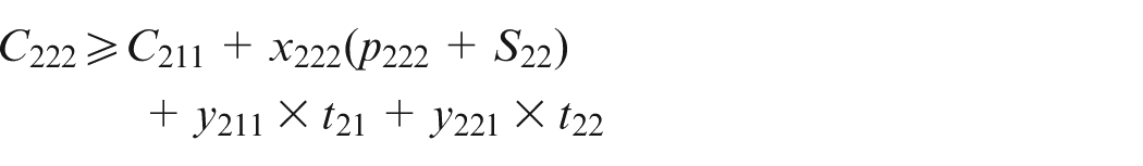
S_{13} = b_{3} \times (x_{111} p_{111} + x_{122} p_{122} + x_{133} p_{133})

Then, from constraints (4) and (5), $C_{ijr}$ would be achieved. For instance, according to equation (5), $C_{222}$ should satisfy the following equation

C_{222} ⩾ C_{122} + x_{222} (p_{222} + S_{22})

Simultaneously, $C_{222}$ should also consider the maintenance times mentioned in equation (4) as follows

\begin{matrix} C_{222} ⩾ C_{211} + x_{222} (p_{222} + S_{22}) \\ + y_{211} \times t_{21} + y_{221} \times t_{22} \end{matrix}

So basically, the maximum value between these two equations would be $C_{222}$ . Once the completion time of each job on the last machine is determined, the lateness of each job can be calculated by equation (6). For instance, $L_{1}$ is calculated as follows

L_{1} = C_{311} - d_{1} \times x_{311}

Since tardiness of a job is the maximum of zero and its lateness, then the tardiness of each job would be $T_{j} = max (0, L_{j})$ and from there the objective values can be calculated.

Computational experiments

In this section, first four performance metrics are suggested for evaluating the proposed algorithm. Then, MO-SADE parameters are calibrated with Taguchi method. Finally, MO-SADE is tested on random benchmark problems and the results are compared to those of other methods. The experiments are performed with CPU @ 1.70 GHz with 4 GB of RAM.

Performance metrics

Here, four performance metrics are suggested to evaluate the results.

Overall non-dominated vector generation

Overall non-dominated vector generation (ONVG) simply counts the number of solutions found in the true Pareto front.¹⁵ The idea behind this is that higher ONVG indicates better exploration.

Diversity metric (Δ)

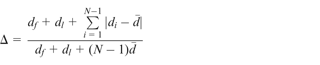
This metric gauges the distance between the solutions of a Pareto set to see how well spread the achieved points are. For N solutions of a set, it is defined as follows¹⁶

Δ = \frac{d_{f} + d_{l} + \sum_{i = 1}^{N - 1} | d_{i} - \bar{d} |}{d_{f} + d_{l} + (N - 1) \bar{d}}

where $d_{i} (i = 1, \dots, N - 1)$ is the Euclidean distance between consecutive solutions in the Pareto set and the average of these points is $\bar{d}$ . Here, $d_{f}$ and $d_{l}$ are the distances between the extreme solutions and the boundary solutions, respectively. The smaller Δ shows better performance.

Average quality metric

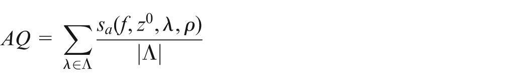
This performance metric measures the quality of the solutions achieved. It is formulated as follows¹⁵

AQ = \sum_{λ \in Λ} \frac{s_{a} (f, z^{0}, λ, ρ)}{| Λ |}

where

\begin{matrix} s_{a} (f, z^{0}, λ, ρ) = \min_{i} {\max_{j} {λ_{j} (f_{j} (x_{j}) - z_{j}^{0})} \\ + ρ \sum_{j = 1}^{ω} λ_{j} (f_{j} (x_{j}) - z_{j}^{0})} \end{matrix}

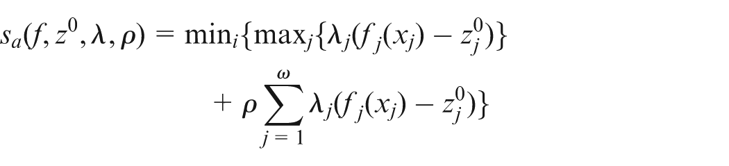
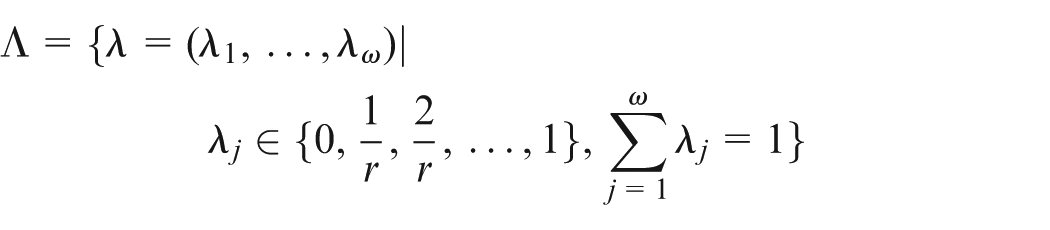
Here, $f_{j} (.)$ is the $j th$ objective in the ω-dimensional objective space where $i = 1, \dots, NP, j = 1, \dots, ω$ and $λ_{j}$ is defined by

\begin{matrix} Λ = {λ = (λ_{1}, \dots, λ_{ω}) | \\ λ_{j} \in {0, \frac{1}{r}, \frac{2}{r}, \dots, 1}, \sum_{j = 1}^{ω} λ_{j} = 1} \end{matrix}

where the reference point is set as $z^{0} = (0, 0)$ and $ρ = 0.01, r = 100$ . A smaller average quality (AQ) metric indicates better quality.

Convergence metric (γ)

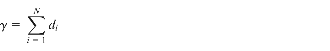
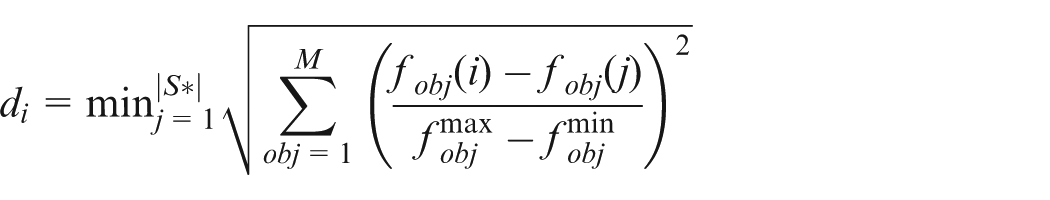
This metric measures the convergence of N individuals in the Pareto set toward a reference set $S^{*}$ . It is formulated as¹⁶

γ = \sum_{i = 1}^{N} d_{i}

where $d_{i}$ for the $i th$ solution is

d_{i} = \min_{j = 1}^{| S * |} \sqrt{\sum_{obj = 1}^{M} {(\frac{f_{obj} (i) - f_{obj} (j)}{f_{obj}^{max} - f_{obj}^{min}})}^{2}}

and M is the number of objectives. Here, $f_{obj}^{max}, f_{obj}^{min}$ are the maximum and minimum values of the $obj th$ objective, respectively. Smaller $γ$ indicates better performance.

Parameter calibration

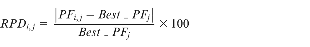
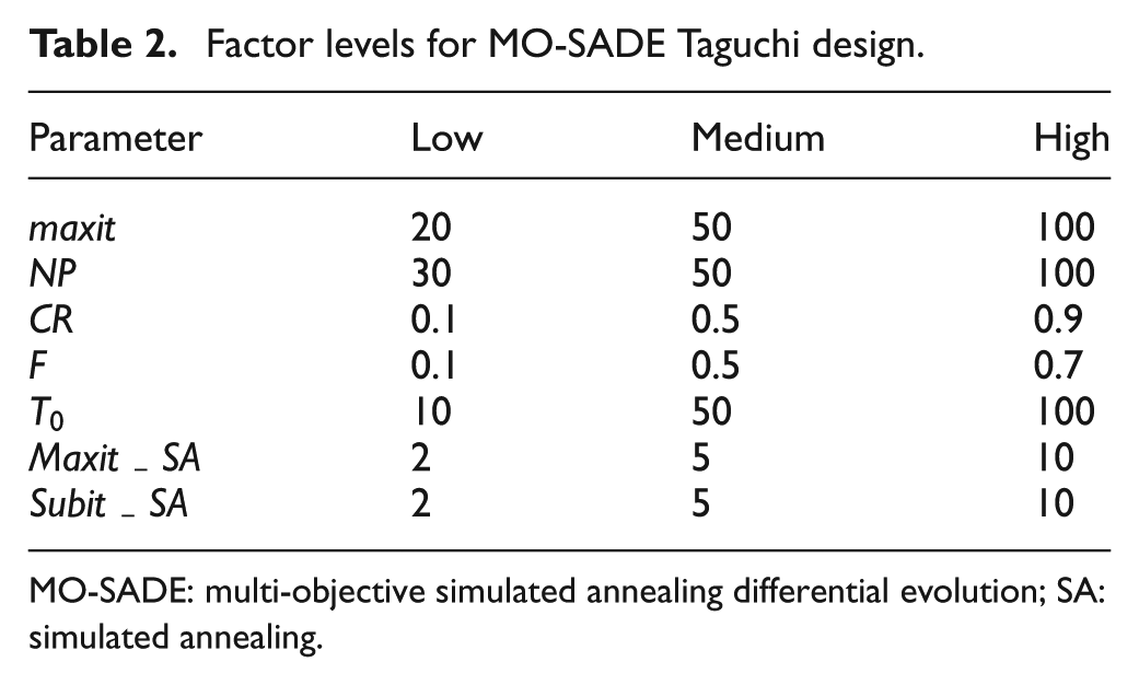
Similar to most meta-heuristics, MO-SADE is quite sensitive to its initial parameters. Here, the Taguchi method is used to determine the best combination of parameters in order to enhance the algorithm robustness. First seven factors are chosen and three levels are defined for each (Table 2). That returns $L_{27}$ orthogonal array for small and medium problems. Since the problem under study is multi-objective, first the experiments are carried out and then four performance metrics for each 27 experiments are calculated. Next, the values are scaled using the relative percentage deviation (RPD) concept as follows and the weighted average of them is used as a response

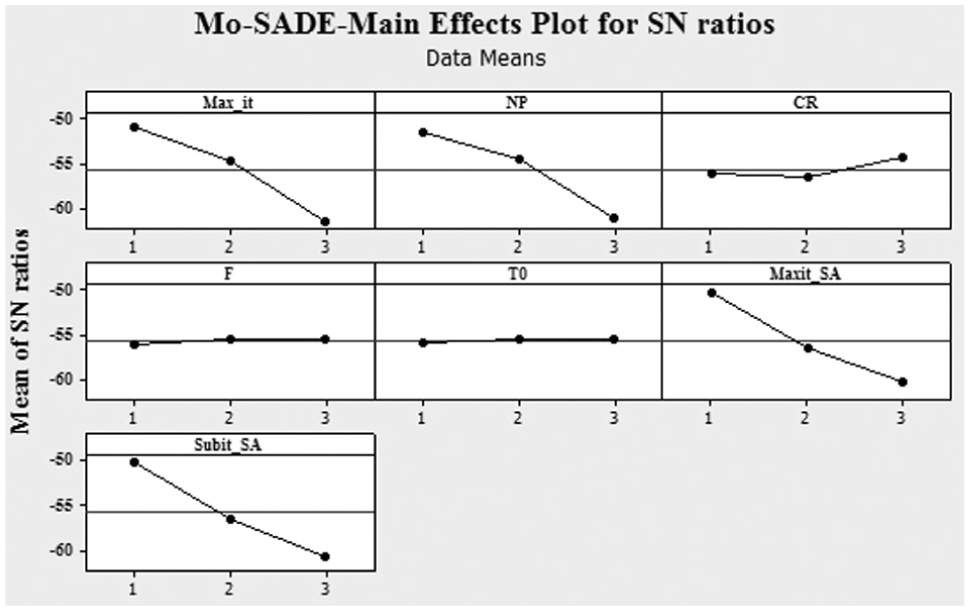
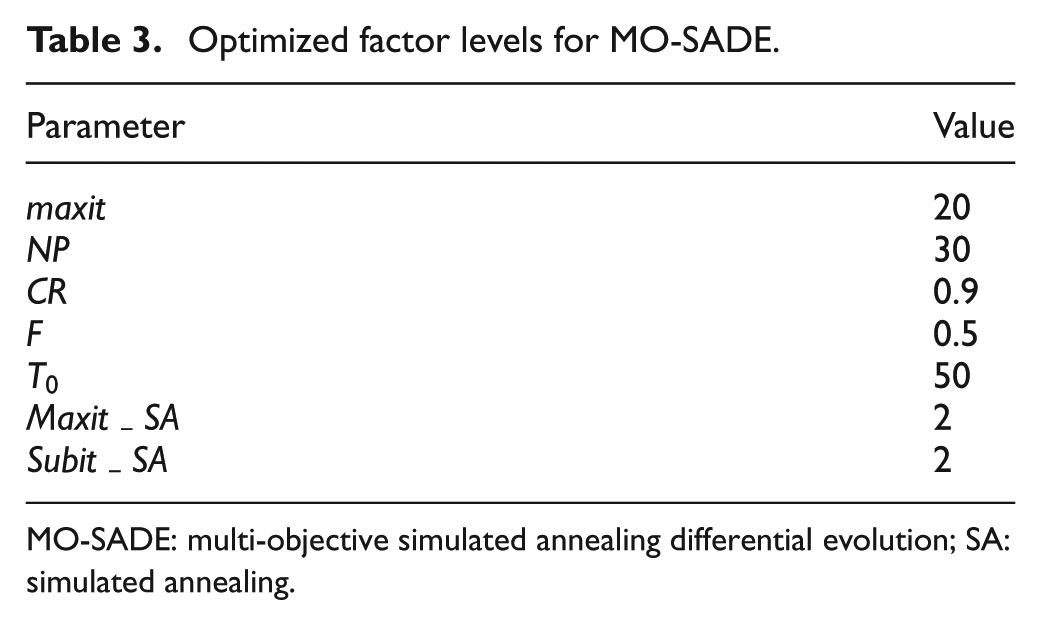
RP D_{i, j} = \frac{| P F_{i, j} - Best_P F_{j} |}{Best_P F_{j}} \times 100

where $RP D_{i, j}$ is the scaled value for experiment i of $j th$ performance metric $(P F_{j})$ . Similarly, $P F_{i, j}$ refers to the value of $j th$ performance metric of $i th$ run and $Best_P F_{j}$ is the best value among the values achieved for the $j th$ performance metric. Figure 4 shows the signal to noise (S/N) ratio achieved by the Taguchi analysis, respectively. The best level for each factor is the one with higher S/N ratio. Table 3 shows the optimized levels for each factor.

Table 2.

Factor levels for MO-SADE Taguchi design.

Parameter	Low	Medium	High
maxit	20	50	100
NP	30	50	100
CR	0.1	0.5	0.9
F	0.1	0.5	0.7
$T_{0}$	10	50	100
$Maxit_SA$	2	5	10
$Subit_SA$	2	5	10

MO-SADE: multi-objective simulated annealing differential evolution; SA: simulated annealing.

Figure 4.

S/N ratio plot.

Table 3.

Optimized factor levels for MO-SADE.

Parameter	Value
maxit	20
NP	30
CR	0.9
F	0.5
$T_{0}$	50
$Maxit_SA$	2
$Subit_SA$	2

MO-SADE: multi-objective simulated annealing differential evolution; SA: simulated annealing.

Discussion and results

In this section, for small and medium low problems, the proposed MO-SADE is compared with the exact values achieved by solving the mixed integer model using augmented ε-constraint method.^12,17 For medium high and large problems, MO-SADE is compared with two other meta-heuristics, that is, imperialist competitive algorithm (ICA) and multi-objective differential evolution scheduling (MDES).¹⁰ Problems are labeled as $Machine \times Job \times Maintenance$ , where the possible solutions for a problem equal to $(Job!)^{Machine} \times Maintenance$ . For example, the problem $3 \times 3 \times 2$ refers to a non-permutation flow shop problem with three machines, three jobs, two maintenance activities and $(3!)^{3} \times 2 = 432$ possible solutions. For simplicity, all the tests are carried out with 70% of learning $(a = - 0.152)$ .

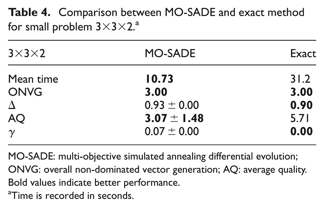
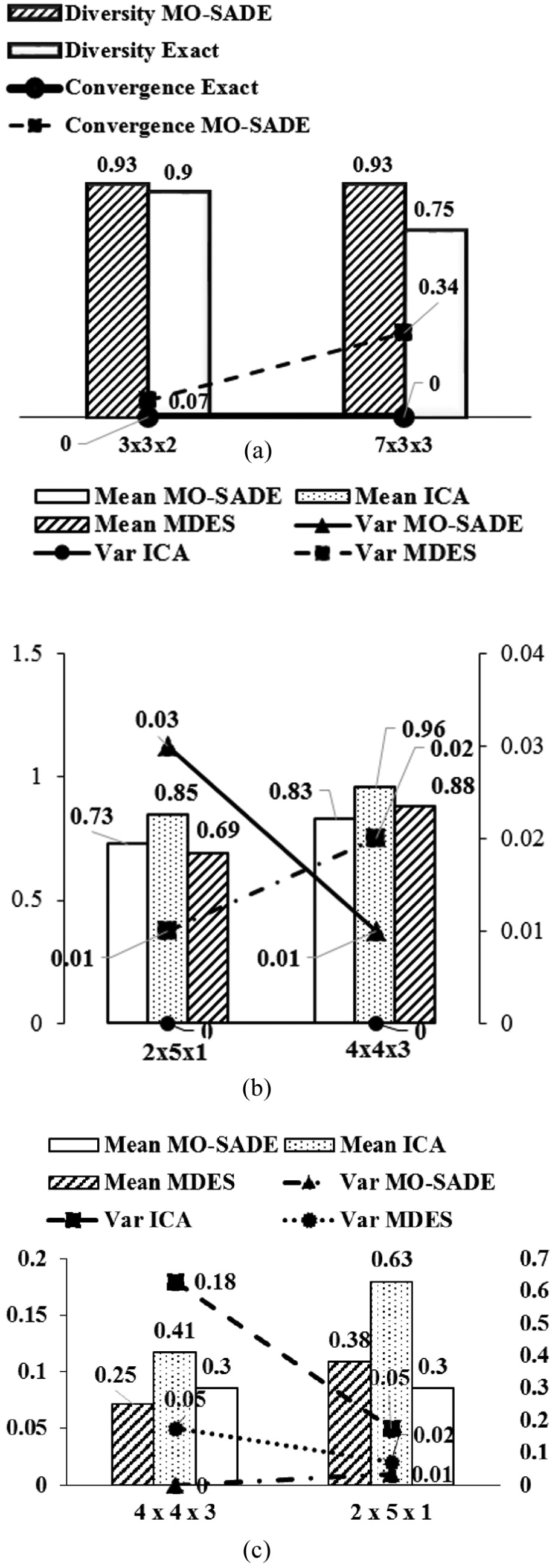
In this article, based on the time it takes to find a solution and the number of possible solutions, the problems are divided into four categories: (a) small: if the number of possible solutions does not have higher than three digits and a solution is found via the exact method under 1800 s; (b) medium low: if the number of possible solutions has between three and six digits and a solution is found via the exact method under 1800 s; (c) medium high: if the number of possible solutions has between three and six digits and a solution is not found by the exact method in 2400 s; (d) large: if the number of possible solutions has six digits or higher and a solution is not found by the exact method in 3000 s. One problem from each category is examined. Problem $3 \times 3 \times 2$ is a small problem which has 432 possible solutions and is solved in approximately 30 s by the exact method. Problem $7 \times 3 \times 3$ is medium low since it has 839,808 possible solutions but it is solved in 1120 s by the exact method. This is due to the fact that the run time is more sensitive to the number of jobs rather than the number of machines. Problem $2 \times 5 \times 1$ is an example of medium high problem with the possible solutions of 14,400 and it takes more than 2400 s to be solved by the exact method. Finally, problem $4 \times 4 \times 3$ is considered large with 995,328 possible solutions and run time of higher than 3000 s via the exact method (The specification of sample problems are available in the Appendix part at: http://le-scheduling.blogfa.com/page/JEM2016). The results are summarized in Tables 4 –7 and illustrated in Figure 5. As can be seen in Table 4, for problem $3 \times 3 \times 2$ , ONVG has the same value for MO-SADE and the exact method, which means similar exploration performance. The exact method performs marginally better than MO-SADE in diversity (3% difference in $Δ$ ) and also in convergence (7% difference in $γ$ ). On the other hand, MO-SADE performs faster than the exact method by approximately 20 s. Finally, MO-SADE has better balance between intensification and diversification than the exact method by 85% $(A Q_{MOSADE} = 3.07 < A Q_{Exact} = 5.71)$ .

Table 4.

Comparison between MO-SADE and exact method for small problem $3 \times 3 \times 2$ .^a

$3 \times 3 \times 2$	MO-SADE	Exact
Mean time	10.73	31.2
ONVG	3.00	3.00
$Δ$	0.93 ± 0.00	0.90
AQ	3.07 ± 1.48	5.71
$γ$	0.07 ± 0.00	0.00

MO-SADE: multi-objective simulated annealing differential evolution; ONVG: overall non-dominated vector generation; AQ: average quality.

Bold values indicate better performance.

Time is recorded in seconds.

Table 5.

Comparison between MO-SADE and exact method for medium problem $7 \times 3 \times 3$ .^a

$7 \times 3 \times 3$	MO-SADE	Exact
Mean time	44.75	1120.2
ONVG	3.20	4.00
$Δ$	0.93 ± 0.01	0.75
AQ	6.32 ± 2.54	6.25
$γ$	0.34 ± 0.10	0.00

MO-SADE: multi-objective simulated annealing differential evolution; ONVG: overall non-dominated vector generation; AQ: average quality.

Bold values indicate better performance.

Time is recorded in seconds.

Table 6.

Comparison between MO-SADE and other methods for medium high problem $2 \times 5 \times 1$ .^a

$2 \times 5 \times 1$	MO-SADE	ICA	MDES
Time	17.08	1.85	3.60
ONVG	7.70	2.20	7.20
$Δ$ ^b	0.73 ± 0.03	0.85 ± 0.00	0.69 ± 0.01
AQ	3.92 ± 1.40	5.65 ± 11.9	4.21 ± 0.59
$γ$	0.30 ± 0.00	0.63 ± 0.18	0.38 ± 0.05

MO-SADE: multi-objective simulated annealing differential evolution; ICA: imperialist competitive algorithm; MDES: multi-objective differential evolution scheduling; ONVG: overall non-dominated vector generation; AQ: average quality.

Bold values indicate better performance.

Time is recorded in seconds.

The results are average of 10 runs.

Table 7.

Comparison between MO-SADE and other methods for large problem $4 \times 4 \times 3$ .^a

$4 \times 4 \times 3$	MO-SADE	ICA	MDES
Time	34.70	2.76	4.99
ONVG	4.30	1.90	3.90
$Δ$ ^b	0.82 ± 0.01	0.96 ± 0.00	0.88 ± 0.02
AQ	4.31 ± 2.37	5.90 ± 3.58	4.33 ± 1.380
$γ$	0.30 ± 0.01	0.41 ± 0.05	0.25 ± 0.02

Bold values indicate better performance.

Time is recorded in seconds.

The results are average of 10 runs.

Figure 5.

(a) Comparison between the exact method and MO-SADE for a small $(3 \times 3 \times 2)$ problem and a medium low problem $(7 \times 3 \times 3)$ , (b) mean and variance diversity metric comparison of medium high $(2 \times 5 \times 1)$ and large problem $(4 \times 4 \times 3)$ and (c) mean and variance convergence metric comparison of medium high $(2 \times 5 \times 1)$ and large problem $(4 \times 4 \times 3)$ .

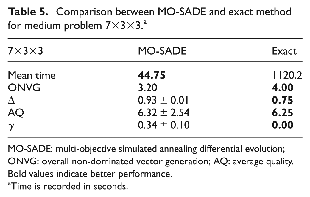
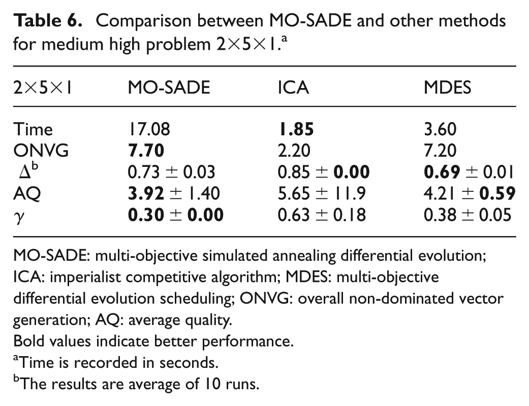
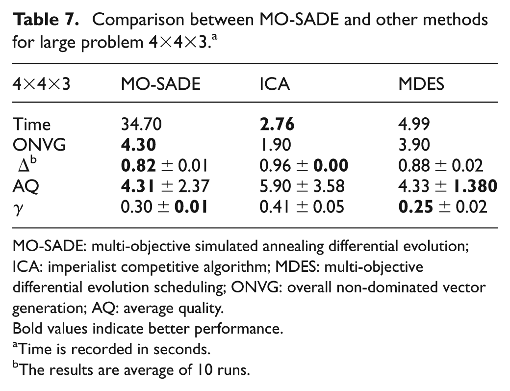
The test results on medium low problem $7 \times 3 \times 3$ are shown in Table 5. For this problem, the exact method performs better but it takes 25 times more seconds to solve the problem since MO-SADE takes 44.75 s to solve the problem while the exact method needs 1120.2 s to find similar results. The differences between the exact method and MO-SADE in regard to the exploration $(ONVG)$ , diversity $(Δ)$ , convergence $(γ)$ and quality of solutions $(AQ)$ are 8%, 18%, 34% and 7%, respectively, with the exact method being in the lead. These differences are relatively small in regard to approximately 1075 more seconds needed to achieve better results. In Figure 5(a), the differences in convergence and diversity of exact method and MO-SADE are illustrated for small and medium low problems, where the lower values are preferred. As can be seen, the exact method is slightly better than the proposed meta-heuristic both in convergence and diversity. However, exact method has high computational time, hence the use of MO-SADE in larger problems. For consistency, in medium high and large problems, the stopping criteria and population size for all algorithms are set to 20 iterations and 30 individuals, respectively. In Table 6, for the medium high problem $2 \times 5 \times 1$ , MO-SADE is compared with ICA and MDES. For this problem, from Table 6, it can be seen that ICA is the fastest method with run time of 1.85 s. However, the quality of solutions found by ICA is quite low. The ONVG achieved by ICA is 2.20 which is approximately 5 units less than the ONVG of MO-SADE (i.e. 7.70) and MDES (i.e. 7.20). Since higher ONVG is an indicator of better exploration, it can be concluded that MO-SADE has the best exploration among the methods, followed closely by MDES and with a wide gap by ICA. As for diversity metric $(Δ)$ , lower values are more desirable. As can be seen in the third row of Table 6, MO-SADE and MDES have nearly identical values in diversity metric (approximately 0.7) whereas diversity metric for ICA is quite high (i.e. 0.85) which shows the worst diversity. The quality metric AQ indicates overall quality of the solutions and lower values of this metric are desirable. As can be seen in Table 6, MO-SADE has the best quality (lowest AQ = 3.92), followed by MDES (AQ = 4.21) and finally ICA (AQ = 5.65). In other words, in regard to the quality of solutions, MO-SADE is superior to MDES and ICA by 7% and 44%, respectively. In regard to convergence $(γ)$ , MO-SADE finds the lowest value $(γ = 0.3)$ which indicates the best precision among the algorithms. This means MO-SADE is superior to MDES and ICA with the differences of 10% $(γ = 0.4)$ and 50% $(γ = 0.8)$ , respectively. In Table 7, for the problem $4 \times 4 \times 3$ , ICA is once again the fastest algorithm with the run time of about 3 s, closely followed by MDES with run time of approximately 5 s. However, MO-SADE takes about 11 times longer than ICA and 7 times longer than MDES to find the solutions. This rise in computational time is justified by a rise in quality of achieved solutions.

On the account of exploration, MO-SADE has the highest ONVG $(ONVG = 4.3)$ , which shows better exploration of the search than MDES $(ONVG = 3.9)$ and ICA $(ONVG = 1.9)$ by 9% and 55%, respectively. As can be seen in the third row of Table 7, MO-SADE has the lowest $Δ$ which means the best diversity among the algorithms $(Δ = 0.83)$ . This means MO-SADE is superior to MDES and ICA with the differences of 5% $(Δ = 0.88)$ and 8% $(Δ = 0.96)$ , respectively. The fourth row of Table 7 gauges the quality of solutions. MO-SADE and MDES have almost the same quality (4.31 and 4.33, respectively) which is much better than that of ICA with quality metric of 5.90 by 37%. However, MDES achieves a better convergence metric $(γ)$ than MO-SADE and ICA with the difference of 5% and 16%, respectively. Figure 5(b) and (c) shows the comparison between the diversity and convergence of MO-SADE, MDES and ICA for medium high and large problems, respectively, where lower values are desired. As can be seen in Figure 5(b), MO-SADE and MDES have similar performance and ICA has the worst mean diversity among the methods. The difference in variances is at most 3% which is an inconsequential gap so it can be concluded that all the algorithms are relatively similar in robustness of diversity metric.

Similarly, in Figure 5(c), MO-SADE has the lowest variances, which means it is the most robust algorithm, followed by MDES and ICA, respectively. On mean convergence, MO-SADE and MDES have similar performance and ICA has the worst performance.

An example on effect of SA in MO-SADE

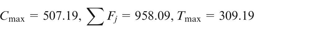
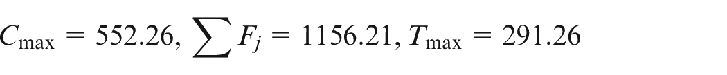
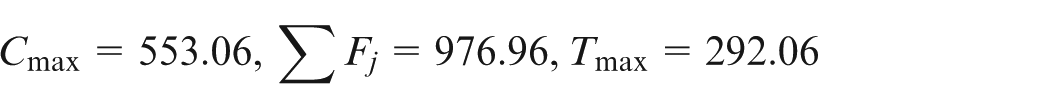
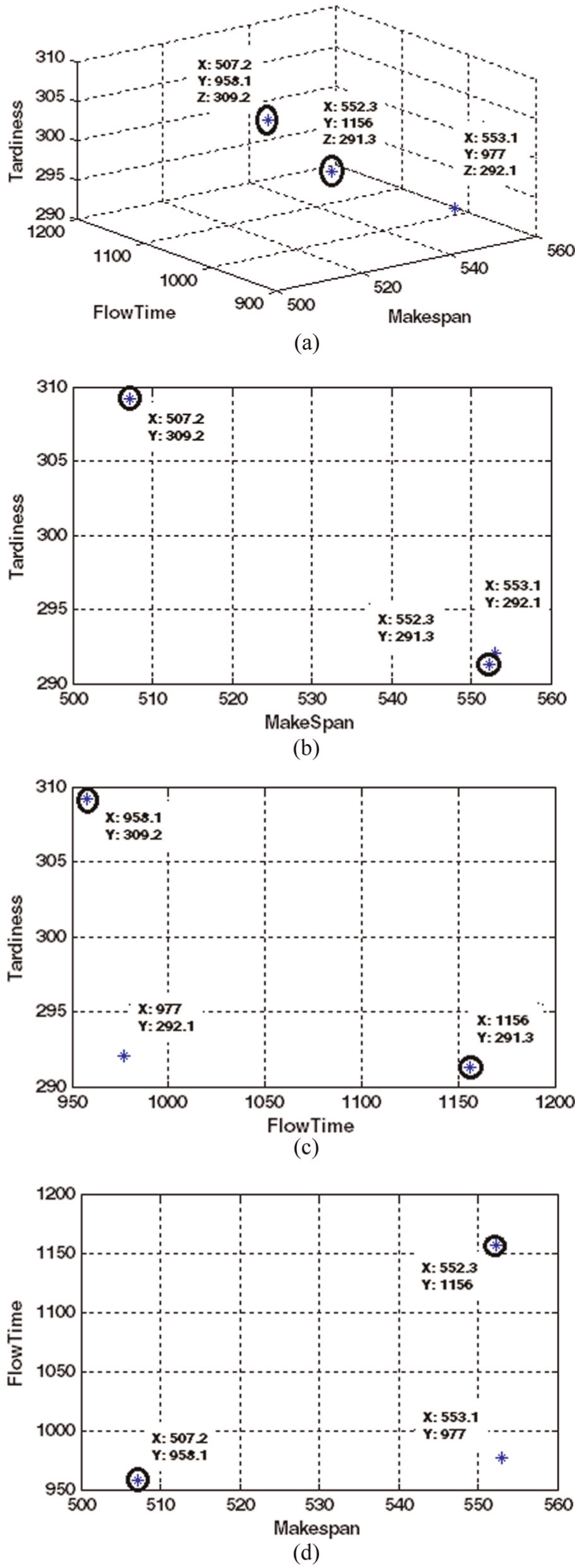
In this section, the behavior of the algorithm is examined for the small problem $3 \times 3 \times 2$ . This problem has three non-dominated solutions as follows:

Solution 1

C_{max} = 507.19, \sum F_{j} = 958.09, T_{max} = 309.19

Solution 2

C_{max} = 552.26, \sum F_{j} = 1156.21, T_{max} = 291.26

Solution 3

C_{max} = 553.06, \sum F_{j} = 976.96, T_{max} = 292.06

According to our computations, SA finds the extreme values of makespan, sum of flow time and maximum tardiness as 507.19, 958.09 and 291.26, respectively. These values are shown in solutions 1 and 2. Solution 3 is found by DE, which is quite similar to Solution 2. In other words, DE finds a non-dominated neighbor for the extreme points found by SA. This can also be seen in Figure 6, where the extreme points found by SA are circled and the rest are found by DE. The three side views help to see the location of each point in respect to different objectives. In the first side view (makespan vs tardiness), the circled point of $C_{max} = 552.26$ and $T_{max} = 291.26$ , found by SA, is quite near to the point above it, $C_{max} = 553.06$ and $T_{max} = 292.06$ , which is found by DE. In other words, DE has balanced the exploration between objectives by worsening $C_{max}$ and $T_{max}$ a little, while finding a better value for the third objective as follows and thus creating a third non-dominated point: $(\sum F_{j})_{DE} = 976 < (\sum F_{j})_{SA} = 1156$ . In summary, the idea behind inserting SA to DE is the fact that DE progresses with a balanced exploration. In other words, it finds a solution which minimizes all the objectives best. Consequently, it takes a long time to find the extreme points for each objective. On the other hand, since SA is run for a single objective, it can find the extreme values with ease. Note that extreme values of each objective are always included in the true Pareto front. Hence, by imbedding SA in DE, the extreme points are added to the population in each generation. Then, DE takes over and finds the neighbors of the extreme values, thus creating a converged and diverse Pareto front.

Figure 6.

Points found by SA and DE for problem $3 \times 3 \times 2$ .

Conclusion

In this article, a general flow shop problem is addressed where the jobs’ processing times and psd setup times are affected by a modified learning effect. Since the problem is strongly NP-hard, it was tackled by a multi-objective DE algorithm based on simulated annealing (named MO-SADE). The population-based SA imbedded in the algorithm is run once for each objective with the solo minimization of that particular objective in mind. Adding SA to DE improved the exploration and resulted in a well-converged and diverse Pareto solution. When compared with other methods, MO-SADE showed better balance between convergence and diversity. An extension of the current problem in job shop or flexible flow shop scheduling might be an interesting topic for future research.

Footnotes

Declaration of conflicting interests

The author(s) declared no potential conflicts of interest with respect to the research, authorship and/or publication of this article.

Funding

The author(s) received no financial support for the research, authorship and/or publication of this article.

References

Seidgar

Zandieh

Fazlollahtabar

. Simulated imperialist competitive algorithm in two-stage assembly flow shop with machine breakdowns and preventive maintenance. Proc IMechE, Part B: J Engineering Manufacture. Epub ahead of print 18 February 2015. DOI: 10.1177/0954405414563554.

Bahalke

Dolatkhahi

Dehghani

. Formulation and heuristic algorithm for flow time minimization in a simple assembly line. Proc IMechE, Part B: J Engineering Manufacture 2012; 226(3): 512–526.

Okolowski

Gawiejnowicz

Exact and heuristic algorithms for parallel-machine scheduling with DeJong’s learning effect. Comput Ind Eng 2010; 59(2): 272–279.

Zandieh

Fatemi Ghomi

SMT

Moattar Husseini

SM.

An immune algorithm approach to hybrid flow shops scheduling with sequence-dependent setup times. Appl Math Comput 2006; 180(1): 111–127.

Amirian

Sahraeian

Augmented ε-constraint method in multi-objective flowshop problem with past sequence set-up times and a modified learning effect. Int J Prod Res 2015; 53(19): 5962–5976.

Sun

Zhang

Gao

. Multi-objective optimization algorithms for flow shop scheduling problem: a review and prospects. Int J Adv Manuf Tech 2011; 55(5–8): 723–739.

Yenisey

Yagmahan

Multi-objective permutation flow shop scheduling problem: literature review, classification and current trends. Omega 2013; 45: 119–135.

Dai

Tang

. Energy-aware integrated process planning and scheduling for job shops. Proc IMechE, Part B: J Engineering Manufacture 2014; 229(1): 13–26.

Rui

Shilong

Zheqi

. An ant colony algorithm for job shop scheduling problem with tool flow. Proc IMechE, Part B: J Engineering Manufacture 2014; 228(8): 959–968.

10.

Amirian

Sahraeian

Multi-objective differential evolution for the flow shop scheduling problem with a modified learning effect. Int J Eng Trans C 2014; 27(9): 1395–1404.

11.

Kirkpatrick

Gelatt

Vecchi

MP.

Optimization by simulated annealing. Science 1983; 220: 671–680.

12.

Mavrotas

Effective implementation of the ε-constraint method in multi-objective mathematical programming problems. Appl Math Comput 2009; 213(2): 455–465.

13.

Fogliatto

Anzanello

MJ.

Learning curves: the state of the art and research directions. In: Jaber

(ed.) Learning curves: theory, models, and applications, Boca Raton, FL, 2011, pp.3–15. Canada: CRC Press and Taylor & Francis Group.

14.

Zhou

Jiang

Yang

. A hybrid approach for multi-weapon production planning with large-dimensional multi-objective in defense manufacturing. Proc IMechE, Part B: J Engineering Manufacture 2014; 228(2): 302–316.

15.

Qian

Wang

Huang

. An effective hybrid DE-based algorithm for multi-objective flow shop scheduling with limited buffers. Comput Oper Res 2009; 36(1): 209–233.

16.

Deb

Pratap

Agarwal

. A fast and elitist multi-objective genetic algorithm: NSGA-II. IEEE T Evolut Comput 2002; 6(2): 182–197.

17.

Zhang

Reimann

A simple augmented ∈-constraint method for multi-objective mathematical integer programming problems. Eur J Oper Res 2014; 234(1): 15–24.

A hybrid differential evolution for general multi-objective flow shop problem with a modified learning effect

Abstract

Keywords

Introduction

Brief introduction on multi-objective problems

Mathematical formulation

Discussion on the model

Learning effect

Setup time

Discussion on the objectives

The proposed algorithm

Constraint handling in MO-SADE

Computational experiments

Performance metrics

Overall non-dominated vector generation

Diversity metric (Δ)

Average quality metric

Convergence metric (γ)

Parameter calibration

Discussion and results

An example on effect of SA in MO-SADE

Conclusion

Footnotes

Declaration of conflicting interests

Funding

References