Sage Journals: Discover world-class research

Abstract

Radio frequency identification is a developing technology that has recently been adopted in industrial applications for identification and tracking operations. The radio frequency identification network planning problem deals with many criteria like number and positions of the deployed antennas in the networks, transmitted power of antennas, and coverage of network. All these criteria must satisfy a set of objectives, such as load balance, economic efficiency, and interference, in order to obtain accurate and reliable network planning. Achieving the best solution for radio frequency identification network planning has been an area of great interest for many scientists. This article introduces the Ring Probabilistic Logic Neuron as a time-efficient and accurate algorithm to deal with the radio frequency identification network planning problem. To achieve the best results, redundant antenna elimination algorithm is used in addition to the proposed optimization techniques. The aim of proposed algorithm is to solve the radio frequency identification network planning problem and to design a cost-effective radio frequency identification network by minimizing the number of embedded radio frequency identification antennas in the network, minimizing collision of antennas, and maximizing coverage area of the objects. The proposed solution is compared with the evolutionary algorithms, namely genetic algorithm and particle swarm optimization. The simulation results show that the Ring Probabilistic Logic Neuron algorithm obtains a far more superior solution for radio frequency identification network planning problem when compared to genetic algorithm and particle swarm optimization.

Keywords

Radio frequency identification radio frequency identification network planning redundant antenna elimination Ring Probabilistic Logic Neuron genetic algorithm particle swarm optimization

Introduction

In recent decades, the advancement in technology and the use of modern engineering systems in industries from the production to transportation sector have inspired the need to track and identify materials, products, and even live subjects.¹ Radio frequency identification (RFID) technology can be addressed as one of the most reliable and efficient solutions for tackling this problem. RFID technology is known as an automatic identification technology because it uses wireless radio frequency waves that are produced by an electromagnetic field to transfer data for tracking and identifying objects. This technology can be implemented in different fields such as tracking and identifying patients in hospitals,² warehouse items tracking,³ tracking pallets and cases in shipment,⁴ monitoring production line,⁵ and manufacturing control system.⁶

In many applications, the deployment of RFID systems has generated a radio frequency identification network planning (RNP) problem⁷ which needs to be resolved, in order to efficiently operate a large-scale network. However, RNP is one of the most challenging problems that has to meet many requirements of the RFID system.^8,9 In general, the RNP aims to optimize a set of objectives (coverage, load balance, economic efficiency and interference between antennas, etc.) simultaneously; this is achieved by adjusting the control variables (the coordinates of the readers, the number of antenna, etc.) of the system. As a result, in a large-scale deployment environment, the RNP problem is a high-dimensional nonlinear optimization problem that has a vast number of variables and uncertain parameters.

Tracking and identifying objects in these applications require the deployment of several RFID antennas in the RNP, and the numbers of these antennas are calculated through the use of a mathematical model.^10–12 In the past, one of the typical ways to address the RNP problem was using a trial-and-error approach, which was an inaccurate and inefficient solution for such an important issue.^7,13,14 In addition, this approach could only be used on small-scale RNP problems.¹⁰ Nowadays, with the developments in computer technology, and software engineering, the conventional trial-and-error approach has been replaced with modern computational techniques that provide such important criteria like coverage of objects, collision of antennas, and number of antenna.¹⁵ Computational evolutionary techniques, such as artificial neural networks,¹⁶ fuzzy logic,¹⁷ genetic algorithm (GA),^10,11,18 particle swarm optimization (PSO),^13,19,20 differential evolution (DE),⁹ and hierarchical artificial bee colony algorithm,⁸ are points of interest for many scientists working with the RNP problem. In this respect, H Feng et al.²¹ proposed a novel optimization algorithm, namely, the multi-community GA-PSO for solving the complicated RNP problem. H Chen et al.⁷ developed an optimization model for planning the positions of the readers in the RNP based on PSO. Nawawi et al.²² proposed solution based on the PSO correlation between RNP parameters. S Lu and S Yu²³ proposed an approach based on k-coverage for RFID network planning, a k-coverage model is formulated from a multi-dimensional optimization problem and plant growth simulation algorithm, this is used to optimize the RFID networks by determining the optimal adjustable parameters. Y-J Gong et al.¹³ used the PSO algorithm with redundant reader elimination for optimizing the RNP.

The literature review by the authors indicates that the majority of the studies that have been conducted take into consideration the number of antennas as predefined by experts; however, this cannot be changed during the optimization process. Therefore, the ultimate goal of RNP is to calculate the number of antennas in a cost-efficient manner. In order to plan a cost-efficient RFID network, it is necessary to minimize the number of antennas, minimize the interference of antennas, and maximize the coverage area of objects.^11,16 Therefore, in this article, the Ring Probabilistic Logic Neuron (RPLN) is introduced as an efficient optimization technique to deal with the complex RNP problems; also, the RPLN has an inherent capability to adjust number of embedded RFID antennas in the network. In addition, to enable the RFID network model to be flexible with the number of antennas as well as reduce the optimizing process, redundant antenna elimination (RAE) is used before starting the optimization process. In each step of the optimization, all redundant antennas will be eliminated, and the optimization of the network will be applied to only non-redundant antennas.

The rest of this article is organized as follows: first, the RFID network model is introduced; next, the GA optimization technique is utilized to solve and optimize the RNP; third, the PSO approach is used to deal with RNP; following this is optimization of the proposed RNP by RPLN optimization technique; and finally, the results are compounded and compared.

RNP

An RFID system is made of four major elements, which are tags, readers, antennas, and computer unit. RFID configuration system is shown in Figure 1. It should be noted that the antenna could be a part of the reader; in that case, more than one antenna could be connected to one reader. Readers through antennas collect the data sent by tags and relay this to a host computer to process for further implementations. In essence, the RFID is the technology of processing data, which are radio frequency signals omitted from mounted tags on subjects and sent by readers to a host computer unit.²⁴ There are three types of tags: passive, semi-passive, and active. Differences between these three types of tags are based on their power source; in the sense that active and semi-passive tags are battery-powered, while passive tags do not have internal power.²⁵

Figure 1.

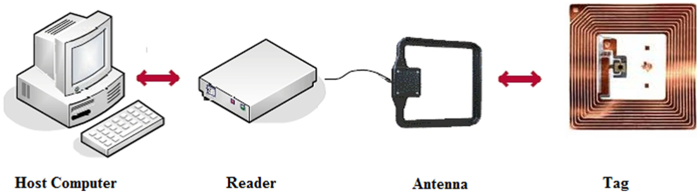
Components of RFID network.

It should be noted that passive tags have several advantages over semi-passive and active tags. First, passive tags are highly cost-effective and, second, they have a very long life cycle;²⁶ therefore, in this research, passive tags are used.

The distance between tag and antenna plays a major role in establishing communication between them. This problem exists because of the limit placed on the interrogation ranges of the antennas.²⁷ A reader can receive the information of a tag through antenna only in a limited range; because of this limitation, more than one antenna is used in many RFID systems to establish communication between tag and antenna. In such systems, many important objects like the number of antennas and their positions need to be thoroughly calculated. Answering such questions leads to an important concept named RNP.^13,23

Mathematical modeling of RFID network planning

A reliable RFID network model must be able to calculate coverage percentage of the tags, total transmitted power by antennas, and total interference of the network. The Friis transmission equation²⁸ is a well-known equation to formulate RFID network and has been used by many researchers to solve the RNP problem.^13,29,30 In this article, a developed model of this equation, which was proposed by Gong et al.,¹³ is utilized to calculate the main parameters of an RFID network such as the number of antennas, coverage area, and collision of antennas.

In order to define an RFID network model, the following steps should be taken:

Defining a working area;

Illustrating the number of distributed tags in this working area;

Defining the number of utilized antennas in this area.

In this article, the working area is defined as a square, that is, 100 × 100-m² rooms, where 20 passive tags are distributed in the room. It should be noted that the number of antennas here is arbitrary and can be chosen as any numbers. Predefined number of antennas, which are randomly distributed in the room, is assumed to be 20 at least, which is equal to the number of tags. Figure 2 shows the working area.

Figure 2.

Working area and distributed 20 tags.

After defining the parameters of the RFID network, the next step is calculating the properties of the network, which is the percentage of the covered tags by the antennas, number of redundant antennas, interference amount of antennas, and the total transmitted power by antennas.

Coverage

Coverage of a network is defined as the percentage of the tags, which are covered by deployed antennas, and so the ultimate goal of RNP is to achieve a 100% coverage of tags. As stated earlier, the tags considered in this article are passive tags, so they lack a power supply to produce radio frequency (RF) waves to communicate with antennas. Passive tags have internal circuits, which are activated when they receive electromagnetic waves that are greater than their power threshold, and so the activated tags start sending a backscatter signal and commence communication with the antennas.³¹

It can be said that a passive tag is covered by an antenna in the following manner:

A tag receives a signal from an antenna with the power of PT_a,t which is greater than the threshold value of the power of the tag (T_t).

This signal activates the tag, and then, the tag starts sending a backscatter signal to antennas with power of PA_t,a.

If the power of the backscatter signal is greater than the threshold value of the antenna power (T_a), then it can be said that the tag is covered by the antenna (Figure 3).

Figure 3.

Example of tag coverage.

The mathematical representation of the coverage of a tag is defined by following formula

C_{v} (t) = {\begin{matrix} 1, if \exists a_{1}, a_{2} \in AS, P T_{a_{1}, t} \geq T_{t} \land P A_{t, a_{2}} \geq T_{a} \\ 0, otherwise \end{matrix}

(1)

If there are N tags in a network, then the total percentage of coverage of the RFID network is defined as follows

C O V = \sum_{t \in T S} \frac{C_{v} (t)}{N_{t}} \times 100 %

(2)

where N_t = 20 and $1 \leq t \leq 20$ .

Figure 3 shows an example of tag coverage if $P T_{a_{1}, t_{n}} \geq T_{t_{n}} \land P A_{t_{n}, a_{3}} \geq T_{a_{3}}$ , then C_v(1) = 1. The received power by tags PT_a,t and transmitted power by tags PA_t,a are calculated through Friis transmission equation as shown below

P T_{a, t} [dBm] = P_{1} [dBm] + G_{a} [dBi] + G_{t} [dBi] - L [dB]

(3)

L [dB] = 10 \log [{(\frac{4 π}{λ})}^{2} d^{n}] + δ [dB]

(4)

\begin{matrix} P A_{t, a} [dBm] = P_{b} [dBm] + G_{t} [dBi] \\ + G_{a} [dBi] - 20 \log (\frac{4 π d}{λ}) \end{matrix}

(5)

P_{b} = (Γ_{tag})^{2} \times p_{t}

(6)

where P₁ is the transmitted power of the antenna, G_a is the gain of the antenna, G_t is the gain of the tag, L represents loss, λ is the wavelength, d is the distance between tag and antenna, and n depends on environment. This varies from 1.5 to 4; δ represents other losses, P_b is the backscatter power transmitted by tag which is reduced by multiplying it by the reflection coefficient Γ_tag.

The number of antennas

Deploying each antenna to a network has a cost. It is possible that few deployed antennas in an RFID network will not have an effect on the network coverage; as a result, they are redundant and are not efficient. These antennas impose an unnecessary cost to the network, and so it is an important criterion in the RNP to calculate the most efficient number of antennas. The mathematical representation of this concept is shown as follows

N_{a} = N_{\max} - N_{red}

(7)

where N_max is the maximum number of antennas that is deployable in the network, which is calculated through optimization algorithm in each step. However, it should be noted that for the first step, it is a random number that is used; in this article, it is assumed that 20 is equal to the number of tags. N_red is the number of redundant antennas, and N_a is the efficiency of the antennas.

RAE

It is necessary to eliminate redundant antennas from the network. In order to distinguish the redundant antennas, a RAE algorithm^32–35 is executed and utilized. Once again, it should be mentioned that in this article, the total number of redundant antennas is calculated using the RAE algorithm before the optimization process at each step takes place; this is done in order to make the optimization process shorter and time-effective. The implementation flowchart of the RAE algorithm is shown in Figure 4.

Figure 4.

Flowchart of proposed redundant antenna elimination algorithm.

After calculating the total coverage of the network, the next step is to eliminate the deployed antennas in the network one by one. After eliminating each of the antennas, the total coverage of the network should be calculated again. Now, if the result is less than the total coverage of the network, then the antenna should be recovered and not be eliminated; however, if the coverage of the network after elimination does not change, then the antenna is redundant, and therefore, must be eliminated. In this case, the total coverage of the network is the one that arises after the elimination of the antenna takes place. Figure 4 illustrates the flowchart of the proposed RAE algorithm.

Interference

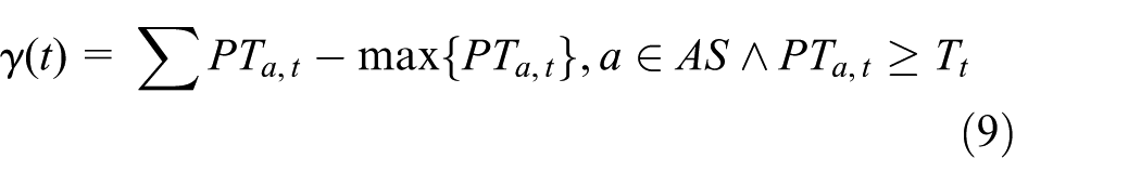
The third important criterion in RNP is calculating the amount of collision that occurs between the available efficient antennas. Collision occurs when more than one antenna interrogate the same tag, and so when the tag starts to transmit backscatter signals after receiving the induction signals from more than one antenna, these received power signals result in an interference within the network. The interference (ITF) of the network is calculated as follows

ITF = \sum_{t \in TS} γ (t)

(8)

γ (t) = \sum P T_{a, t} - max {P T_{a, t}}, a \in AS \land P T_{a, t} \geq T_{t}

(9)

The sum of the transmitted power

The transmitted power of each antenna is directly related to the interrogation range, and so by reducing the amount of transmitted power, a decrease in the coverage of the network can occur. This has the lowest criteria in the RNP. The sum of transmitted power of the network is calculated as follows

POW = \sum_{a \in AS} P S_{a}

(10)

where PS_a is the amount of transmitted power by antennas.

Optimizing RNP

The ultimate goal of optimization here is to find the optimum number of antennas that should be deployed on the RFID network in order to achieve the maximum network coverage as well as minimum interference of antennas. In this article, three different artificial intelligent techniques are utilized to perform the optimization process: GA, PSO, and RPLN.

GA

GA is part of an evolutionary computing that is used for optimizing complex problems.^36,37

The GA operates through the following steps:³⁸

Creation of a random population (normally this population size is taken as 100);

Evaluation of the fitness function of each individual;

Reproduction or selection of the best chromosomes;

Applying crossover;

Applying mutation;

Repeat steps 2–5.

The first step involves the creation of a population of chromosomes. Each population of the chromosome is known also as an individual; this is an answer to the problem. Based on the optimization problem, each chromosome contains different parameters that need to be found and optimized; these parameters are known as the genes. It should be noted that the length of genes depends on the required precision of the various problems.³⁹

To perform the first step and create a population of answers, it is necessary to learn how to encode a chromosome. There are different types of encoding which can be chosen depending on the problem’s structure. This can be a string of real numbers or binary bit string.⁴⁰

Chromosomes in binary encoding are strings, which are made of 0s and 1s; this kind of encoding is less complicated than the other methods and is normally used as a routine methodology.

The binary encoding makes use of exciting problem to define the position of the antennas and their status, that is, whether it is “on/off” or “0/1” in each chromosome.

The workspace is defined in terms of the x–y coordinate system, and so the position of each antenna can be defined as (x_r,y_r) in the workspace. The characteristics of these chromosomes depend on the length, width, and segment number of the workspace (see Figure 5).

Figure 5.

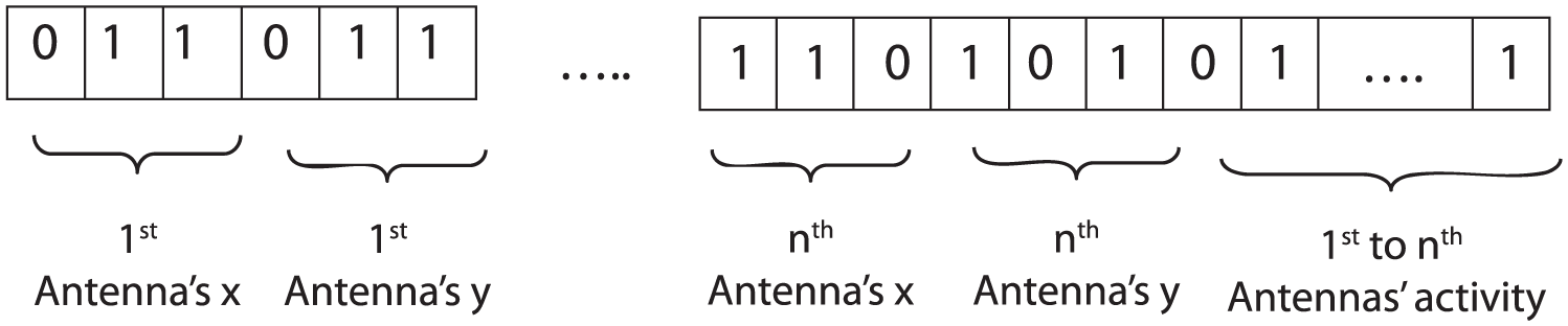
Encoding a chromosome.

The next step requires the evaluation of these individuals f(x_i). The number of antennas, coverage, and ITF should be calculated based on the position and activity of the antennas. It should be noted that in this article RAE is used to compute number of redundant antennas N_red. To implement RAE, the following steps should be taken: the antennas in each individual population should be eliminated one by one, by converting 1 to 0, that is, in the place of activity of each antenna in each chromosome. Next, the coverage should be calculated; if the calculated coverage in each step, after elimination, in the sense that an antenna remains equal to its initial state before elimination, the antenna becomes redundant and needs to be eliminated; otherwise, the activity condition of the eliminated antenna should remain as 1. This procedure needs to be implemented for the entire antenna, and so at the end, the number of antennas N_r can be calculated by counting the number of active antennas in each chromosome.

After evaluating the whole individual’s performance, the fitness function of each individual can be calculated as follows

\begin{matrix} f (x_{i}) = & \frac{100}{1 + {(100 - COV (i))}^{2}} + \frac{100}{1 + IT F^{2} (i)} i = 1 (population size) \end{matrix}

(11)

The goal is maximizing coverage and minimizing inference of the network.

Fractional fitness function of each individual is calculated as follows⁴¹

F (x_{i}) = \frac{f (x_{i})}{\sum_{i = 1}^{n} f (x_{i})} i = 1 (number of antennas)

(12)

The third step involves using the current population to produce the next generation of the population, which will have a higher objective function. This step is called the reproduction. In this step, each chromosome is copied a number of times to the next generation; this is with respect to its fractional fitness function. To select which chromosome is the fittest, different selection types have been put forward.^41,42 In this article, a roulette wheel method is utilized to perform the selection step. The main principle is that the fittest individuals, the individuals with the greatest fitness functions, have a better chance to survive.⁴²

For this purpose, the cumulative probability of each chromosome should be calculated by computing the fractional fitness function of each individual. Then, n random probability ranging from 0 to 1 should be produced; where n indicates the population size. Then it is necessary to find where each random probability is located, and which two cumulative probabilities of chromosomes it is in between. Finally, the chromosome which has the highest cumulative probability will be selected for the new population. In summary, a roulette wheel will spin n times, and each time, a chromosome will be selected for the new population.

The next step incorporates one of the GA’s operators named the crossover. The crossover makes it possible to exchange the parts of two different chromosomes, in which the production of new chromosomes takes place. In essence, the crossover forms new chromosomes (solutions) by decomposing two different chromosomes and randomly mixing the decomposed parts. In order to know the chromosomes that will participate in crossover n, a random probability number ranging from 0 to 1 should be selected; where n is the population size. When comparing the randomly produced probability of each chromosome with the probability of the crossover, which is commonly considered to have a higher probability value (Ex. 0.7), if the generated probability is equal or less than crossover probability, then that chromosome will participate in crossover. The selected crossover point, that is, a random number in range of [1 chromosome length] for each selected chromosome will be generated; the generated number indicates the crossover point. Bits, that is, to the right of the crossover point (single-point crossover), or bits located in between the generated crossover points (two-point crossover), will be exchanged with bits of another chromosome.⁴³

The final step incorporates another genetic operator named mutation. Mutation occurs randomly in one of the genes of an individual and changes its value to prevent evolutionary dead ends from occurring. If the gene value is 0, it will be changed to 1, and if it is 1, it will be changed to 0. Mutation tool is one of the nature’s most powerful survival tools. To perform mutation, n random probability number in range of [0 1] should be generated, where n is the length of the chromosome. These randomly generated probabilities will be compared to the mutation probability, which is generally a small value and can be calculated as P_m = (chromosome length)/1000. If the generated probability is less than or equal to mutation probability, then the gene value will change as follows.⁴⁴

After mutation, the new population is generated and a repetition of steps 2–5 is done. Typically, these steps are repeated 100 times, and as the property of GA is an evolutionary technique, the final outcome will be the best outcome.

Particle swarm

Eberhart and Kennedy,⁴⁵ in 1995, while observing the swarm behavior of birds flocking and fish schooling proposed a population-based stochastic optimization technique; this is known as the PSO technique. PSO like GA starts with a population of random solutions known as particles. The algorithm continues searching for the fittest value in problem space by updating the generations. In PSO, the potential solutions fly through the problem space by following the current optimum particles. However, unlike GA, PSO has no evolution operators such as crossover and mutation.⁴⁶

The canonical form of PSO, which is utilized for the optimization of the RNP in this article, is represented below¹¹

v_{i}^{t + 1} = χ (v_{i}^{t} + c_{1} r_{1} (pbes t_{i} - x_{i}^{t}) + c_{2} r_{2} (gbes t_{i} - x_{i}^{t}))

(13)

x_{i}^{t + 1} = x_{i}^{t} + v_{i}^{t + 1}

(14)

where v_i and x_i are, respectively, represented by the velocity and position vectors of each particle. pbest_i is the previous best position vector, and gbest_i is the global best position vector. Population size is presented by i, and just like the GA, it is assumed to be 100. χ is called the constriction coefficient (here, χ = 0.8), c₁ and c₂ are the learning rates (here, c₁ = c₂ = 2), and r₁ and r₂ are the random numbers that are uniformly distributed in [0, 1].

The overall procedure of the PSO algorithm can be described in the following steps:

Randomly generate the velocities and positions of particles.

For each particle, evaluate the fitness function which is proposed in equation (11) for each particle.

If the fitness is better than particle’s previous best fitness, update and then further compare the fitness with the global best fitness that has be found so far. Then, update accordingly.

Particles update their velocities and positions according to equations (13) and (14).

Loop to step 2 until a stopping criterion is reached, and in this scenario, it is completing 100 iterations.

The RPLN

RNP can be optimized using the RPLN.^47–49 Nowadays, this technique is widely used in computer engineering, especially when the concept of random-access memory (RAM) is considered. It is referred to as RPLN because each step will be done repeatedly until the desired outcome is achieved.^50,51

A PLN consists of a node and a truth table, inputs are given as 0 or 1, and the output is in the form of 0 or 1. These numbers are obtained through a decoding function and if the answer is acceptable, the truth table will be saved; otherwise, the random value will be replaced, and the operation will start from the beginning.⁵²

In other words, the PLN optimization technique is trained and learned based on pure random searches. Figure 6 shows a schematic of the PLN. This random search algorithm is known as an A-learning rule. In pattern reorganization PLN, networks can be used using A-learning rule algorithm.^53,54

Figure 6.

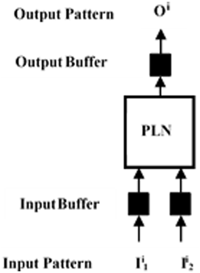
Probabilistic Logic Neuron (PLN).

The steps taken for an A-learning rule can be summarized as follows:

Encode an initial population like that discussed in GA.

For each gene in every individual (called chromosome in GA) assign a PLN with random inputs and outputs (random values).

Calculate the fitness function for each individual.

If the calculated fitness function is equal to the desired value, save the value of the inputs and outputs.

If the fitness function is not equivalent to the desired value, reset the inputs and outputs values, and then calculate the fitness function again and train the network for m times, where m is a positive non-zero integer (we assume m = 10).

If the calculated fitness function is equal to the desired value, save the value of inputs and outputs.

If the calculated fitness function is not equal to the desired value, go to the calculation for nest individual.

Repeat these steps until all the random values will be changed to the fixed values.

PLN networks can be formed in different structures, and there are no exact patterns to select which architecture should be used (see Figure 7).

Figure 7.

Example of structure of PLN network.

The structure shown in Figure 8 is used as a layer RPLN optimization structure case to optimize the RNP problem. Optimization using the RPLN is a novel technique for solving the RNP problem, and it has an advantage of simplicity in calculations and obtaining better results in less time over other computational optimization techniques.⁵⁵

Figure 8.

The Ring Probabilistic Logic Neuron, RPLN.

Results and discussion

For the purposes of this study, a 100 × 100-m² room is considered and divided into four equal segments. A total of 20 tags and 20 antennas are randomly distributed in these segments. The exact position and number of antennas are calculated through the implementation of optimization techniques (GA, PSO, and RPLN) for 100 iterations. It should be noted that the first population for all the three algorithms are considered the same, and so the results obtained are represented and compared as follows.

As seen in Figure 9, the coverage of the RNP network improves from 75% at the beginning of all GA, PSO, and RPLN optimization processes to 100%. And so, all these three algorithms can achieve the solution which gives the full network coverage; regarding to coverage of the network result that is illustrated in Figure 9, the RPLN reaches its solution faster than the other two.

Figure 9.

Calculated coverage of the network by RPLN, PSO, and GA in each iteration.

Figure 10 shows the number of calculated deployed antennas in the network, within each step of the optimization processes. This figure indicates that the number of antennas at the end of the GA optimization process is calculated as 5; however, this number is reduced to 4 in PSO and even to 2 in RPLN.

Figure 10.

Calculated number of deployed antennas in the network by RPLN, PSO, and GA in each iteration.

The combination of the results of Figures 9 and 10 can be interpreted in the following statement: since the proposed RFID network achieves full network coverage in all three optimization processes, the calculated positions of the antennas by RPLN are more efficient than the GA’s and PSO’s, because with fewer antennas, the RNP network coverage in the RPLN like GA reaches 100%.

The interference of the proposed RNP network, based on the number and position of antennas, which are calculated through GA, PSO, and RPLN optimization techniques, is shown in Figure 11. The ITF of the network at the end of the GA and PSO optimization processes, respectively, are calculated as −71.34 and −39 dBm; however, this amount through the RPLN optimization process is calculated as −23.34 dBm. Therefore, this result indicates that utilizing RPLN gives more reliable antennas positioning when compared to GA and PSO optimization techniques.

Figure 11.

Calculated ITF of the network by RPLN, PSO, and GA in each iteration.

Overall, the results indicate that utilizing the RPLN optimization technique, compared to the GA and PSO techniques, optimizes an RNP. This makes it more cost-effective and time-efficient, since the RFID network can reach full network coverage in lesser time due to fewer deployment of antennas and lesser interference on the network.

Conclusion

In this article, a pure random-based optimization technique called the RPLN has been introduced as an efficient optimization technique for dealing with a complex RNP problems. This optimization technique is capable of adjusting any number of embedded RFID antennas in the network. The simulation-based performance assessment has been performed for investigating the effectiveness of the RPLN algorithm over the GA and PSO. The simulation results show that the RPLN has superior performance over the GA and PSO. However, it should be noted that in order to prevent antenna redundancy deployment in the network, all three optimization techniques have been enhanced with an additional algorithm named the RAE. It should be observed that the RPLN technique for optimizing the RNP is more enhanced than GA and PSO as explained below:

RPLN has faster convergence speed and lesser iterations than GA and PSO.

RPLN has lesser complexity in computations than GA and PSO.

The results given by the RPLN are more precise and cost-effective.

In future studies, with an innovation in the proposed mathematical models of the RNP, it will be possible to model an RFID network that involves more criteria such as the quality of the network. A valuable future study would involve the utilization of more optimization techniques for static and dynamic networks to generate RFID networks.

Footnotes

Acknowledgements

The authors would like to thank the anonymous reviewers for their valuable comments and feedbacks to enhance the quality of the paper.

Academic Editor: Shengyong Chen

Declaration of conflicting interests

The author(s) declared no potential conflicts of interest with respect to the research, authorship, and/or publication of this article.

Funding

The author(s) received no financial support for the research, authorship, and/or publication of this article.

References

Barenji

Hashemipour

A frameworks for structural modelling of an RFID-enabled intelligent distributed manufacturing control system. S Afr J Ind Eng 2014; 25: 48–66.

Guédon

Wauben

de Korne

. A RFID specific participatory design approach to support design and implementation of real-time location systems in the operating room. J Med Syst 2015; 39: 1–10.

Barenji

AV.

An RFID-based distributed control system for flexible manufacturing system. Eastern Mediterranean University (EMU)-Doğu Akdeniz Üniversitesi (DAÜ), 2013, http://i-rep.emu.edu.tr:8080/jspui/bitstream/11129/1360/1/BarenjiAli.pdf

Guo

Ngai

Yang

. An RFID-based intelligent decision support system architecture for production monitoring and scheduling in a distributed manufacturing environment. Int J Prod Econ 2015; 159: 16–28.

Barenji

Hashemipour

Flexible testing platform for employment of RFID-enabled multi-agent system on flexible assembly line. Adv Eng Softw 2016; 91: 1–11.

Barenji

Hashemipour

A multi-agent RFID-enabled distributed control system for a flexible manufacturing shop. Int J Adv Manuf Tech 2014; 71: 1773–1791.

Chen

Zhu

. RFID network planning using a multi-swarm optimizer. J Netw Comput Appl 2011; 34: 888–901.

Chen

. Hierarchical artificial bee colony algorithm for RFID network planning optimization. Sci World J 2014; 2014: Article ID 941532 (21 pp.).

Zhu

. Cooperative artificial bee colony algorithm for multi-objective RFID network planning. J Netw Comput Appl 2014; 42: 143–162.

10.

Guan

Liu

Yang

. Genetic approach for network planning in the RFID systems. In: 2006 ISDA’06 sixth international conference on intelligent systems design and applications, Jinan, China, 16–18 October 2006, pp.567–572. New York: IEEE.

11.

Yang

Xia

. A RFID network planning method based on genetic algorithm. In: 2009 NSWCTC’09 international conference on networks security, wireless communications and trusted computing, Wuhan, Hubei, 25–26 April 2009, pp.534–537. New York: IEEE.

12.

Zhou

Ranasinghe

DC.

A novel approach for addressing wandering off elderly using low cost passive RFID tags. In: Stojmenovic

Cheng

Guo

(eds) Mobile and ubiquitous systems: computing, networking, and services. Berlin: Springer, 2013, pp.330–343.

13.

Gong

Y-J

Shen

Zhang

. Optimizing RFID network planning by using a particle swarm optimization algorithm with redundant reader elimination. IEEE T Ind Inform 2012; 8: 900–912.

14.

Spekman

Sweeney

PJ.

RFID: from concept to implementation. Int J Phys Distrib 2006; 36: 736–754.

15.

Optimal scheduling-based RFID reader-to-reader collision avoidance method using artificial immune system. Appl Soft Comput 2013; 13: 2557–2568.

16.

Kuo

Shieh

Zhang

. The application of an artificial immune system-based back-propagation neural network with feature selection to an RFID positioning system. Robot Cim: Int Manuf 2013; 29: 431–438.

17.

Garcia-Valverde

Garcia-Sola

Hagras

. A fuzzy logic-based system for indoor localization using WiFi in ambient intelligent environments. IEEE T Fuzzy Syst 2013; 21: 702–718.

18.

Botero

Chaouchi

. RFID network topology design based on genetic algorithms. In: 2011 IEEE international conference on RFID-technologies and applications (RFID-TA), Sitges, 15–16 September 2011, pp.300–305. New York: IEEE.

19.

Bhattacharya

Roy

UK.

Optimal placement of readers in an RFID network using particle swarm optimization. Int J Comput Netw Commun 2010; 2: 225–234.

20.

Chen

Zhu

. Multiobjective RFID network optimization using multiobjective evolutionary and swarm intelligence approaches. Math Probl Eng 2014; 2014: Article ID 961412 (13 pp.).

21.

Feng

. Optimal RFID networks planning using a hybrid evolutionary algorithm and swarm intelligence with multi-community population structure. In: 2012 14th international conference on advanced communication technology (ICACT), PyeongChang, South Korea, 19–22 February 2012, pp.1063–1068. New York: IEEE.

22.

Nawawi

Hasnan

Ahmad Bareduan

Correlation between RFID network planning (RNP) parameters and particle swarm optimization (PSO) solutions. Appl Mech Mater 2014; 465–466: 1245–1249.

23.

A fuzzy k-coverage approach for RFID network planning using plant growth simulation algorithm. J Netw Comput Appl 2014; 39: 280–291.

24.

Tuyls

Batina

. RFID-tags for anti-counterfeiting. In: Pointcheval

(ed.) Topics in cryptology–CT-RSA 2006. Berlin: Springer, 2006, pp.115–131.

25.

Chawla

DS.

An overview of passive RFID. IEEE Commun Mag 2007; 45: 11–17.

26.

Zhu

Cao

. Fault-tolerant RFID reader localization based on passive RFID tags. IEEE T Parall Distr 2014; 25: 2065–2076.

27.

Oztekin

Pajouh

. An RFID network design methodology for asset tracking in healthcare. Decis Support Syst 2010; 49: 100–109.

28.

Shaw

JA.

Radiometry and the Friis transmission equation. Am J Phys 2013; 81: 33–37.

29.

Azad

Jing

Wang

YE.

Link budget and capacity performance of inductively coupled resonant loops. IEEE T Antenn Propag 2012; 60: 2453–2461.

30.

Chae

H-J

Salajegheh

Yeager

. Maximalist cryptography and computation on the WISP UHF RFID tag. In: Smith

(ed.) Wirelessly powered sensor networks and computational RFID. Berlin: Springer, 2013, pp.175–187.

31.

Tao

Huang

. SA-PSO based optimizing reader deployment in large-scale RFID Systems. J Netw Comput Appl 2015; 52: 90–100.

32.

Abkenar

SMS

Stanley

Miller

. Evaluation of genetic algorithms using discrete and continuous methods for pump optimization of water distribution systems. Sustain Comput: Inform Syst 2015; 8: 18–23.

33.

Alsalihy

WAA

Askar

. Enhancement of redundant reader elimination by using hybrid algorithm in RFID systems. Wireless Pers Commun 2013; 72: 1139–1156.

34.

Dimitriou

Siachalou

Bletsas

. Automated RFID network planning with site-specific stochastic modeling and particle Swarm Optimization. In: 2014 IEEE RFID technology and applications conference (RFID-TA), Tampere, 8–9 September 2014, pp.44–49. New York: IEEE.

35.

Hsu

C-H

Zhang

Yang

C-T

. An efficient method for optimizing RFID reader deployment and energy saving. arXiv preprint arXiv:13053338, 2013, http://arxiv.org/abs/1305.3338

36.

Dias

Rocha

Ferreira

. A genetic algorithm with neural network fitness function evaluation for IMRT beam angle optimization. Cent Europ J Oper Re 2014; 22: 431–455.

37.

Martínez-Soto

Castillo

Castro

. Genetic algorithm optimization for type-2 non-singleton fuzzy logic controllers. In: Castillo

Melin

Pedrycz

. (eds) Recent advances on hybrid approaches for designing intelligent systems. Berlin: Springer, 2014, pp.3–18.

38.

Ahn

Ramakrishna

RS.

A genetic algorithm for shortest path routing problem and the sizing of populations. IEEE T Evolut Comput 2002; 6: 566–579.

39.

Jose Filho

Treleaven

Alippi

Genetic-algorithm programming environments. Computer 1994; 27: 28–43.

40.

Dezani

Bassi

Marranghello

. Optimizing urban traffic flow using genetic algorithm with Petri net analysis as fitness function. Neurocomputing 2014; 124: 162–167.

41.

Man

K-F

Tang

Kwong

Genetic algorithms: concepts and designs. Berlin: Springer, 2012.

42.

Semenkin

Semenkina

Self-configuring genetic algorithm with modified uniform crossover operator. In: Tan

Shi

(eds) Advances in swarm intelligence. Berlin: Springer, 2012, pp.414–421.

43.

Michalewicz

Genetic algorithms + data structures = evolution programs. Berlin: Springer, 2013.

44.

Chen

C-H

Kuo

C-M

Hsieh

S-H

. RETRACTED: highly efficient very-large-scale integration (VLSI) implementation of probabilistic neural network image interpolator. J Vib Control 2014; 20: 218–224.

45.

Eberhart

Kennedy

A new optimizer using particle swarm theory. Proceedings of the sixth international symposium on micro machine and human science, Nagoya, Japan, 4–6 October 1995, pp.39–43. New York: IEEE.

46.

Khare

Rangnekar

A review of particle swarm optimization and its applications in solar photovoltaic system. Appl Soft Comput 2013; 13: 2997–3006.

47.

Menhaj

Seifipour

Function optimization by RPLNN. In: 2002 IJCNN’02 proceedings of the 2002 international joint conference on neural networks, Honolulu, HI, 12–17 May 2002, pp.1522–1527. New York: IEEE.

48.

Seyfipour

Menhaj

Nik

RS.

A new optimization method by ring probabilistic logic neural networks. Amirkabir J Sci Technol 2003; 14: 43–57.

49.

Wasserman

PD.

Advanced methods in neural computing. Hoboken, NJ: John Wiley & Sons, 1993.

50.

Ramsey

Rumelhart

Stich

SP.

Philosophy and connectionist theory. Hove: Psychology Press, 2013.

51.

Thompson

Hardware Evolution: automatic design of electronic circuits in reconfigurable hardware by artificial evolution. Berlin: Springer, 2012.

52.

Austin

. A review of RAM based neural networks. In: Proceedings of the fourth international conference on microelectronics for neural networks and fuzzy systems, Turin, 26–28 September 1994, pp.58–66. New York: IEEE.

53.

Aleksander

De Gregorio

França

FMG

. A brief introduction to Weightless Neural Systems. In: ESANN, 2009, http://ftp.bstu.by/ai/To-dom/My_research/Papers-3/Intention/BDI-model/NN/es2009-6.pdf

54.

Berthold

Diamond

Constructive training of probabilistic neural networks. Neurocomputing 1998; 19: 167–183.

55.

Wang

C-H

Tsai

S-W.

Optimizing bi-objective imperfect preventive maintenance model for series-parallel system using established hybrid genetic algorithm. J Intell Manuf 2014; 25: 603–616.

Optimizing radio frequency identification network planning through ring probabilistic logic neurons

Abstract

Keywords

Introduction

RNP

Mathematical modeling of RFID network planning

Coverage

The number of antennas

RAE

Interference

The sum of the transmitted power

Optimizing RNP

GA

Particle swarm

The RPLN

Results and discussion

Conclusion

Footnotes

Acknowledgements

Declaration of conflicting interests

Funding

References