
Abstract
Nanotechnology is a very important field in science and technology, and research projects in this domain attract considerable funding. The existing research works in nanotechnology deal with chemical, physical, and biological issues or a combination of these fields, but very small number of works has been undertaken on mathematical modeling. Mathematical models can greatly reduce the time involved in experimentation, which in turn reduces the research cost. In this article, we consider the mathematical modeling of the motion of nanoparticles in a viscous flow inside straight tube. Illustrative simulations of the model are provided.
Introduction
In this article, we are working on the modeling and simulations of some important phenomena raised in biotechnology and medicine at the nanoscale. We focus on the modeling and simulations of the motion of nanoparticles in artificial straight microtubes. The case of human capillaries (see Figure 1) and more complex artificial capillaries will be the second phase of our research work (forthcoming papers).

Examples of human capillaries.
Our motivations come from the great impact of nanotechnology and biotechnology on pharmacology for improving performance of many drugs and allowing the use of new drugs and new therapies. Also, nanoparticles can be manufactured and used as drug delivery systems to (1) deliver drugs specifically at places where diseased cells are, and optimally control drug release rates—preprogrammed, self-regulated, and remotely controlled delivery vehicles; (2) locate diseased cells or tumoral masses and estimate the state of the disease; and (3) carry diagnostic agents (fluorescence molecules) to enhance imaging.
Based on these motivations, we started working on the following research direction: modeling and simulations of the motion of nanoparticles in straight tubes (the case of general shapes will be the subject of forthcoming papers) and taking into account all the interactions between them and with walls and obstacles. On this direction, we obtained satisfactory numerical simulations in the simplest prototype of straight circular capillaries (see Figure 2).

Straight circular capillaries.
The main task of the mathematical model used in our analysis is the non-overlapping of the nanoparticles and the obstacles inside the channel during the simulation. In a forthcoming paper, we will treat more complex situations in which we will take into account all the possible forces governing the flow inside the micro-channel (for instance, the forces exerted by the blood (or liquid) stream, gravitation, and electromagnetic interactions) and all the possible forces between nanoparticles and surfaces (for instance, Van der Waals, steric-polymer forces, electrostatic interaction (repulsive and attractive), hemodynamic forces, buoyancy, etc). Also, the shape of the channel will be taken in a more general form, that is, the walls will be a function
The present work is organized as follows. The section “Notation” is stated in Appendix I and it contains the notation that will be used throughout the paper. In section “Non-overlapping algorithm,” we build and analyze the algorithm that will be used to ensure the non-overlapping of the nanoparticles. Section “Dynamical system of the motion of nanoparticles” is devoted to derive the dynamical system governing the motion of nanoparticles inside the micro-channel. In section “Illustrative simulation,” we present our satisfactory numerical simulations.
Non-overlapping algorithm
In this section, we present a numerical scheme that can be used to handle contacts between rigid disks. This numerical scheme will be our main powerful tool to simulate without overlapping the motion of nanoparticles. This algorithm has been introduced by Maury 1 for studying inelastic collision problems and used by Maury and Venel 2 for the modeling of microscopic crowd motion. For another application of this algorithm to other practical problems (to obstacle avoidance of mobile robots), we refer the reader to Hedjar and Bounkhel. 3
Consider N nanoparticles identified to inelastic disks with different radii
We consider the configuration vector

where

Here,

Taking the real velocity at that time

and hence
Let
Assume that

where

The numerical scheme (4) can be seen geometrically as
Remark 1
The main characterizations of the above algorithm are as follows: as explained before, the first one is the non-overlapping between the disks, which is ensured by the setup of the algorithm. However, the second characterization, which is the most requested in numerical analysis, is the continuity of the trajectory of the nanoparticles generated by the algorithm. This property of smoothness has been proved by Maury and Venel 2 (see also section 3 in Hedjar and Bounkhel 3 ).
Dynamical system of the motion of nanoparticles
In this section, we are going to build the system of differential equations of the motion of nanoparticles inside a straight tube.
Consider the motion of N nanoparticles in a viscous flow inside a tube of width a and length l and bounded by two horizontal walls as shown in Figure 4. Let

Nanoparticles inside a straight tube.
The trajectory of each nanoparticle is governed by the forces exerted by the flow (blood stream) and the gravitation. Forces acting on nanoparticles include hemodynamic forces, buoyancy, Van der Waals interactions between nanoparticles each-to-other and between nanoparticles and walls.
To derive the equations describing the motion on the x-axis and on the z-axis, we apply (as suggested by Zhao et al. 4 ) the balance principle of forces acting on the nanoparticles. 5 The balance of forces acting on the nanoparticles requires, for each nanoparticle i, a system of two equations on the x-axis and the z-axis. So, on the z-axis, we have, for any nanoparticle i, the following equation
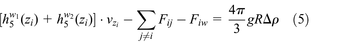
where

where

where

where

Motion of 500 nanoparticles inside a straight microtube.
On x-axis, we have, for any nanoparticle i, the following equation

where S is the shear rate of the flow and the functions

and
Equations (5) and (7) are, respectively, the force balance in the x- and z-directions. In these equations,

Remark 2
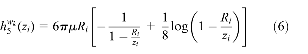
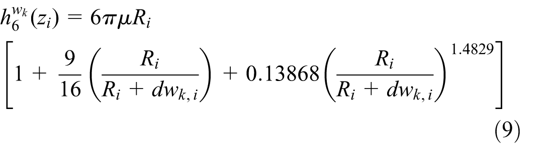
For a spherical particle, the hydrodynamic resistance function
The approximations of the hemodynamic resistant function
The two equations for the force balance contain two unknowns, namely, the two velocity components
The function
Illustrative simulation
In our simulations, we assume that
Discussion
The first image in Figure 4 shows the initial situation (taken randomly) of the nanoparticles inside the microtube with diameter
Conclusion
In this work, we considered the simple situation (straight tube and only van der Waals’ interaction) in order to setup an approach to produce a realistic numerical simulation for a huge number of moving nanoparticles. Our next task which seems to be doable, due to the flexibility of our iterative scheme, is to insert all the possible forces acting on the nanoparticles, some existing obstacles (fixed or moving), and also the general form of the function defining the shape of the tube.
Footnotes
Appendix 1
Academic Editor: Xiaotun Qiu
Declaration of conflicting interests
The author(s) declared no potential conflicts of interest with respect to the research, authorship, and/or publication of this article
Funding
The author(s) disclosed receipt of the following financial support for the research, authorship, and/or publication of this article: The author would like to extend his sincere appreciations to the Deanship of Scientific Research at King Saud University for funding this Research Group (No. RGP-024).