MARIN rudder mathematical model

Abstract

This paper presents the mathematical model used in MARIN’s time domain software to describe the hydrodynamic loads excited by a rudder. The paper provides a detailed description of the mathematical model and its theory, along with highlighting the novel features that have been added to extend the model to four quadrants operations. Furthermore, the paper compares the mathematical model with experiments, showcasing the model’s capabilities and shortcomings. For this comparison, a spade rudder behind the KRISO Container Ship with and without a propeller upstream has been used as a case study to illustrate how the model performs in practice.

1. Introduction

When simulating a manoeuvring floating body, mathematical models are used to calculate the hydrodynamic loads that determine its motion. A rudder plays a significant role in these hydrodynamic loads.

The main contribution of this paper is to publish the latest version (February 2024) of the mathematical rudder model for the MARIN simulation platform XMF.1

¹

The Extensible Modelling Framework (XMF) is a C++ software toolkit on which all MARIN’s time domain simulation software developments are based. Dynamic content libraries provide XMF with domain specific features to simulate hydrodynamic aspects. The rudder model is part of these libraries.

Over the years, various mathematical models for rudders have been developed, drawing from the existing literature. The rudder model proposed by the Japanese research group named Maneuvering Mathematical Modeling Group (MMG) introduced a different way of modelling: the rudder model is not a polynomial expression fitting forces from captive experiments (also known as Abkowitz’s model [1] or “whole ship” model), but a model based on physical principles dedicated to the rudder (also known as “modular” model).

The MMG model, starting from the early publications (e.g. [10,15], or [12]) up to the more recent ones (e.g. for instance [20]) showed during the years how to define a new way of modelling, combining physical principles with observations and measurements from experimental data. Many models were derived using this new way, as for instance in [3] and [11].

The advantage of the models in [10] and [11] is that they can be used in the initial design stage, because only main particulars are needed.

At MARIN, two main “modular” rudder models were developed: one was developed for the simulation program FREDYN (dynamic behaviour of a steered ship subjected to waves and wind) and published in [9]; the second was developed for the simulation program SURSIM (calm water manoeuvring with displacement ships) and published in [8]. These publications present the first version of the models, but further developments were not published.

All these models provide a standard method for ship manoeuvring predictions, including models for propeller and hull. Therefore the MMG model, and the models following it, are wider than “just” a rudder model. However, this paper focuses on the rudder “sub-model” (and the interactions with propeller and hull).

Although these rudder “sub-models” have a common theoretical background, they describe the interactions with hull and propeller differently and they have different inherent empirical coefficients.

All these models have many advantages, from a sound physical meaning up to the easy applicability, and proved to be quite accurate for specific applications. These applications consist of calm water manoeuvring predictions in 3 (surge, sway, yaw) or 4 (including roll) degrees of freedom, with particular attention to the standard IMO manoeuvres such as zig-zag and turning circle manoeuvres. How accurate these models are for different applications is not clear (even though the model in [9] is meant for the manoeuvrability of frigates in waves).

What is clear is that they might be limited. In fact, manoeuvring studies require more and more to look at broader applications, including:

Scenarios in the four quadrants of operation, therefore with combinations of positive or negative ship’s speed and positive or negative propeller revolutions.

Designs with rudders not aligned with the propellers, therefore only partially covered by the propeller outflow.

Situations with all kinds of inflow to the rudder, including situations with a cross flow, like when drifting in beam waves or when turning on the spot.

Operations with rudder angles above the typical maximum angle of 35 degrees, like for instance when dealing with inland ships.

Therefore, there is a need for more flexible and robust rudder mathematical models.

Section 2 describes the limitations from the models in the literature. Section 3 presents the MARIN mathematical model, including a thorough theoretical description. Section 4 shows the application of the mathematical model, including a comparison to experimental results to validate the model. Section 5 highlights the novel features of the model, including a critical and detailed evaluation against previous models from MARIN and the literature. Conclusions are presented in Section 6.

Appendix A presents the case study. Appendix B lists the empirical coefficients within the mathematical model presented here used in the case study. Appendix C provides a list of symbols (of coefficients and parameters) used in this paper, including a comparison and link to the literature.

2. Review of the limitations in the literature

The following limitations in the models from the literature are found:

The MMG model [20] and the model in [11] describe effectively the longitudinal inflow velocity component to the rudder, including the propeller slip stream (considering also how much of the rudder is hit by the slip stream). However, the models use propeller open water characteristics (advance and thrust coefficients) that cannot be defined in the four quadrants of operation. This will limit the use of the model (as already pointed out in [3]), being undefined when simulating astern manoeuvres or even leading to a mathematical singularity for instance when simulating manoeuvres with a blocked propeller. The MARIN model in [9] does not describe the flow increment due to the propeller. The other MARIN model in [8] does not lead to mathematical singularities, but does not take directly into account how much of the rudder is hit by the slip stream.

The MMG model [20] and the model in [11] consider how much of the rudder is hit by the slip stream (“rudder coverage”), using the ratio between propeller diameter and rudder span. In case of a rudder not aligned with the propeller transversal or vertical position, this ratio can overestimate the rudder coverage, leading to inaccurate estimation of the inflow velocity. The MARIN models in [9] and [8] do not consider the rudder coverage.

The MMG model [20] and the MARIN model in [9] simplify the rudder drag. In [20], an empirical factor is considered to define the rudder resistance (parasitic drag), to include this effect at least in the longitudinal component of the force in a ship-fixed coordinate system (but not in the transversal one). This can be inaccurate at high drift angles, that can occur when manoeuvring in waves or in an harbour, where the cross flow drag is present.

The MMG model, the MARIN models in [9] and [8], and the models in [3] and [11] include a flow straightening coefficient, describing how the actual inflow angle to the rudder differs from the geometrical one due to the presence of hull and propeller. The factor was introduced in [15] and then developed further in [12] and [20]. Even though [15] indicates a changing tendency of this coefficient with increasing drift angle, this effect is not included in these models. This can be inaccurate at high drift angles where the presence of hull and propeller is likely less dominant, since the rudder (especially the outer rudder in case of multiple rudders) is less in the “shadow” of hull and propeller (effecting the wake fraction, in addition to the flow straightening coefficient).

The MMG model, the MARIN models in [9] and [8], and the models in [3] and [11] consider only the rudder normal force (see Fig. 1) and computes the longitudinal and transversal components of the effective rudder force by multiplying the normal force respectively to the sine and cosine of the rudder angle. This means that the stall angle is assumed to be always at 45 degrees. This is not always true. Therefore this model could be inaccurate at the rudder angles close to or higher than the “real” stall angle.

3. Mathematical model

The rudder mathematical model describes the flow around the rudder, averaging velocity and force components in a single point of application. The model is defined by the dimensions (see Fig. 2), location, and stock inclination angle in the y-z plane. The model includes the interactions with the hull and a propeller (when present). These interactions consist for instance of the effect of an accelerated inflow when positioned in a propeller slip stream, or the effect of a straightened inflow due to the presence of the hull. The mathematical model is based on lifting line and axial momentum (actuator disc) theory, with the implementation of empirical coefficients based on wind tunnel and towing tank model tests.

As described in [14], the purpose of a movable device that steers a ship, such as a rudder, is either to maintain the ship on a particular course or to manoeuvre. This force arises from the difference in the average pressure of the fluid flowing through the rudder surface, as sketched in Fig. 1.

Fig. 1.

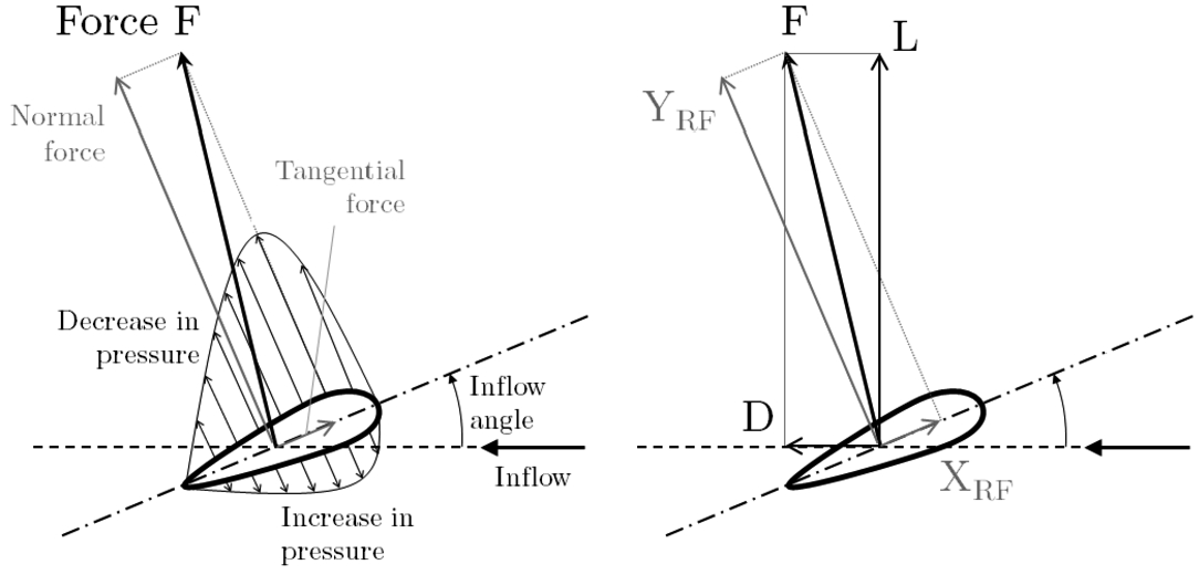
Sketch of a rudder force due to an inflow.

Fig. 2.

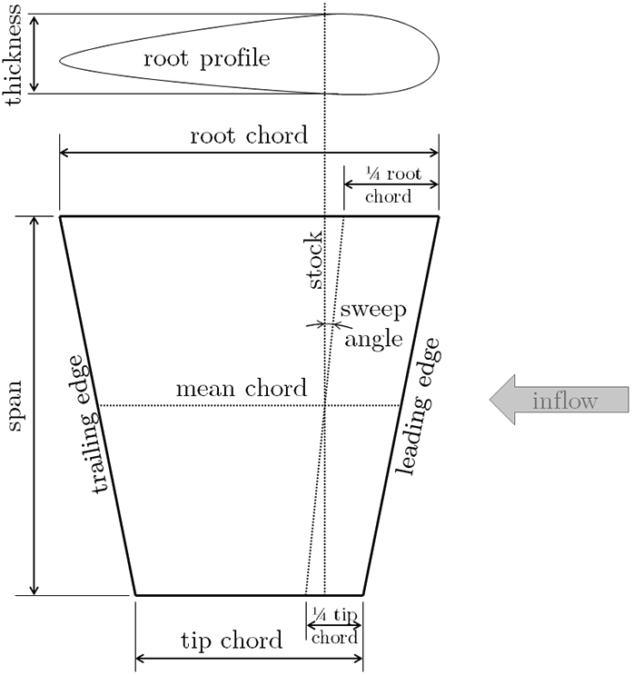
Sketch of a rudder defining the main geometric characteristics.

The force is usually resolved into a lift and a drag component, respectively perpendicular and parallel to the undisturbed inflow fluid stream, and expressed in terms of dimensionless coefficients for a given inflow angle, which is the angle between the chord and the flow, as $$\begin{array}{}\text{(1)}& {\mathit{C}}_{\mathit{L}}={\displaystyle \frac{\mathit{L}}{0.5·\mathit{\rho }·{\mathit{A}}_{\mathit{R}}·{\mathit{V}}_{\mathit{I}}^2}}\mathrm{,}\text{(2)}& {\mathit{C}}_{\mathit{D}}={\displaystyle \frac{\mathit{D}}{0.5·\mathit{\rho }·{\mathit{A}}_{\mathit{R}}·{\mathit{V}}_{\mathit{I}}^2}}\mathrm{,}\end{array}$$ where ρ is the fluid density, ${\mathit{A}}_{\mathit{R}}$ is the lateral projected area of the rudder, and ${\mathit{V}}_{\mathit{I}}$ is the inflow velocity (seen as the velocity of the rudder with respect to the fluid). This inflow velocity is computed as ${\mathit{V}}_{\mathit{I}}=\sqrt{{\mathit{u}}_{\mathit{I}}^2+{\mathit{v}}_{\mathit{I}}^2}$ , with ${\mathit{u}}_{\mathit{I}}$ and ${\mathit{v}}_{\mathit{I}}$ respectively the longitudinal and transversal components of the velocity in a ship-fixed coordinate system (i.e. a coordinate system that follows the position of the ship and rotates with the yaw, pitch and roll rotations of the ship).

The rudder force can be expressed in components in a rudder-fixed (with the subscript “RF” in Fig. 1) or a ship-fixed coordinate system (coinciding with the lift and drag in Fig. 1 assuming the rudder aligned with the center line of the ship).

Rudder effectiveness relies on the amount of force for manoeuvring. Rudder efficiency relates to the lift to drag ratio. Lift and drag depend on the geometry, and the direction and velocity of the inflow that, in turn, affects the (effective) inflow angle.

3.1. Geometry: Rudder aspect ratio

For typical rudders, the aspect ratio has the most significant influence on the lift and drag [19]. The aspect ratio can be distinguished between geometric ${\mathit{AR}}_{\mathit{G}}$ and effective ${\mathit{AR}}_{\mathit{E}}$ . The geometric aspect ratio is the ratio between the $\mathit{height}$ (or span) and the $\mathit{meanChord}$ (or width) of the movable part of the rudder or, the ratio between the square of the span and the rudder lateral projected area ${\mathit{A}}_{\mathit{R}}=\mathit{height}·\mathit{meanChord}$ . The effective aspect ratio is function of the geometric aspect ratio and takes into account an increase or decrease by a coefficient $\mathit{car}$ of the geometric aspect ratio, as $$\begin{array}{}\text{(3)}& {\mathit{AR}}_{\mathit{E}}=\mathit{car}·{\mathit{AR}}_{\mathit{G}}=\mathit{car}·{\displaystyle \frac{\mathit{height}}{\mathit{meanChord}}}=\mathit{car}·{\displaystyle \frac{{\mathit{height}}^2}{{\mathit{A}}_{\mathit{R}}}}\mathrm{,}\end{array}$$ with the coefficient $\mathit{car}$ as a theoretical maximum of 2 for a foil against a large flat plate. For a two-dimensional foil, $\mathit{car}$ is infinite.

Free surface effects on the surface piercing are taken into account by clipping the rudder height at the instantaneous water level (including waves when specified). The wetted part is used to determine the clipped aspect ratio, used in place of the geometric one.

3.2. Lift

A lifting surface of infinite aspect ratio has the same flow over all sections and the flow is said to be two-dimensional (in practice, this can be seen as a rudder with infinitely large plates at the top and bottom). For finite aspect ratio, flow occurs over the ends from high pressure to low pressure sides and the flow is said to be three-dimensional. A gap at the root of the lifting surface, the shape of the adjacent hull, and how these two characteristics change depending on the rudder angle are important features that lead to a decrease of the effective aspect ratio, as shown in [14].

Using the theoretical two-dimensional lift curve slope which is $2·\mathit{\pi }$ , the theoretical three-dimensional lift curve slope ${[{\mathit{dC}}_{\mathit{L}}\mathrm{/}\mathit{d}\mathit{\alpha }]}_{\mathit{\alpha }=0}$ at an inflow angle α of zero degrees can be expressed as $$\begin{array}{}\text{(4)}& {[{\mathit{dC}}_{\mathit{L}}\mathrm{/}\mathit{d}\mathit{\alpha }]}_{\mathit{\alpha }=0}={\displaystyle \frac{2·\mathit{\pi }}{1+2\mathrm{/}{\mathit{AR}}_{\mathit{E}}}}={\displaystyle \frac{2·\mathit{\pi }·{\mathit{AR}}_{\mathit{E}}}{{\mathit{AR}}_{\mathit{E}}+2}}.\end{array}$$

This theoretical three-dimensional lift curve slope tends to give values at a particular aspect ratio that are higher than the ones derived from experiments. Therefore, empirical coefficients with different values in the dividend and divisor are introduced. Empirical coefficients can also be used in order to correct the assumption that the lift depends only on the effective aspect ratio. The effect of other geometric characteristics such as the taper ratio (ratio between the tip and root chord), section shape, thickness, sweep of quarter chord, or tip shape can be taken into account in these empirical coefficients. As shown in the literature [14], different rudder types can be described by different lift slopes.

The lift curve slope coefficient is then calculated as $$\begin{array}{}\text{(5)}& {[{\mathit{dC}}_{\mathit{L}}\mathrm{/}\mathit{d}\mathit{\alpha }]}_{\mathit{\alpha }=0}={\displaystyle \frac{\mathit{clslope}\text{\_}\mathit{num}·\mathit{\pi }·{\mathit{AR}}_{\mathit{E}}}{{\mathit{AR}}_{\mathit{E}}+\mathit{clslope}\text{\_}\mathit{denom}}}.\end{array}$$

Typical empirical coefficients are $\mathit{clslope}\text{\_}\mathit{num}=1.95$ and $\mathit{clslope}\text{\_}\mathit{denom}=2.25$ , based on theoretical and empirical background (see [4], or Fig. 3 in [12]).

The lift coefficient is then calculated as the lift curve slope times (a function of) the effective inflow angle ${\mathit{\delta }}_{\mathit{eff}}$ as $$\begin{array}{}\text{(6)}& {\mathit{C}}_{\mathit{L}}={[{\mathit{dC}}_{\mathit{L}}\mathrm{/}\mathit{d}{\mathit{\delta }}_{\mathit{eff}}]}_{{\mathit{\delta }}_{\mathit{eff}}=0}·cos{\mathrm{(}{\mathit{\delta }}_{\mathit{eff}}\mathrm{)}}^{\mathit{cstall}}·sin\mathrm{(}{\mathit{\delta }}_{\mathit{eff}}\mathrm{)}.\end{array}$$

The sine and cosine functions are used in order to take into account the stall behaviour which is discussed in Section 3.3.

The effective inflow angle ${\mathit{\delta }}_{\mathit{eff}}$ is function of the rudder angle δ and the inflow angle α as discussed in Section 3.5.

3.3. Stall

As described in [14] and [2], at small angles, the flow around the rudder surface is smooth and attached to both the high and low-pressure side. The points of separation of the flow are near the trailing edge. As the inflow angle increases, the flow detaches from the low-pressure side, starting from the trailing edge. As the inflow angle increases even more, there is a further increase in pressure (is less negative) and a further rapid movement forwards of the separation point. This will continue until the whole surface on low-pressure side is in the separation zone.

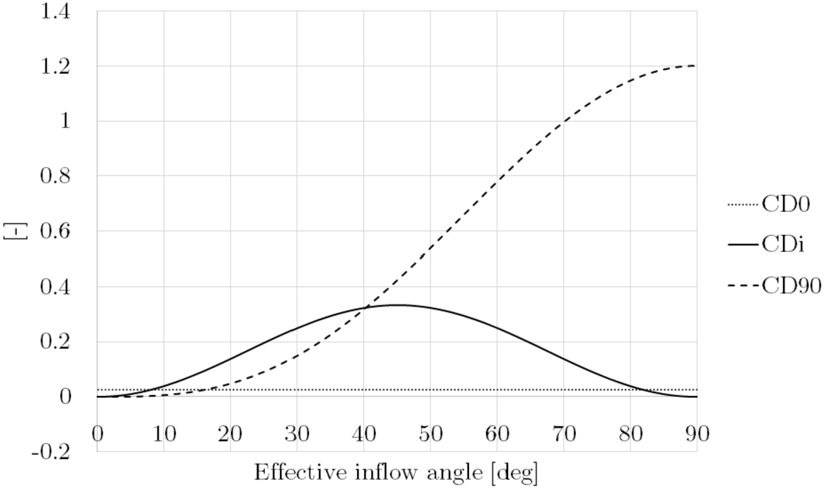
This process is called stall and it leads to a loss of lift and change in drag, as depicted in Fig. 3.

Fig. 3.

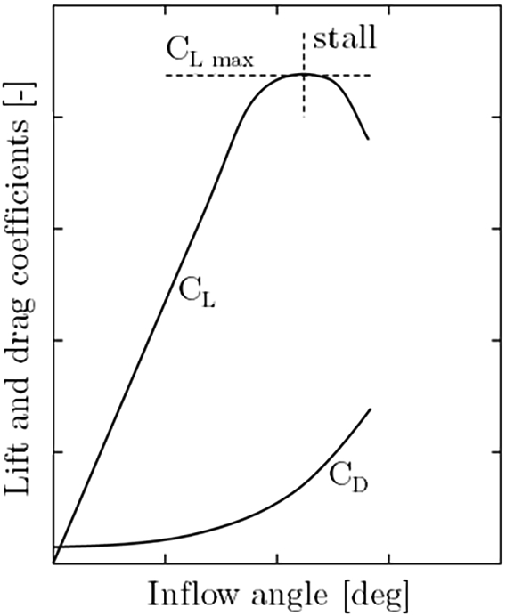
Lift and drag curves.

It should be noted that there is not a complete loss of lift after stall, as the surface is still driving off its lower pressure surface. Moreover, especially for marine rudders behind a propeller, the stall will happen gradually on the surface. For these reasons and based on model experiments, the stall angle can be taken into account directly in the lift equation, using a sine and cosine function (see Equation (6)).

The coefficient $\mathit{cstall}$ defines the stall angle. In fact, given a stall angle, $\mathit{cstall}$ is computed as $$\begin{array}{}\text{(7)}& \mathit{cstall}={\displaystyle \frac{1}{tan{\mathrm{(}\mathit{stallAngle}\mathrm{)}}^2}}.\end{array}$$

A $\mathit{cstall}$ of 1 corresponds to a stall angle of 45 degrees. A $\mathit{cstall}$ of 0.333 and 3 correspond respectively to a stall angle of 60 and 30 degrees. Wind tunnel tests [19] shows that the lower the effective aspect ratio, the higher the stall angle.

3.4. Drag

With infinite span, fluid motions are two-dimensional and perpendicular to the span. The lift and drag are associated with the shape of the section rather than the shape of the whole surface.

With finite span or finite aspect ratio, fluid motions also take place in the span wise direction and are three-dimensional [2,14]. When lift is produced, there is a difference in the fluid pressure between the upper and lower surface. Fluid pressure must equalise at the edges of a finite span surface, since a pressure difference can only be sustained by the surface itself. The resulting span wise pressure gradients force the flow on one side out towards the tip and root and on the other towards the centre of the span. The flow leaving the trailing edge forms a surface of discontinuity and a sheet of vortices is set up. This sheet of vortices is unstable and rolls up into a pair of concentrated trailing vortices close to the tip and root (see Fig. 4).

Fig. 4.

Sheet of vortices [2] (left) leading to the lift induced drag [14] (right).

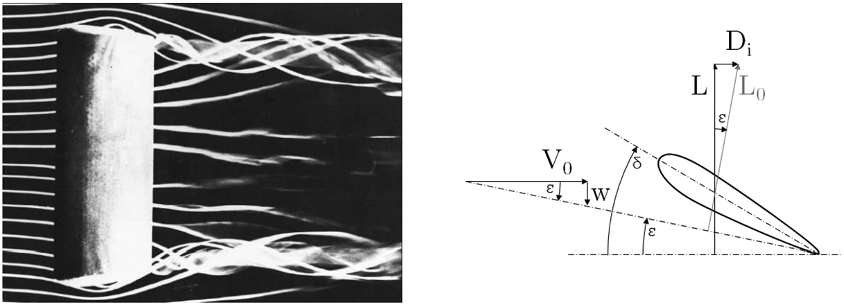
The general effect of the vortex system is to produce a downward velocity component w of the fluid, as in Fig. 4. When this downward flow is combined with the inflow, the local velocity is rotated or inclined to the free stream. This results in a reduction ϵ of the geometric inflow angle δ and the inception of an induced drag ${\mathit{D}}_{\mathit{i}}$ .

Lifting line theory gives the non-dimensional induce drag ${\mathit{C}}_{\mathit{Di}}$ as $$\begin{array}{}\text{(8)}& {\mathit{C}}_{\mathit{Di}}={\displaystyle \frac{{\mathit{C}}_{\mathit{L}}^2}{\mathit{oswalds}·\mathit{\pi }·{\mathit{AR}}_{\mathit{E}}}}.\end{array}$$

The empirical coefficient $\mathit{oswalds}$ represents the induced drag factor, which has a minimum value of $1\mathrm{/}\mathit{\pi }$ . This minimum value was shown by Prandtl [16] using lifting line theory, demonstrating that an elliptical distribution of lift leads to a constant (and minimum) side flow generated by the vortex system. However, this value is likely to be larger and depends on the shape of the surface and on its characteristics such as the taper ratio and sweep of quarter chord. Therefore, the (Oswalds) efficiency factor $\mathit{oswalds}$ is introduced to bring predictions using the drag equation in line with the experimental data.

Fig. 5.

Example of drag components.

The induced drag will add to the parasitic (or section profile) drag ${\mathit{C}}_{\mathit{D}0}$ expressed as $$\begin{array}{}\text{(9)}& {\mathit{C}}_{\mathit{D}0}={\displaystyle \frac{\mathit{formFactor}·2·0.075}{{\mathrm{(}{log}_{10}\mathit{Re}-2\mathrm{)}}^2}}\mathrm{,}\end{array}$$ and the cross flow drag ${\mathit{C}}_{\mathit{D}90}$ (see Fig. 5) expressed as $$\begin{array}{}\text{(10)}& {\mathit{C}}_{\mathit{D}90}=\mathit{cd}90·sin|{\mathit{\delta }}_{\mathit{eff}}{|}^3\mathrm{,}\end{array}$$ in order to give the total drag as $$\begin{array}{}\text{(11)}& {\mathit{C}}_{\mathit{D}}={\mathit{C}}_{\mathit{D}0}+{\mathit{C}}_{\mathit{Di}}+{\mathit{C}}_{\mathit{D}90}.\end{array}$$

The section profile drag ${\mathit{C}}_{\mathit{D}0}$ is expressed as function of the surface Reynolds’ number $\mathit{Re}=\frac{\mathit{meanChord}·{\mathit{V}}_{\mathit{I}}}{\mathit{\nu }}$ (ν is the fluid kinematic viscosity) with the ITTC–1957 model-ship correlation line, including the correction (or form) factor $\mathit{formFactor}$ . A factor 2 is also included since the ITTC–1957 formula uses the wetted surface but for ${\mathit{C}}_{\mathit{D}}$ (see Equation (2)) the lateral projected area is considered: therefore the wetted surface is computed as two times the lateral projected area. The cross flow drag uses also an empirical coefficient, $\mathit{cd}90$ , that is typically 1.2 [7].

3.5. Effective inflow angle

When estimating the lift and drag, it is necessary to use the effective inflow angle ${\mathit{\delta }}_{\mathit{eff}}$ . This may be different from the rudder angle δ relative to ship axes due to the relative position of the rudder and the ship and how the fluid is flowing around the hull and appendages and through a propeller. In fact, when a rudder angle is applied, the ship develops a yaw and drift angle and a yaw and transverse velocity, leading in turn to a cross flow or drift angle at the position of the rudder ${\mathit{\beta }}_{\mathit{R}}=arctan\mathrm{(}\frac{\mathit{v}+{\mathit{x}}_{\mathit{R}}·\mathit{r}}{\mathit{u}}\mathrm{)}$ , as sketched in Fig. 6.

Fig. 6.

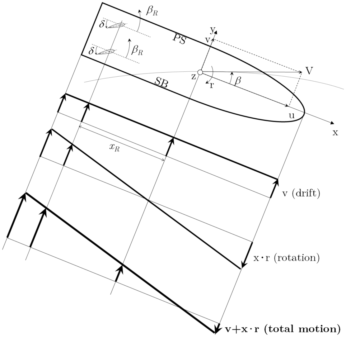
Cross flow when turning and drifting.

The effective inflow angle depends on the effective inflow velocity with respect to the fluid. The effective inflow angle is calculated by estimating a longitudinal and transversal component of the inflow velocity of the rudder with respect to the fluid (in one application point). These components change if a propeller and/or a hull are upstream of the rudder. Simplifying the phenomena, the effects of a propeller and hull (including appendages) upstream of the rudder are basically to straighten the flow, leading to a recovery, or increase, in the effective inflow angle.

In this simplification, the interaction with the propeller is mainly influenced by the propeller thrust loading. The flow passing through the propeller is accelerated and rotated. The swirl and acceleration alter the speed and the inflow angle arriving at the rudder situated aft of the propeller. This influences the forces and moments developed by the rudder. The rudder itself both blocks and diverts the upstream flow onto and through the propeller, which in turn may affect the thrust produced and torque developed by the propeller. The average flow generated by the propeller has axial, transverse, and swirl components. The accelerated (or decelerated) axial component increases (or decreases) the inflow velocity into the rudder. The net effect of the swirl is an effective shift in local inflow angle in one direction above the propeller axis and in the opposite direction below the axis, as sketched in Fig. 7.

Fig. 7.

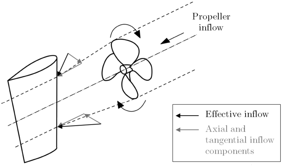
Change of inflow angle due to a propeller upstream.

The direction of the shift depends on the direction of rotation of the propeller. For a rudder with the same area above and below the propeller axis and at zero inflow angle (and neglecting the interaction with the hull and other appendages), the normal forces will cancel, but the drag induced by the lift force on each side of the surface is additional to the section profile drag. With a rudder for which (for instance) the propeller tip protrudes below the tip of the rudder, the effect is an angular offset. Similar effects arise from a variation in lateral separation between propeller and rudder.

Beside the propeller interaction, the hull upstream has also an effect. In particular, two main effects can be seen:

• Due to the presence of the boundary layer, the inflow to the propeller and rudder is reduced with respect to the free stream or ship speed. This effect is taken into account by a Taylor wake fraction. Generally, other components (tangential and swirl) of the propeller velocity are not considered.

• The hull also influences the transversal component of the flow in the ship wake. This deviation of the direction of the fluid flow at the rudder position in comparison with the fluid flow due to drift and yaw movements, is often called flow straightening.

3.5.1. Flow straightening

A flow straightening $\mathit{FWST}$ that is applied on the local cross flow angle (as for instance in [12]) is expressed as $$\begin{array}{}\text{(12)}& {\mathit{\delta }}_{\mathit{eff}}=\mathit{\delta }-\mathit{FWST}·{\mathit{\beta }}_{\mathit{R}}=\mathit{\delta }-\mathit{FWST}·arctan\mathrm{\left(}{\displaystyle \frac{\mathit{v}+{\mathit{x}}_{\mathit{R}}·\mathit{r}}{{\mathit{u}}_{\mathit{I}}}}\mathrm{\right)}\mathrm{,}\end{array}$$ with ${\mathit{u}}_{\mathit{I}}$ the longitudinal component of the rudder inflow (including hull and propeller interaction), v the transversal component of the velocity of the ship with respect to the fluid in a ship-fixed coordinate system, r the yaw rate of the ship with respect to the fluid, ${\mathit{x}}_{\mathit{R}}$ the longitudinal component of the application point of the rudder force w.r.t. a reference point, δ the rudder angle, and ${\mathit{\beta }}_{\mathit{R}}$ the cross flow angle at the rudder position.

Fig. 8.

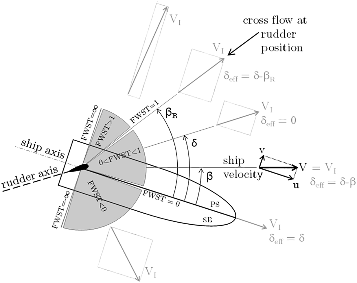
Example of effective inflow angles and corresponding flow straightening factors.

Figure 8 shows the range of possible effective inflow angle ${\mathit{\delta }}_{\mathit{eff}}$ depending on the values of the flow straightening. Figure 8 depicts a turn to starboard, assuming equal, for simplicity sake, the longitudinal component of the velocity of the ship and inflow velocity to the rudder ( ${\mathit{u}}_{\mathit{I}}=\mathit{u}$ ).

Figure 8 shows how, in a turn to starboard, the inflow velocity to the rudder ${\mathit{V}}_{\mathit{I}}$ and consequently the effective inflow angle ${\mathit{\delta }}_{\mathit{eff}}$ change depending on the flow strengthening, so on the interaction with the hull.

• A negative flow straightening means that the flow arrives from starboard, like if it is reattaching from the low pressure side of the hull. This condition might be more conceptual than realistic.

• A flow straightening equal to zero means that the flow is straightened, like if the flow is coming parallel to the rudder chord when at zero degrees.

• A positive flow straightening means that the flow arrives from portside, the same direction that arrives to the hull (high pressure side).

Based on experiments, it is preferred to split the flow straightening in two contributions: one acting on the transversal velocity v and one on the yaw velocity r, leading to an effective inflow angle expressed as $$\begin{array}{}\text{(13)}& {\mathit{\delta }}_{\mathit{eff}}=\mathit{\delta }-arctan\mathrm{\left(}{\displaystyle \frac{{\mathit{v}}_{\mathit{I}}}{{\mathit{u}}_{\mathit{I}}}}\mathrm{\right)}=\mathit{\delta }-arctan\mathrm{\left(}{\displaystyle \frac{\mathit{cdb}·\mathit{v}+\mathit{cdr}·{\mathit{x}}_{\mathit{R}}·\mathit{r}}{{\mathit{u}}_{\mathit{I}}}}\mathrm{\right)}\mathrm{,}\end{array}$$ with ${\mathit{u}}_{\mathit{I}}$ and ${\mathit{v}}_{\mathit{I}}$ respectively the longitudinal and transversal component of the velocity of the rudder with respect to the fluid in a ship-fixed coordinate system.

This allows describing the effect of the transversal and yaw velocities separately, since their effect can vary a lot, matching better towing tank results (as it will be seen for instance in Section 4, where $\mathit{cdb}$ and $\mathit{cdr}$ are different).

In case of multiple rudders, the flow straightening is also differentiated depending whether the rudder is in the inner or outer side of the rotation and drift ( $\mathit{cdb}\text{\_}\mathit{inner}$ , $\mathit{cdb}\text{\_}\mathit{outer}$ , $\mathit{cdr}\text{\_}\mathit{inner}$ , and $\mathit{cdr}\text{\_}\mathit{outer}$ ). In case of a single rudder in the center line of the ship $\mathit{cdb}\text{\_}\mathit{inner}=\mathit{cdb}\text{\_}\mathit{outer}$ and $\mathit{cdr}\text{\_}\mathit{inner}=\mathit{cdr}\text{\_}\mathit{outer}$ .

3.5.2. Velocity

The effective inflow angle is therefore calculated by estimating a longitudinal and transversal component of the velocity of the rudder with respect to the fluid.

Wind tunnel tests carried out for a rudder-propeller only combination, and a rudder “in-behind” condition (a hull with a propeller) are available in the literature (see for instance [14]).

These investigations show that, due to the dominating effects of the propeller, the data for the rudder-propeller only combination can be successfully applied also for the “in-behind” condition when the appropriate hull wake fraction is applied. However, only straight-line flow at high speed and without drift angle was considered in these tests. Results of a rudder-propeller only combination show that the slope of the lift curve remains constant with a changing drift angle. Other tests including a centreboard upstream of the propeller and rudder shows the same.

This confirms the viability of an approach describing the rudder by the velocity and effective inflow angle. However, due to presence of flow separation zones and hull vortices this approach may not be accurate for large drift angles.

The transversal component of the velocity, already introduced in Equation (13) when defining the effective inflow angle, is expressed as $$\begin{array}{}\text{(14)}& {\mathit{v}}_{\mathit{I}}=\mathit{cdb}·\mathit{v}+\mathit{cdr}·{\mathit{x}}_{\mathit{R}}·\mathit{r}.\end{array}$$

The longitudinal component of the velocity of the rudder is mainly influenced by the propeller thrust loading. An approximation to the velocity in the slipstream of the propeller may be made using axial momentum theory while assuming inviscid and incompressible flow. The propeller is assumed to be many bladed, or termed an actuator disc, and capable of imparting axial motion to a fluid, thus producing a thrust on the disc. The velocity in the slipstream of the propeller, or axial-induced velocity ${\mathit{u}}_{\mathit{AI}}$ , is then defined (as in [18]), if the longitudinal component of the velocity of the ship with respect to the fluid in a ship-fixed coordinate system $\mathit{u}⩾0$ as $$\begin{array}{}\text{(15)}& {\mathit{u}}_{\mathit{AI}}=\sqrt{max\mathrm{(}{\mathit{V}}_{\mathit{A}}^2+{\displaystyle \frac{8·\mathit{T}}{\mathit{\rho }·\mathit{\pi }·{\mathit{D}}^2}}\mathrm{,}0\mathrm{)}}-{\mathit{V}}_{\mathit{A}}={\mathit{V}}_{\mathit{A}}·\mathrm{(}\sqrt{1+{\displaystyle \frac{8·{\mathit{k}}_{\mathit{T}}}{\mathit{\pi }·{\mathit{J}}^2}}}-1\mathrm{)}\mathrm{,}\end{array}$$ if $\mathit{u}\mathrm{<}0$ and the thrust of the propeller $\mathit{T}\mathrm{<}0$ as $$\begin{array}{}\text{(16)}& {\mathit{u}}_{\mathit{AI}}=0\mathrm{,}\end{array}$$ and if $\mathit{u}\mathrm{<}0$ and $\mathit{T}⩾0$ as $$\begin{array}{}\text{(17)}& {\mathit{u}}_{\mathit{AI}}=max\mathrm{(}\sqrt{{\displaystyle \frac{8·\mathit{T}}{\mathit{\rho }·\mathit{\pi }·{\mathit{D}}^2}}}+{\mathit{V}}_{\mathit{A}}\mathrm{,}0\mathrm{)}\mathrm{,}\end{array}$$ with ${\mathit{V}}_{\mathit{A}}$ the longitudinal component of the velocity of the propeller with respect to the fluid in a ship-fixed coordinate system defined as $$\begin{array}{}\text{(18)}& {\mathit{V}}_{\mathit{A}}=\mathit{u}·\mathrm{(}1-\mathit{w}\mathrm{)}.\end{array}$$ and w, T, ${\mathit{k}}_{\mathit{T}}$ , J and D respectively Taylor wake fraction, thrust, thrust (open water) coefficient, advance ratio, and diameter of the propeller.

The slipstream contraction as used in the actuator disc theory might not have yet fully developed at the rudder position. For this reason, an empirical correction $\mathit{cad}$ to the axial-induced velocity is made to arrive at an effective velocity. Therefore, the longitudinal component of the velocity of the rudder ${\mathit{u}}_{\mathit{R}}$ (including the axial-induced velocity ${\mathit{u}}_{\mathit{AI}}$ ) results in $$\begin{array}{}\text{(19)}& {\mathit{u}}_{\mathit{R}}=\mathit{u}·\mathrm{(}1-{\mathit{w}}_{\mathit{R}}\mathrm{)}+\mathit{cad}·{\mathit{u}}_{\mathit{AI}}\mathrm{,}\end{array}$$ with ${\mathit{w}}_{\mathit{R}}$ ( $\mathit{wakeFraction}$ ) the rudder wake fraction.

In case of multiple rudders, the wake fraction is also differentiated depending whether the rudder is in the inner or outer side of the rotation and drift ( $\mathit{wakeFraction}\text{\_}\mathit{inner}$ , $\mathit{wakeFraction}\text{\_}\mathit{outer}$ ). In case of a single rudder in the center line of the ship $\mathit{wakeFraction}\text{\_}\mathit{inner}=\mathit{wakeFraction}\text{\_}\mathit{outer}$ .

In addition to a correction for a not fully developed slipstream contraction, there is another aspect to be taken into account, and that is the coverage of the rudder. The propeller slipstream may not cover the rudder completely, since the span is usually larger than the propeller diameter. Therefore, a portion of the surface will be often covered by a slower flow.

MMG [20] proposes to define the longitudinal component of the velocity of the rudder with respect to the fluid in a ship-fixed coordinate system as $$\begin{array}{rl}{\mathit{u}}_{\mathit{I}}=& \mathit{u}·\mathrm{(}1-{\mathit{w}}_{\mathit{R}}\mathrm{)}\\ \text{(20)}& & ·\sqrt{{\displaystyle \frac{{\mathit{D}}_{\mathit{P}}}{{\mathit{H}}_{\mathit{R}}}}·{[1+\mathit{\kappa }·\mathrm{(}\sqrt{1+{\displaystyle \frac{8·{\mathit{K}}_{\mathit{T}}}{\mathit{\pi }·{\mathit{J}}_{\mathit{P}}^2}}}-1\mathrm{\left)}\right]}^2+\mathrm{(}1-{\displaystyle \frac{{\mathit{D}}_{\mathit{P}}}{{\mathit{H}}_{\mathit{R}}}}\mathrm{)}}\mathrm{,}\end{array}$$ where $\frac{{\mathit{D}}_{\mathit{P}}}{{\mathit{H}}_{\mathit{R}}}$ is the ratio between the propeller diameter ${\mathit{D}}_{\mathit{P}}$ and the span of the rudder ${\mathit{H}}_{\mathit{R}}$ . In this way, a weighted average is made between the speed of the rudder with respect to the speed of the fluid inside and outside the propeller disc.

However, this formula will not be correct in the four quadrants. Therefore, it is preferred the weighted average expressed as $$\begin{array}{}\text{(21)}& {\mathit{u}}_{\mathit{I}}=\mathit{\eta }·{\mathit{u}}_{\mathit{R}}+\mathrm{(}1-\mathit{\eta }\mathrm{)}·[\mathit{u}·\mathrm{(}1-{\mathit{w}}_{\mathit{R}}\mathrm{)}]\mathrm{,}\end{array}$$ where η is the portion of rudder span within the propeller disc in the projected y-z plane, as sketched in Fig. 9.

Fig. 9.

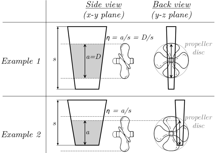
Examples of portion of rudder span within the propeller disc.

3.6. Coordinate systems

Three different coordinate systems can be considered (all with the origin coinciding with the application position of the rudder forces):

1. A coordinate system with an x-axis parallel to the undisturbed inflow fluid stream, a y-axis perpendicular to the inflow, and a z-axis on the rudder rotation axis (positive upwards). In this coordinate system, lift and drag are defined.

2. A coordinate system with an x-axis coinciding with the rudder chord, a y-axis perpendicular to the chord, and a z-axis on the rudder rotation axis (positive upwards). This coordinate system is named rudder-fixed (RF).

3. A ship-fixed (SF) coordinate system, with an x-axis pointing towards the bow, a y-axis towards portside, and a z-axis upwards.

The application position of the rudder forces is usually taken as the longitudinal position of the rudder stock (ship’s aft perpendiculars), the transversal position of the rudder stock, and half of the span as the vertical position. This application position is close to the centre of pressure, even if for rudders with a sweep angle the vertical position may be slightly higher. The choice on the vertical position will affect the ship’s heel angle generated by the rudder.

Assuming a negligible vertical component of the rudder force in a rudder-fixed coordinate system, and the angle in the y-z plane of the stock of the rudder, ${\mathit{\varphi }}_{\mathit{R}}$ , equal to zero for a vertical rudder, the following relations between components in different coordinate systems exist. $$\begin{array}{}\text{(22)}& \mathit{D}=|{\mathit{X}}_{\mathit{RF}}·cos{\mathit{\delta }}_{\mathit{eff}}-{\mathit{Y}}_{\mathit{RF}}·sin{\mathit{\delta }}_{\mathit{eff}}|\text{(23)}& \mathit{L}={\mathit{X}}_{\mathit{RF}}·sin{\mathit{\delta }}_{\mathit{eff}}+{\mathit{Y}}_{\mathit{RF}}·cos{\mathit{\delta }}_{\mathit{eff}}\text{(24)}& {\mathit{X}}_{\mathit{RF}}={\mathit{X}}_{\mathit{SF}}·cos\mathit{\delta }+{\mathit{Y}}_{\mathit{SF}}·sin\mathit{\delta }=-\mathit{D}·cos{\mathit{\delta }}_{\mathit{eff}}+\mathit{L}·sin{\mathit{\delta }}_{\mathit{eff}}\text{(25)}& {\mathit{Y}}_{\mathit{RF}}=-{\mathit{X}}_{\mathit{SF}}·sin\mathit{\delta }+{\mathit{Y}}_{\mathit{SF}}·cos\mathit{\delta }=\mathit{D}·sin{\mathit{\delta }}_{\mathit{eff}}+\mathit{L}·cos{\mathit{\delta }}_{\mathit{eff}}\text{(26)}& {\mathit{X}}_{\mathit{SF}}={\mathit{X}}_{\mathit{RF}}·cos\mathit{\delta }-{\mathit{Y}}_{\mathit{RF}}·sin\mathit{\delta }\text{(27)}& {\mathit{Y}}_{\mathit{SF}}=\mathrm{(}{\mathit{X}}_{\mathit{RF}}·sin\mathit{\delta }+{\mathit{Y}}_{\mathit{RF}}·cos\mathit{\delta }\mathrm{)}·cos{\mathit{\varphi }}_{\mathit{R}}\text{(28)}& {\mathit{Z}}_{\mathit{SF}}=\mathrm{(}{\mathit{X}}_{\mathit{RF}}·sin\mathit{\delta }+{\mathit{Y}}_{\mathit{RF}}·cos\mathit{\delta }\mathrm{)}·sin{\mathit{\varphi }}_{\mathit{R}}\end{array}$$

3.7. Rudder to hull interaction

In a manoeuvre, the total side force will be made up of the contribution from the rudder, but also on the side force developed on the hull due to the rudder to hull interaction. When producing a steering force, the rudder surface will have a high and low pressure side. This will cause also a pressure difference on the hull, leading to an higher total transversal force.

The total transversal force (in a ship-fixed coordinate system) is then calculated as $$\begin{array}{}\text{(29)}& {\mathit{Y}}_{\mathit{total}}={\mathit{Y}}_{\mathit{SF}}·\mathit{chru}.\end{array}$$

The empirical coefficient $\mathit{chru}$ is often expressed as function of the block coefficient [6], because it is assumed to be mainly dependent on the shape of the hull (especially the stern).

However, other characteristics have also an effect on this coefficient. One characteristic is the propeller loading. The higher the loading, the closer $\mathit{chru}$ to 1. This should be taken into account especially when performing manoeuvres at low speed. When performing manoeuvres at speed, the propeller loading is considered to have less influence on $\mathit{chru}$ .

3.8. Four quadrants of operation

The first and second quadrants of operation correspond to a ship sailing forward with respectively positive and negative propeller revolutions. It should be noticed that in the first quadrant the propeller thrust can be positive or negative, depending on the combination of ship’s velocity, propeller revolutions, and propeller’s thrust open water characteristic. The third and fourth quadrants correspond to a ship sailing backward with respectively negative and positive propeller revolutions (also with various combinations of propeller thrust).

A set of wind tunnel tests, which investigated rudder-propeller interaction in four quadrants of operation is reported in [14]. From this investigation, the following observations can be made per quadrant:

1. The results in the first quadrant focused on the part where the ship is sailing forward and the propeller is pushing ahead (positive thrust), therefore this is the first part of the first quadrant, but the main condition ships experience in their operational profile. The rudder has the highest forces here (highest speeds and propeller revolutions), increasing with the propeller loading.

2. In the second quadrant, that corresponds to a ship sailing forward with a propeller pushing astern, the rudder provides low forces and the force slope depends mainly on the propeller thrust.

3. In the third quadrant, that corresponds mainly to a ship sailing backward with a propeller pushing astern, the rudder forces are almost not affected by the propeller. The rudder forces depend on the performance of the lifting surface in open water with an inverse flow.

4. In the fourth quadrant, that corresponds to a ship sailing backward with a propeller pushing ahead, the rudder provides low forces since the flow is quite disturbed and low in speed.

The mathematical model presented here is verified in the four quadrants, considering the following inherent limitations:

1. The model describes the force increase due to the thrust loading in the first quadrant. The model (see Equation (15)) may lack in accuracy when describing the lift decrease in free stream when the thrust is low, due to the extraction of energy from the fluid by the propeller.

2. The model assumes no flow reversal in the second quadrant, so no reverse in lift (see Equation (15)). The more negative the thrust, the smaller the force of the rudder (that might even change sign). Therefore the model might over predict the force, but this is an over prediction of a force that is low in magnitude.

3. The third quadrant is basically an astern free stream condition. The model might under predict the forces due to the (fair) assumption of a negligible interaction with the propeller downstream (see Equation (16)).

4. In the fourth quadrant, the model can describe the axial induced velocity from the propeller. The higher is the thrust, the lower are the rudder forces, but that depends again on the balance between the speed of the ship and the propeller thrust (see Equation (17)).

Fig. 10.

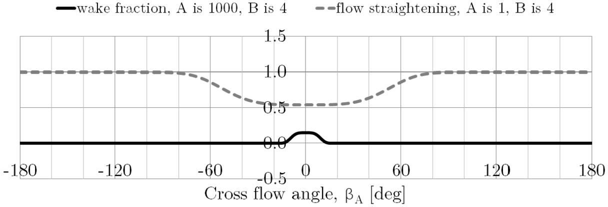
Wake fraction and flow straightening as function of the cross flow angle.

To have a four quadrant model, the following is applied:

• The Taylor wake fraction of the propeller and the rudder are assumed equal to zero when sailing astern. A smooth transition is included from ahead to astern condition, expressed as $$\begin{array}{}\text{(30)}& \mathit{w}=\mathit{w}·{\mathit{e}}^{-\mathit{wakeFractionACoef}·{\mathit{\beta }}_{\mathit{R}}^{\mathit{wakeFractionBcoef}}}.\end{array}$$ Figure 10 depicts this transition as function of the undisturbed cross flow angle ${\mathit{\beta }}_{\mathit{A}}=arctan\mathrm{(}\frac{\mathit{v}+{\mathit{x}}_{\mathit{R}}·\mathit{r}}{\mathit{u}}\mathrm{)}$ . In case of multiple rudders, this applies to the outer rudder.

• The flow straightening coefficients are assumed equal to 1 when sailing astern. A smooth transition is included from ahead to astern condition, expressed as $$\begin{array}{}\text{(31)}& \mathit{cdb}=1-\mathrm{(}1-\mathit{cdb}\mathrm{)}·{\mathit{e}}^{-\mathit{flowStraighteningACoef}·{\mathit{\beta }}_{\mathit{R}}^{\mathit{flowStraighteningBCoef}}}\mathrm{,}\end{array}$$ for instance for $\mathit{cdb}$ (but the same applies for $\mathit{cdr}$ ). Figure 10 shows the transition. In case of multiple rudders, this is valid for the outer rudder.

• The lift slope is decreased when sailing astern. Most rudder surfaces are not symmetrical along the chord and optimized in the lift generation only for inflow angles around zero. The lift slope is then computed as $$\begin{array}{}\text{(32)}& {[{\mathit{dC}}_{\mathit{L}}\mathrm{/}\mathit{d}{\mathit{\delta }}_{\mathit{eff}}]}_{{\mathit{\delta }}_{\mathit{eff}}=0}={[{\mathit{dC}}_{\mathit{L}}\mathrm{/}\mathit{d}{\mathit{\delta }}_{\mathit{eff}}]}_{{\mathit{\delta }}_{\mathit{eff}}=0}·\mathrm{(}1-\mathit{aLR}·{\mathit{e}}^{-\mathit{liftACoef}·{\mathrm{(}|{\mathit{\beta }}_{\mathit{R}}|-\mathit{\pi }\mathrm{)}}^{\mathit{liftBcoef}}}\mathrm{)}\mathrm{,}\end{array}$$ with the empirical coefficient $\mathit{aLR}$ ( $\mathit{asternLiftReduction}$ ) that is 0.3 by default. A smooth transition is included from ahead to astern condition as depicted in Fig. 11.

  

  Fig. 11.

  Lift slope as function of the cross flow angle.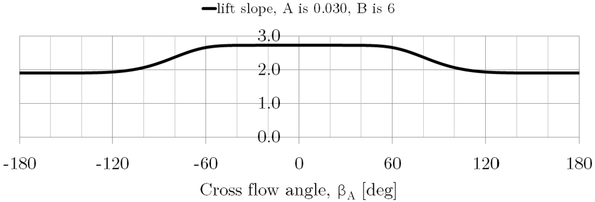

• It is expected that the drag will increase when sailing astern for most rudders. However, a correction to the coefficient $\mathit{formFactor}$ when sailing astern is not implemented.

4. Case study

This section compares the mathematical model with experiments, showcasing the model’s capabilities and shortcomings. Moreover, this section illustrates the procedure to calibrate the empirical coefficients.

A spade rudder behind the KRISO Container Ship (KCS) (see Fig. 12) has been used as a case study to test the model.

Fig. 12.

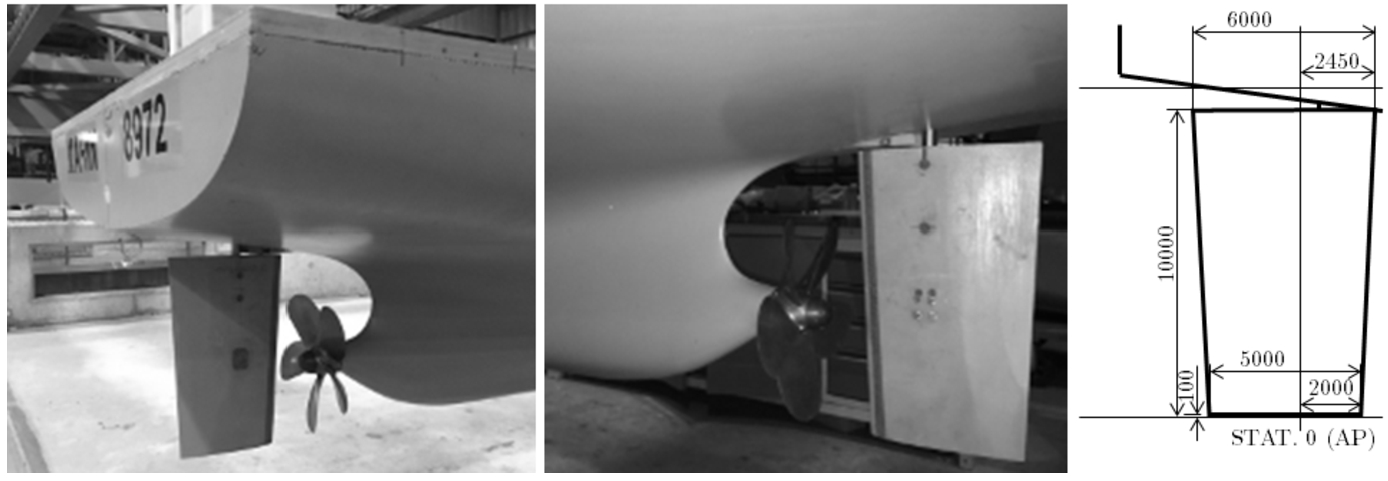
Spade rudder behind the KCS (MARIN model No. 8972).

The KCS is a container ship design that is widely used for manoeuvring simulations and validation.

The main particulars are given in Table 1 in Appendix A.

Several institutes around the world have tested the KCS in free sailing and captive test set-up (even if mostly with a horn rudder instead of a spade rudder).

In January 2019, MARIN conducted a test programme to investigate hydrodynamic loads acting on the KCS (with a spade rudder with and without a propeller upstream) by means of a Computerized Planar Motion Carriage (CPMC) [5] in MARIN’s Seakeeping and Manoeuvring Basin (SMB), at a model scale of 37.89.

The results of these experiments have not been published before.

These experiments include quasi-steady drift angle and yaw rate variations, but also quasi-steady rudder variations.

These experiments provide validation material and are useful to determine the effect on the steering forces of the: rudder angle, ship’s speed, ship’s drift angle, ship’s yaw rate, and propeller induced velocity.

The rudder forces have been measured on the movable part of the rudder with a 2-components frame attached to the rudder (i.e. measuring in a rudder-fixed coordinate system). Therefore the comparison of the forces in a ship-fixed coordinate system should not include the rudder to hull interaction. This means that the empirical coefficient $\mathit{chru}$ has to be subtracted from the mathematical model and this is the reason why a $\mathit{chru}=1$ is used. However, this ship is expected to have a $\mathit{chru}$ of about 1.13.

4.1. Calibration procedure

The following procedure has been applied in order to calibrate the rudder model based on the experiments:

Step 1 (Section 4.2.1). Experiments without propeller are used to estimate (in this order) a rudder wake fraction, a stall coefficient, a form factor and an (Oswalds) efficiency factor. Rudder open water experiments would have been a better first step in order to calibrate the lift slope. Default values have been assumed for the lift slope since rudder open water experiments are not available. The effective aspect ratio is determined based on the rudder and hull geometry.

Step 2 (Section 4.2.2). Experiments with an active propeller but at zero speed are used to estimate the interaction between the propeller and the flow towards the rudder. These experiments are also used to verify the stall behaviour in the presence of a propeller (since stall may change with respect to the case without a propeller). The rudder coverage is determined based on the rudder and propeller geometry and relative position.

Step 3 (Section 4.2.3). Experiments with an active propeller and at speed are used to verify the rudder wake fraction in the presence of a propeller (since the wake field will likely change compared to experiments without a propeller).

Step 4 (Section 4.2.4, 4.2.5, and 4.2.6). Experiments with a drift angle or a yaw rate are used to estimate the flow straightening coefficients.

Step 5 (Section 4.2.7). Experiments with high drift angles and a blocked propeller are used to estimate the corrections for high cross flow angles at the rudder position and four quadrants of operation. A complete validation of the four quadrants of operation would require several experiments with many combinations of rudder angles, ship’s speed, and propeller revolutions. The experiments in this step provide a full range of drift angles, but not the full range of four quadrants of operation. This is discussed further in Section 5.1.

4.2. Validation

The following sections present the experiments, why they are relevant for the validation of the mathematical model, which empirical coefficients are determined, the comparison between experiment and the mathematical model, and the observations from this comparison. The comparison with the models in the literature is done later in Section 5, focusing on the novel features.

The figures present the experimental data with a “dot” marker and the mathematical model with a line. In some cases, experiments of the same type (e.g. rudder angle variations with a drift angle) but multiple conditions (e.g. two drift angles) are depicted in the same figure. The additional conditions are presented with a different colour (“gray”).

Table 1 in Appendix B summarizes the empirical coefficients used in the case study.

4.2.1. Rudder angle variation without propeller

This section compares the mathematical model and the experiments of the rudder behind the hull but without a propeller. These experiments reveal the impact of the upstream hull on the rudder inflow.

Assuming the lift slope is well captured by the typical([4], or Fig. 3 in [12]) default values ( $\mathit{clslope}\text{\_}\mathit{num}$ of 1.95 and $\mathit{clslope}\text{\_}\mathit{denom}$ of 2.25 in Equation (5)), and considering the gap between the rudder top and the stern of the ship (leading the effective aspect ratio to be equal to the geometric aspect ratio, $\mathit{car}=1$ in Equation (3)), Equation (5) becomes: $$\begin{array}{}\text{(33)}& {[{\mathit{dC}}_{\mathit{L}}\mathrm{/}\mathit{d}\mathit{\alpha }]}_{\mathit{\alpha }=0}={\displaystyle \frac{1.95·\mathit{\pi }·1.8}{1.8+2.25}}=\mathrm{2.72.}\end{array}$$

The mathematical model is simplified because there is no interaction with the propeller. This means that $\mathit{eta}$ is 0 ( $\mathit{cad}$ is not used) and Equation (21) becomes: $$\begin{array}{}\text{(34)}& {\mathit{u}}_{\mathit{I}}=\mathit{u}·\mathrm{(}1-{\mathit{w}}_{\mathit{R}}\mathrm{)}.\end{array}$$

Considering a rudder wake fraction ${\mathit{w}}_{\mathit{R}}$ of 0.32 (flow is decelerated by the presence of the hull), a stall coefficient $\mathit{cstall}$ of 3 (stall angle of 30 degrees), a form factor $\mathit{formFactor}$ of 4, and an (Oswalds) efficiency factor $\mathit{oswalds}$ of 0.75, Fig. 13 shows the comparison between the experiment and the mathematical model from a rudder angle variation (±35 degrees) at 12 kn (full scale).

Fig. 13.

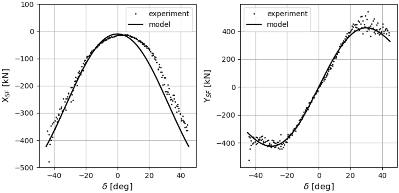
Comparison of a rudder angle variation without a propeller.

The model accurately reproduces the experimental results, however, there exists an unexplained asymmetry in the experiments between positive and negative rudder angles in the longitudinal force which demands further investigation.

4.2.2. Rudder angle variation at bollard pull

This section compares the mathematical model and the experiments of the rudder behind the hull with a propeller, but at bollard pull (i.e. active propeller pushing ahead but ship’s speed at 0 kn). These experiments provide insight into the interaction between the propeller and the flow towards the rudder.

With the ship stationary in the water, Equation (21) becomes: $$\begin{array}{}\text{(35)}& {\mathit{u}}_{\mathit{I}}=\mathit{cad}·\sqrt{{\displaystyle \frac{8·\mathit{T}}{\mathit{\rho }·\mathit{\pi }·{\mathit{D}}^2}}}.\end{array}$$

Therefore the empirical correction $\mathit{cad}$ to the axial-induced velocity can be determined. With a $\mathit{cad}$ of 0.55, Fig. 14 shows the comparison between the experiment and the mathematical model for a rudder angle variation (±35 degrees) at 0 kn, with a propeller pushing ahead with different propeller revolutions, so propeller loadings (73.5, in black in Fig. 14, and 149 rpm, in gray).

Fig. 14.

Comparison of a rudder angle variation at bollard pull (2 propeller revolutions: 73.5 rpm in black and 149 rpm in gray).

The presence of the propeller complicates the flow leading to a different stall behaviour. If without the propeller the soft stall has a peak at about 30 degrees (see Fig. 13), with a propeller the stall is delayed to about 52.5 degrees (in fact $\mathit{cstall}$ is 1.42 in this case). Having the coefficient $\mathit{cstall}$ allows to correct for this effect, but not for the difference between positive and negative rudder angles. This difference can be explained for a large part by the direction of rotation of the propeller.

4.2.3. Rudder angle variation at speed

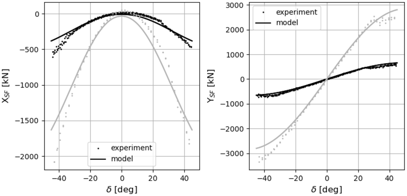
This section compares the mathematical model and the experiments of the rudder behind the hull with a propeller, but this time at speed (the ship has a speed of 12 kn). These experiments provide insight into the rudder wake fraction.

Although the rudder wake fraction was already found without the propeller, it may vary with the propeller upstream.

With a wake fraction of 0.15 (instead of 0.32 in the case without the propeller), Fig. 15 shows the comparison between the experiment and the mathematical model from a rudder angle variation (±35 degrees) at 12 kn, with a propeller pushing ahead with different propeller revolutions, so propeller loadings (73.5, in black in Fig. 15, and 149 rpm, in gray).

Fig. 15.

Comparison of a rudder angle variation at speed (2 propeller revolutions: 73.5 rpm in black and 149 rpm in gray).

The 73.5 rpm correspond to the propeller revolutions required to sail ahead at 12 kn. The 149 rpm pertain to an overload condition. An overload condition is typical for instance in the steady part of a turning circle.

The corrected wake fraction (with respect to the experiment without propeller) and the empirical correction $\mathit{cad}$ for the axial-induced velocity as estimated in the bollard pull experiment (see Section 4.2.2) can predict well the increase in the rudder forces due to the ship’s speed. The experimental results are accurately reproduced by the model, especially for the transversal force. However, differences exist at high rudder angles, where the soft stall occurs: the model over predicts the transversal force in the experiment with 73.5 rpm and under predicts the transversal force in the experiment with 149 rpm.

4.2.4. Rudder angle variation with a drift angle

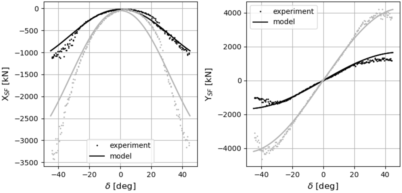
This section compares the mathematical model and the experiments of the rudder behind the hull with a propeller, at speed (the ship has a speed of 18 kn), but also with a drift angle (coinciding with the undisturbed cross flow angle ${\mathit{\beta }}_{\mathit{A}}$ ) of −8 and 20 degrees. These experiments provide insight into the flow straightening coefficient, looking in particular at the contribution due to the transversal speed (drift angle).

The experiments is carried out with a fixed drift angle (no yaw rate), therefore Equation (13) becomes: $$\begin{array}{}\text{(36)}& {\mathit{\delta }}_{\mathit{eff}}=\mathit{\delta }-\mathit{\alpha }=\mathit{\delta }-arctan\mathrm{\left(}{\displaystyle \frac{{\mathit{v}}_{\mathit{I}}}{{\mathit{u}}_{\mathit{I}}}}\mathrm{\right)}=\mathit{\delta }-arctan\mathrm{\left(}{\displaystyle \frac{\mathit{cdb}·\mathit{v}}{{\mathit{u}}_{\mathit{I}}}}\mathrm{\right)}.\end{array}$$

With a flow strengthening $\mathit{cdb}$ factor of 0.54, Fig. 16 shows the comparison between the experiment and the mathematical model from a rudder angle variation (±35 degrees) at 18 kn, with a propeller pushing ahead with 108 rpm, and with two drift angles (in one experiment −8 degrees, in black in Fig. 16, and in the other 20 degrees, in gray).

Fig. 16.

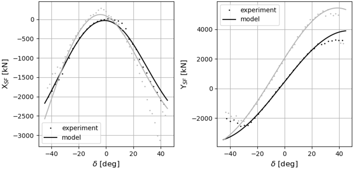
Comparison of a rudder angle variation with two drift angles (−8, in black, and 20 degrees, in gray).

The experimental results are accurately reproduced by the model, showing the shift in the force due to the drift angle. It should also be noticed that these results (especially at 20 degrees) make use of the correction of the flow straightening coefficients and wake fraction as function of the undisturbed cross flow angle as in Fig. 10. However, differences exist at high rudder angles, where the soft stall occurs. The longitudinal force in the case of 20 degrees of drift angle and negative rudder angles is also different.

4.2.5. Rudder angle variation with a yaw rate

This section compares the mathematical model and the experiments of the rudder behind the hull with a propeller, at speed (the ship has a speed of 18 kn), but also with a yaw rates (non-dimensional yaw rate $\mathit{\gamma }=\mathit{r}·{\mathit{L}}_{\mathit{PP}}\mathrm{/}\mathit{V}$ of 0.2 and 0.8, with $\mathit{V}=\sqrt{{\mathit{u}}^2+{\mathit{v}}^2}$ ). These experiments provide insight into the flow straightening coefficient, looking in particular at the contribution due to the yaw rate.

The experiments is carried out with a fixed yaw rate (no drift angle), therefore Equation (13) becomes: $$\begin{array}{}\text{(37)}& {\mathit{\delta }}_{\mathit{eff}}=\mathit{\delta }-\mathit{\alpha }=\mathit{\delta }-arctan\mathrm{\left(}{\displaystyle \frac{{\mathit{v}}_{\mathit{I}}}{{\mathit{u}}_{\mathit{I}}}}\mathrm{\right)}=\mathit{\delta }-arctan\mathrm{\left(}{\displaystyle \frac{\mathit{cdr}·{\mathit{x}}_{\mathit{R}}·\mathit{r}}{{\mathit{u}}_{\mathit{I}}}}\mathrm{\right)}.\end{array}$$

With a flow strengthening $\mathit{cdr}$ factor of 0.71, Fig. 17 shows the comparison between the experiment and the mathematical model from a rudder angle variation (±35 degrees) at 18 kn, with a propeller pushing ahead with 108 rpm, and with two yaw rates (in one experiment $\mathit{\gamma }=0.2$ , in black in Fig. 17, and in the other $\mathit{\gamma }=0.8$ , in gray). The non-dimensional yaw rates of 0.2 and 0.8 correspond to an undisturbed cross flow angle ${\mathit{\beta }}_{\mathit{A}}$ of $-5.7$ and $-21.8$ degrees.

Fig. 17.

Comparison of a rudder angle variation with two yaw rates (γ of 0.2, in black, and 0.8, in gray).

The experimental results are accurately reproduced by the model, showing the shift in the force due to the yaw rate. However, differences exist at high rudder angles, where the soft stall occurs.

It is also interesting to notice that the flow straightening coefficient due to a yaw rate ( $\mathit{cdr}=0.71$ ) is different from the one due to a drift angle ( $\mathit{cdb}=0.54$ , see Section 4.2.4). As anticipated in Section 3.5.1, this explains why different factors should be considered.

4.2.6. Drift angle and yaw rate variation

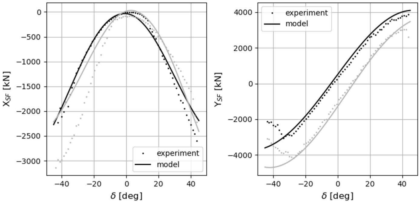
In addition to rudder angle angle variations, drift angle and yaw rate variations are available. This section compares the mathematical model and the experiments of the rudder behind the hull with a propeller, at speed (the ship has a speed of 18 kn), with a fixed rudder angle of 20 degrees during a yaw rate or drift angle (−20 to 20 degrees) variation. These experiments provide insight into the flow straightening coefficient.

With the flow straightening coefficients already determined (see Section 4.2.4 and 4.2.5), Fig. 18 shows the comparison between the experiment and the mathematical model (this time focusing on the transversal force) from a yaw rate variation (±0.8 or ${\mathit{\beta }}_{\mathit{A}}\pm 22$ degrees, on the left) and a drift angle variation (±20 degrees, on the right) at 18 kn, with a propeller pushing ahead with 108 rpm.

Fig. 18.

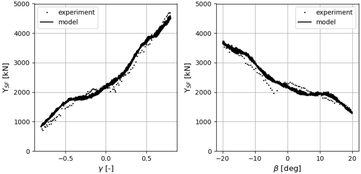
Comparison of a yaw rate (left) and drift angle (right) variation with a fixed rudder angle of 20 degrees.

The experimental results are accurately reproduced by the model, showing the shift in the force due to the ship’s yaw rate and drift angle.

It should also be noticed that these results make use of the correction of the flow straightening coefficients and wake fraction as function of the undisturbed cross flow angle as in Fig. 10 and Fig. 11.

As anticipated in Section 3.5.1 and already remarked in Section 4.2.5, even though the two variations are similar in terms of undisturbed cross flow angle ${\mathit{\beta }}_{\mathit{A}}$ , the forces are quite different. This explains again why different flow straightening coefficients should be considered. It would not be possible to predict correctly both situations with a flow straightening factor as in Equation (12), considering only the cross flow angle at the rudder and without separating the effect due to a drift angle from the one due to a yaw rate.

4.2.7. Drift angle variation, ahead and astern velocity

This section extends the drift angle variation in Section 4.2.6. This section compares the mathematical model and the experiment of the rudder behind the hull, at speed, with a fixed rudder angle of 0 degrees during a drift angle variation, but now including also a negative speed, so reaching a drift angle greater than 90 degrees, and with a blocked propeller. These experiments provide insight into the flow straightening coefficient at high drift angles.

With the flow straightening coefficients already determined in Section 4.2.4, Fig. 19 shows the comparison between the experiment and the mathematical model (focusing on the transversal force) from a drift angle variation (from −30 degrees up to 210 degrees) at 12 kn, with a blocked propeller (0 rpm).

Fig. 19.

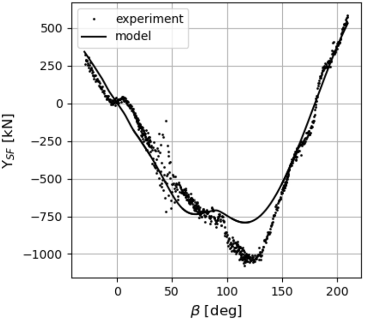
Comparison of a drift angle variation with a fixed rudder angle of 0 degrees and a blocked propeller.

The experimental results are realistically reproduced by the model, showing a good prediction when sailing astern (around 180 degrees): the good prediction around 180 degrees justifies the modelling choice of a lift slope correction when sailing astern, as described in Fig. 11.

However, some discrepancies can be seen:

• Around 0 degrees; this difference is larger than in Fig. 18 because of the effects of a blocked propeller. However the magnitude is also much lower (at −30 degrees, the force is about 250 kN with a blocked propeller and 3500 kN with an active propeller).

• Around 120 degrees; here the experiment presents a peak that is only partially captured by the model.

5. Overview of novel features

The limitations of the models available in the literature have been highlighted in Section 1. Novel features of the rudder mathematical model presented in this paper have been introduced in Section 3 and partially validated in Section 4. These features include in particular the extension of the mathematical model to:

• Describe suitably the interaction with the propeller in four quadrants of operation. This is done by a proper model of the axial-induced velocity.

• Include the effects of a lateral or vertical misalignment between the rudder and the propeller upstream in the rudder coverage.

• Ensure realistic behaviour at high drift angles at the position of the rudder. This is done by including the cross flow drag and by correcting the flow straightening, the wake fraction, and the lift slope as function of the drift angle at the position of the rudder.

• Correct properly for the stall angle.

• Allow more flexibility, by defining additional empirical coefficients.

In the next sections, these extensions are further discussed and compared to the MMG rudder model [20], previous publications [8,9] of MARIN rudder models, and other models in the literature, such as [3].

5.1. Four quadrants of operation

As shown in Fig. 19 in Section 4.2.7, the present model can realistically predict the rudder force with a blocked propeller. A blocked propeller (no propeller revolutions) with a ship sailing forward and backward defines two points in the four quadrants of operation, in particular the conditions when the hydrodynamic pitch angle of the propeller ${\mathit{\beta }}^{\mathrm{\star }}$ [13] is ±90 degrees. The models from the literature in [10,12,15,20], and [11] lead to a mathematical singularity since the propeller revolutions n equals zero and therefore in $\mathit{J}=\frac{{\mathit{V}}_{\mathit{A}}}{\mathit{n}·{\mathit{D}}_{\mathit{P}}}$ there is a division by zero. The models in [8] will also encounter a problem because it will require to compute the square root of a negative number since ${\mathit{V}}_{\mathit{A}}^2+\frac{8·\mathit{T}}{\mathit{\pi }·\mathit{\rho }·{\mathit{D}}^2}$ is negative (see Equation 7.16 in [8]). Therefore a comparison with these models is not even possible in this case.

Even though a full validation is not presented in this paper (no experiments were conducted for instance with a rudder angle and a propeller pushing astern for the ship sailing forward and backward), the mathematical model presented here shows already an improvement with respect to the models from the literature.

As described in Section 3.8, the model presented in this paper is verified against wind tunnel tests, which investigated rudder-propeller interaction in four quadrants of operation, as reported in [14].

A similar verification is presented for the case study (KCS with a spade rudder with a propeller upstream, see Section 4) in Fig. 20.

Fig. 20.

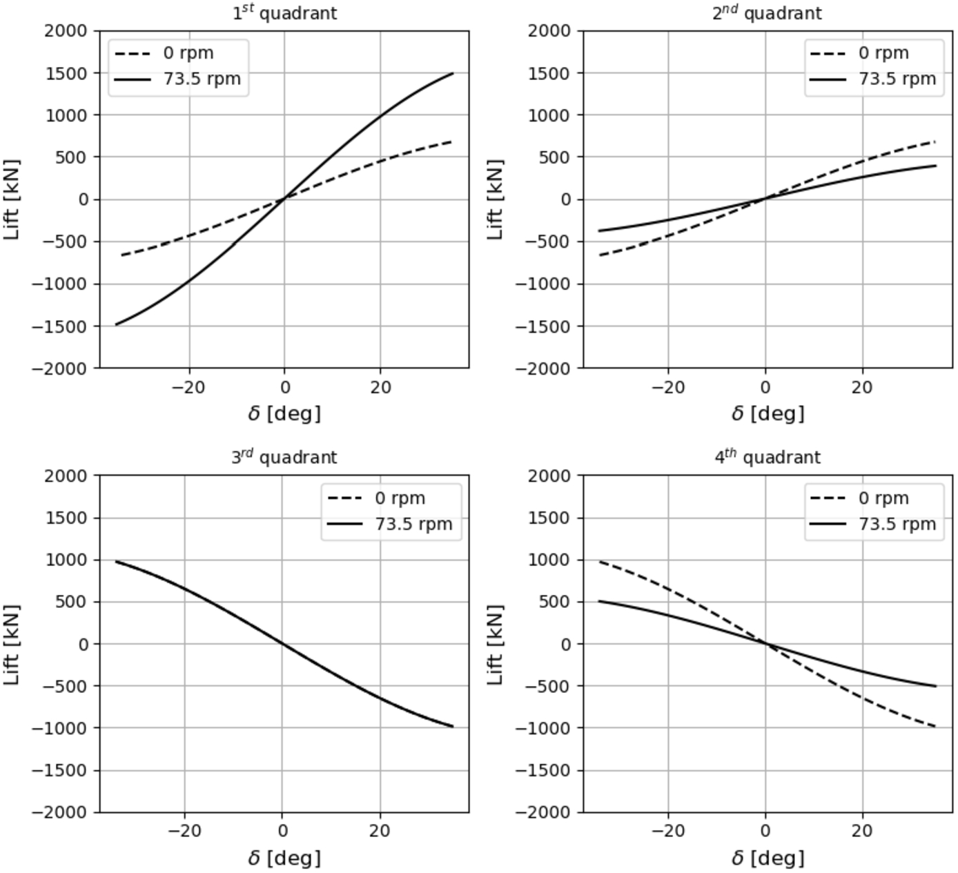
Verification of the four quadrants of operation for the case study.

The results in the first quadrant in Fig. 20 show the increase in lift with the propeller loading. The results in the second quadrant show the decrease in lift with respect to the first quadrant, and the additional decrease due to the interaction with the propeller. The results in the third quadrant, basically an astern free stream condition, show how the rudder is not affected by the propeller (assuming a negligible interaction with the propeller downstream). The lift is lower (even if the wake fraction is zero) because the lift slope decreases when sailing astern. The results in the fourth quadrant show how the lift decreases due to the propeller (the higher the thrust, the lower the lift).

The modification in the model presented here extends therefore the applicability of the model.

5.2. Rudder coverage

In addition to the verification described in Section 5.1, showing for the case study how practically Equation (21) works, it should also be mentioned that the rudder coverage is treated differently from the literature.

While the literature [11,20] uses the ratio between propeller diameter and rudder span, the mathematical model presented here considers the propeller disc (see Fig. 9).

In case of a rudder not aligned with the propeller transversal or vertical position, the rudder coverage from the literature can be overestimated, leading to an inaccurate estimation of the inflow velocity. In fact, if the rudder is less in the accelerated flow coming from the propeller, the force should reduce (even though the ratio between propeller diameter and rudder span is the same).

The modification in the model presented here extends therefore the applicability of the model.

5.3. High drift angles at the position of the rudder

In order to compare qualitatively the model presented here with the literature, where there are no corrections for high drift angles, Fig. 21 shows how a model without corrections for the case study would compare.

Fig. 21.

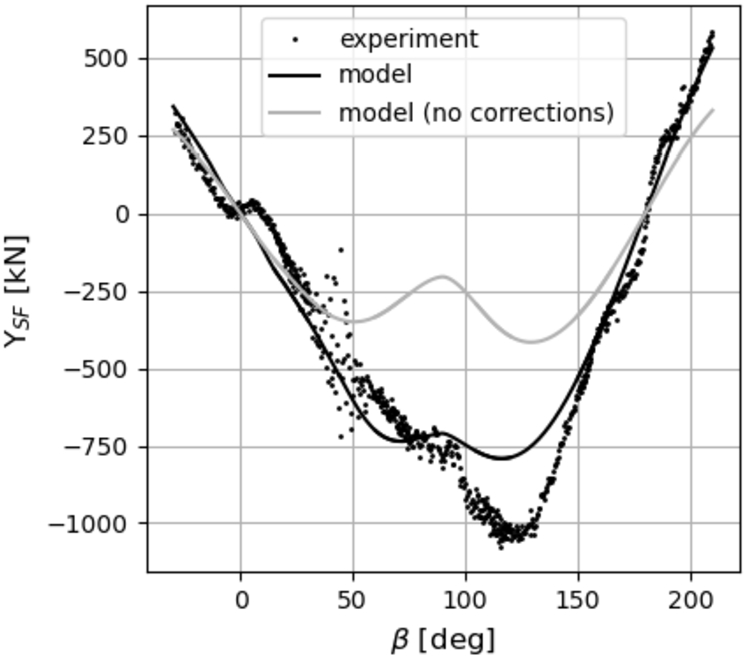
Comparison of a drift angle variation with a fixed rudder angle of 0 degrees and a blocked propeller, with and without four quadrants corrections.

The corrections described in Section 3.8 include a description of the wake fraction, flow straightening coefficients, and lift slope as function of the undisturbed cross flow angle (see Fig. 10 and Fig. 11).

The comparison in Fig. 21 shows how constant coefficients would not be able to describe the rudder force in the whole range: in fact even if the slope is acceptable around zero degrees, as soon as the drift angle increases the model starts to deviate; when looking at the results around 180 degrees (astern sailing), it is also clear that a different lift slope is needed.

For this reason, the mathematical model presented here shows an improvement with respect to the literature.

5.4. Stall angle

Most of the models in the literature uses a function with the sine and cosine of the rudder angle to describe the rudder force. This means that the stall angle is assumed to be always at 45 degrees.

Table 5.2 and 5.5 in [14] tabulates the stall angles from free-stream data (so without a propeller upstream) of respectively the nine model foils from [19] and the control surfaces with different section types (from flat plates, to typical NACA profiles, up to Institute für Schiffbau, Ifs, sections) from [17]. The tables show that the stall angle can vary greatly, with values from 13.5 up to 48 degrees.

Therefore, a rudder mathematical model should be able to define the correct stall angle, as it happens for the rudder mathematical model described here (see Section 3.3).

For this reason, the mathematical model presented here shows an improvement with respect to the literature.

5.5. Flexibility

The results in Table 5.2 and 5.5 in [14] shows also how the lift slope and the drag can vary. Therefore to make the rudder model more flexible to describe different rudders (also in type, as fishtail rudders), additional empirical coefficients and extensions to the formula are introduced especially to:

• Correct the lift slope; this can be done directly with the coefficient $\mathit{clslope}\text{\_}\mathit{num}$ or $\mathit{clslope}\text{\_}\mathit{denom}$ in Equation (5), or indirectly when changing the coefficient $\mathit{car}$ in Equation (3) defining the effective aspect ratio (for instance if the rudder has an end plate). Default values based on theoretical and empirical background (see [4], or Fig. 3 in [12]) are often used in the literature, but these might be only valid for standard spade rudders. The same applies to the effective aspect ratio that is often considered the same as the geometric one ( $\mathit{car}=1$ ), even if this might often be the case. In fact, as described in Fig. 5.101 and 5.104 in [14], the rudder root gap and the hull shape on top of the rudder can decrease $\mathit{car}$ up to 1, especially with an increasing rudder angle.

• Correct the drag; this can be done by correcting the parasitic drag with the coefficient $\mathit{formFactor}$ (see Equation (9)), the lift induced drag with the coefficient $\mathit{oswalds}$ (see Equation (8)) and the cross flow drag with the coefficients $\mathit{cd}90$ (see Equation (10)). This is also possible because of the extension of the drag formulation with respect to the literature, considering usually only the lift induced drag (so one of the three components in the model presented here).

The modifications in the model presented here extend therefore the applicability of the model.

6. Conclusions

This paper offers a comprehensive insight into the mathematical model utilized in MARIN’s time domain software to represent the hydrodynamic loads excited by a rudder. With a detailed theoretical explanation, the paper demonstrates how the model has been designed to provide a robust and reliable representation of rudder forces.

Furthermore, the model of a spade rudder behind the KCS container ship with and without a propeller upstream has been tested against experiments to illustrate how the model performs in practice. The validation shows that the model accurately reproduces the experimental results, however there are some discrepancies especially around stall angle and for the longitudinal force in some of the considered cases.

This rudder mathematical model is expected to be more widely applicable than its predecessors. This is guaranteed by novel features and by the presence of additional empirical coefficients to allow flexibility.

The novel features of the mathematical model presented here allow to describe:

• Scenarios in the four quadrants of operation, therefore with combinations of positive or negative ship’s speed and positive or negative propeller revolutions.

• Designs with rudders not aligned with the propellers, therefore only partially covered by the propeller outflow.

• Situations with all kinds of inflow to the rudder, including situations with a cross flow, like when drifting in beam waves or when turning on the spot.

• Operations with rudder angles above the typical maximum angle of 35 degrees, like for instance when dealing with inland ships.

Even though not all the novel features could be validated, the authors have explained why different choices in the modelling are needed.

Despite the inherent assumptions of a reduced-order mathematical model, the authors would like to emphasize that the present rudder mathematical model, as most of the models in the literature, does not describe:

• The net effect of the swirl (or tangential) component of the propeller velocity. Therefore, the shift in local rudder inflow angle due to this effect is neglected. The reason is that a robust and simple formula to describe this effect was not found.

• The added inertia of the rudder, so the hydrodynamic loads in phase with the acceleration. This component is often neglected, being of lower magnitude with respect to the hull, or included in other sub-models, such as the hull mathematical model (but often considering the rudder at a fixed angle of zero degrees).

Additional investigations on these aspects and further validation are intended. The further validation should include the comparison to experiments with more combinations of speeds and propeller thrusts, the validation for ships with multiple rudders, and the analysis of the yaw, heel and torque moment caused by the rudder.

Furthermore, it is important to address default values for the empirical coefficients to make it easier to use this model when experimental data is not available.