
Abstract
The article presents a random neural Q-learning strategy for the obstacle avoidance problem of an autonomous mobile robot in unknown environments. In the proposed strategy, two independent modules, namely, avoidance without considering the target and goal-seeking without considering obstacles, are first trained using the proposed random neural Q-learning algorithm to obtain their best control policies. Then, the two trained modules are combined based on a switching function to realize the obstacle avoidance in unknown environments. For the proposed random neural Q-learning algorithm, a single-hidden layer feedforward network is used to approximate the Q-function to estimate the Q-value. The parameters of the single-hidden layer feedforward network are modified using the recently proposed neural algorithm named the online sequential version of extreme learning machine, where the parameters of the hidden nodes are assigned randomly and the sample data can come one by one. However, different from the original online sequential version of extreme learning machine algorithm, the initial output weights are estimated subjected to quadratic inequality constraint to improve the convergence speed. Finally, the simulation results demonstrate that the proposed random neural Q-learning strategy can successfully solve the obstacle avoidance problem. Also, the higher learning efficiency and better generalization ability are achieved by the proposed random neural Q-learning algorithm compared with the Q-learning based on the back-propagation method.
Keywords
Introduction
Obstacle avoidance is one of the primary tasks for autonomous mobile robots (AMRs), whose purpose is to enable mobile robots to arrive at the target points without colliding with any obstacles in the working environment. A lot of approaches have been developed to solve this problem, such as grid methods,1–3 potential field methods,4,5 fuzzy logic methods,6,7 and so on. These methods are usually based on specific environment models and rely on more priori knowledge, such as experience and rules. Also they lack self-learning abilities to adapt to various unknown environments. Once there is a change in the environment or task, the corresponding strategies need to be updated manually. Thus, it is better to incorporate self-learning function to realize autonomous obstacle avoidance (AOA) in the unknown environments. Reinforcement learning (RL) is considered to be a more appropriate method to accomplish the task by directly interacting with environment without requiring any prior knowledge about the environment models. RL is a learning process based on a set of mapping from states of environment to actions through maximizing a value function that estimates the expected cumulative reward in the long term. The most well-known method is Q-learning, in which the value function is the function of state–action pairs, called Q-value. However, ordinary Q-learning can only deal with discrete states and actions. In the AOA task, states of environment are generally continuous and Q-learning cannot directly used for it.
To handle this problem, many research studies8–13 have extended the Q-learning method to deal with continuous situation spaces by means of neural networks. In all these works, different neural networks including feedforward and recurrent networks are used to approximate the Q-values pertaining to specific situations with its universal approximation capability. Also the parameters of the networks are updated based on the back-propagation (BP) learning algorithm where gradients are computed by propagation from the output to the input. As we know, there are several practical issues that BP learning algorithms suffer from. Specifically, the BP learning method easily converges to a local minimum if the estimated Q-value is not convex with respect to its parameters. 14 It is undesirable that the learning algorithm stops at a local minimum if it is located far above a global minimum. Meanwhile, the BP learning algorithm has a very slow convergence speed in most applications, including Q-learning. This will take the robot too long and too many collisions to arrive at the goal.
Recently, a new fast neural learning algorithm referred to as extreme learning machine (ELM) has been developed for single-hidden layer feedforward networks (SLFNs) in Huang et al., 15 Huang and Siew, 16 and Huang et al.17,18 ELM and its different improvements19–21 have been successfully applied in some applications.22–30 It has been shown that ELM can provide better generalization performance at extremely high learning speed.17,18,27,28,30 The universal approximation capability of ELM has been rigorously proved 31 using an incremental method (named incremental extreme learning machine (I-ELM)). An online sequential learning version of the batch ELM (OS-ELM) has been developed. 32 In OS-ELM, the parameters of hidden nodes in the SLFNs are randomly generated and fixed. Based on this, the output weights are analytically determined. OS-ELM can learn the training data not only one-by-one, but also chunk by chunk (with fixed or varying length) and discard the data for which the training has already been done.
In this article, a novel random neural Q-learning (RNQL) approach is proposed for collision-free behavior selection of an AMR in unknown environments. In the strategy, the SLFN is used as the function approximator to estimate the Q-value. Different from the existing methods, the parameters of the SLFN are adjusted based on OS-ELM. Furthermore, to achieve a fast convergence speed, the initial output weights in the initialization phase of OS-ELM are estimated subjected to quadratic inequality constraint. Simulation results show that this proposed method not only obtains high learning efficiency, but also produces good generalization performance compared with the existing Q-learning algorithms updated based on the BP technology.
This article is organized as follows. In section “Problem definition,” the problem definition for the AOA of an AMR is presented. The details of the proposed RNQL method are described in section “RNQL algorithm.” Section “Performance evaluation” presents a quantitative performance comparison between RNQL algorithm with back-propagation Q-learning (BPQL) algorithm for the obstacle avoidance problem of an AMR. Section “Conclusion” summarizes the conclusions from this study.
Problem definition
The study presented in this article is applicable to any AMR, independent of its size and type. Here, we discuss our study with a special reference to an AMR consisting of one unactuated and not-sensed steer wheel and two actuated and sensed wheels. The detailed configuration of the robot is shown in Figure 1. This type of chassis provides three degrees of freedom (3-DOF) locomotion in a vehicle coordinate denoted by

Sketch of the AMR.

Configuration of sensors.
When the environments are unknown, the obstacle avoidance problem of an AMR can be considered as a behavior selection task. In this task, the robot can automatically produce a correct action of reaching the destination without collision according to the environment information perceived by the sensors equipped on the robot. The task details are shown in Figure 3. The blue dots represent the trace of the robot and the red circle dot is the goal represented by
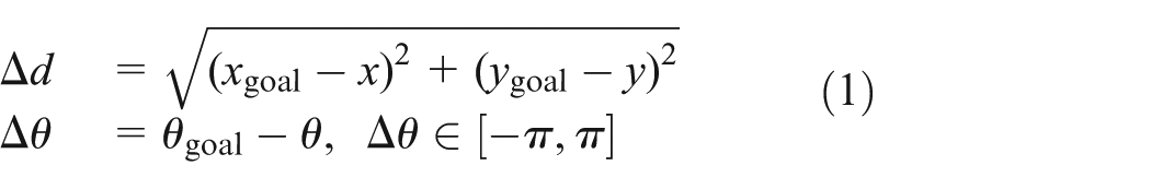

Diagram of control variables.
In order to navigate the mobile robot to its goal, it is assumed that these variables are always known at each time step t. Therefore, an obstacle avoidance task is to obtain these variables,

Structure of RL.
But Q-learning is usually applied to the discrete set of states and the Q-values of state–action pairs are stored in a table. As the perceived states of an AMR are continuous, a large storage space is required to store all the possible state–action pairs. In order to solve these problems, the SLFN is applied to approximate the Q-function and used as a Q-value estimator. The state of the robot is the inputs of the neural network and the outputs are the Q-values of all the actions. It is worth noting that the AMR in our work is operating in changing and unknown environments and it needs to explore its environment from consecutively collecting sufficient samples of the necessary experience for learning. Thus, a RNQL method with the online learning capability is employed so that the AMR can adapt to the environment without human intervention. In the proposed method, the SLFN is used to approximate the Q-value, and the parameters of hidden nodes in the SLFN are assigned randomly based on the OS-ELM algorithm. The output weights are recursively updated analytically. The design details are described below.
RNQL algorithm
In this section, the design process of the proposed RNQL is presented. The mathematical models of the SLFN and the ELM used in the design are first reviewed.
Mathematical description of unified SLFN
The output of a SLFN with

where

where
For RBF hidden nodes with the Gaussian or triangular activation function,

where
ELM algorithm
For N arbitrary distinct samples

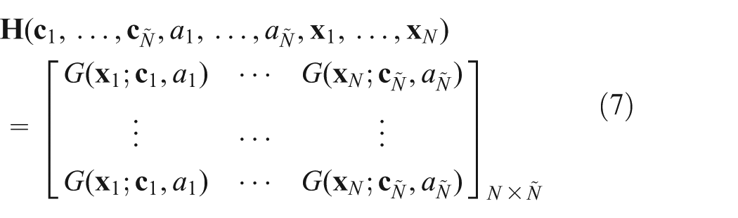
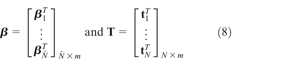
Equation (5) can be written compactly as follows

where
It has been proven that a SLFN with the ELM algorithm can approximate any a nonlinear continuous function to an arbitrary accuracy. 18 The following lemma is introduced.
Lemma 1
For a SLFN with additive or RBF hidden nodes and activation function
The ELM algorithm offers a fast neural learning algorithm. All the parameters of the hidden nodes
RNQL algorithm
In the study, the obstacle avoidance task can be achieved by two behaviors: avoidance and goal-seeking. The former behavior is inherently nearsighted as it only considers how to avoid obstacles and ignores whether it causes the vehicle to deviate from the goal, whereas the latter behavior is inherently farsighted as it enables the vehicle to move toward the goal disregarding potential collisions. Thus, the two behavior modules are independent of each other and their functions always conflict. To achieve their respective goals, they are independently designed by the proposed RNQL algorithm. But the state space from the two modules is different, although the learning process is similar. For the obstacle avoidance module, the element of the state
The two behaviors are independently designed and then are combined to navigate the robot in a new environment without further learning when their mapping between input state space and output action space is correctly established. To efficiently combine the two behaviors, a switching function is used as the behavior selector to choose one behavior to be used at next action step, which is defined as follows

where r represents the avoidance region and i is any one of the set
Estimation of Q-value
In our proposed RNQL algorithm, a SLFN is used to estimate the Q-value, which is given as follows

where
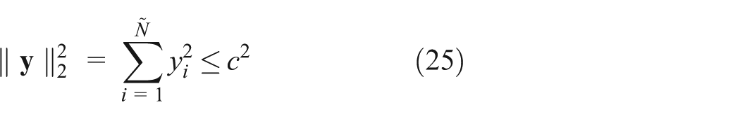
OS-ELM consists of two phases, namely an initialization phase and a sequential learning phase. In the initialization phase, the initial output weights
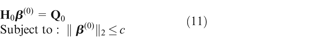
where c is a constant value and

The problem to the solution

The singular value decomposition could be used to solve equation (13). The details are presented in section “Least-square minimization with a quadratic inequality constraint.”
On each step of interaction, the Q-value function is updated with the following equation
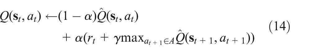
where

Based on equation (14), the output weights

where

After a period of learning, the value of

The optimal policy (equation (18)) is used to choose the best action. According to the state–action value
However, at the whole learning phase of the proposed algorithm, in order to explore all possible actions, the Boltzmann probability distribution is employed here to select a possible action

where

where
Least-square minimization with a quadratic inequality constraint
In this section, the singular value decomposition
35
will be used to solve equation (13), where

where

and then problem (13) transforms to

where

and the constraint equation
facilitate the analysis of the least-square minimization with a quadratic inequality constraint problem.
Consideration of equation (24), the vector

is a minimizer of

to equation (13). If this is not the solution of minimum two norms, we assume that
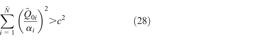
This implies that the solution to the least-square minimization with a quadratic inequality constraint problem occurs on the boundary of the feasible set. Thus, our remaining goal is to

To solve this problem, Lagrange multipliers method is popular. Defining

we see that the equations

Assuming that the matrix of coefficients is nonsingular, this has a solution
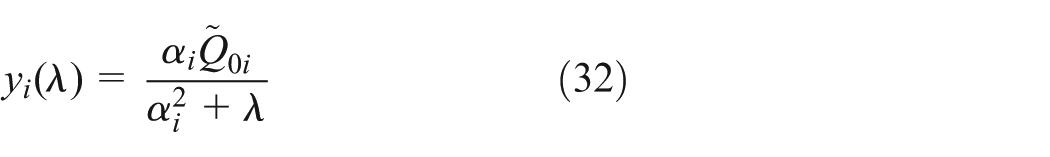
To determine the Lagrange parameter, we define

and seek a solution to

Reinforcement signal
The performance of an action
The repulsive potential function

where


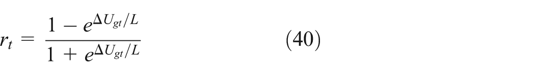
where L is the proportional coefficient and determined by the designer.
The attractive potential function

where

Based on the analysis mentioned above, the proposed RNQL algorithm can be summarized as follows:
RNQL algorithm
First, select the type of nodes (additive or RBF) and the corresponding activation function g and the hidden node number
Step 1: initialization phase: Initialize the learning using a small chunk of initial training data (a) Assign random input weights (b) Calculate the initial hidden layer output matrix
Step 2: Sequential Learning Phase: (a) Obtain the current state (b) Execute the action selected and obtain the next state of the mobile robot (c) Calculate numerical reward/penalty (d) Calculate the error term (e) Estimate and update the Q-value (f) Update
Remark 1
As OS-ELM, the proposed RNQL consists of two phases, namely, an initialization phase and a sequential learning phase. In the initialization phase, the initial weight
Remark 2
The obstacle avoidance task is achieved by an avoidance module and a goal-seeking module. The two modules independently apply the proposed RNQL to find the reference Q-value. But in the learning process, the state variables and the calculation of the reinforcement signal
Performance evaluation
In the section, the performance of the proposed RNQL algorithm is evaluated. First, the avoidance module and the goal-seeking module are independently trained using the RNQL algorithm under different simulation environments. Then, the trained modules are combined to navigate a robot to the goal without colliding the obstacles in the unknown environments. Note that all the environments are generated from the simulation software SimRobot (developed by the students and teachers in Department of Control and Instrumentation, Brno University of Technology).
For the purpose of comparison, the performance of the proposed RNQL algorithm is compared with the BPQL, which is commonly used in Yang et al., 8 Li et al., 9 Qiao et al., 11 and Ganapathy et al. 12 All the simulations are carried out in MATLAB 6.5 environment running in a Intel® Core™2 Quad CPU, 2.83 GHz.
Parameter configuration
The parameter values used for all the simulations are summarized in Table 1. For better understanding, the determination details of these parameters are described in the following.
Parameter values used for all of simulation studies.

L is a proportional coefficient for calculating the reinforcement signal
Performance comparison of avoidance module
In the avoidance module, the AMR is only required to move among many obstacles without collisions and without a specific target. Here, a simple simulation environment with four obstacles is designed to train the robot using the RNQL and then the generalization of the RNQL algorithm is verified in a more complex environment and a maze after the robot finishes its training. In the avoidance module, the state variable

The performance of the RNQL algorithm is evaluated from two criteria, namely continuous moving time without collision and training time. Here, we set up 50,000 s as the maximum continuous moving time that is the maximum simulation time. The comparison of the performance between the RNQL algorithm and BPQL algorithm is shown in Table 2.
Performance comparison between RNQL and BPQL algorithms for avoidance module.

RNQL: random neural Q-learning; BPQL: back-propagation Q-learning; STD: standard deviation.
For each algorithm, the results are averaged over 20 trials. The average training steps, the average training time, and the trial result that is the closest to the mean are shown in Table 2. From Table 2, it can be seen that the mobile robot trained by the proposed RNQL and BPQL algorithm can smoothly move 50,000 s after each trial. But the training steps in the RNQL are much lesser than those of BPQL. Besides, the training time of RNQL is much lesser that of BPQL. For the BPQL algorithm, because the learning parameters of the hidden nodes and the weights connecting the hidden nodes to the output nodes are all tuned in one training step, the speed of convergence for the algorithm is slow and the learning efficiency is low. It can be concluded that the robot trained by the proposed RNQL algorithm can move a longer time without collision after the same training steps compared with the BPQL algorithm. Furthermore, the shorter training time can be achieved by the proposed RNQL algorithm.
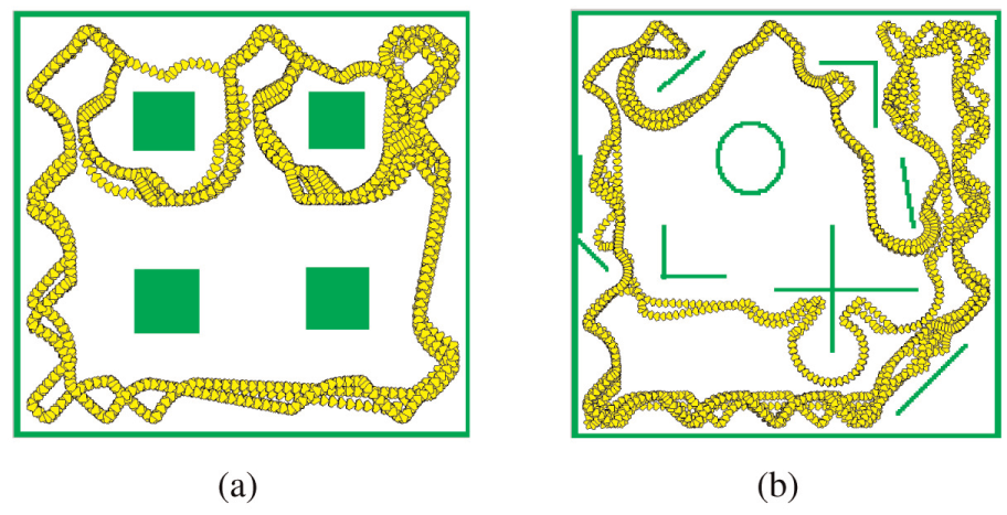
For the purpose of illustration, the results of the RNQL algorithm that is the closest to the mean are shown in Figure 5(a) and (b). It can be seen from Figure 5(b) that the robot successfully moves in a more complex environment no collision without being trained any more. Similarly, the training procedure and the testing result of the BPQL algorithm are shown in Figure 6(a) and (b) separately. In Figure 6(a), the mobile robot trained by the BPQL algorithm can move at least 50,000 s collisionless in the simple training environment after 6953 training steps. But in Figure 6(b), it can only move 6380 s without collision and then hit the obstacle in the complex environment.
Moving trajectories of the robot using RNQL: (a) training environment and (b) testing environment.

Moving trajectories of the robot using BPQL: (a) training environment and (b) testing environment.
The BPQL algorithm is based on the gradient-descent technique to training a SLFN. Gradient-based learning is generally time-consuming and is easy to stop at a local minimum if the unsuitable initial values of adjustable parameters are located far from an optimal solution. In Figure 6, the SLFN is trained by the BPQL algorithm and gets the sub-optimal solution. In this case, the global state–action mapping cannot be learnt. Thus, the robot collides with the edge of a block in testing environment, although it can move successfully without collision in training environment. In the proposed RNQL algorithm based on the ELM algorithm, the problem of training a SLFN is converted to obtain a solution of a linear system with the random parameters of the input layer. The smallest least-square training error can be reached by the Moore–Penrose generalized inverse approach. In Figure 5, the proposed algorithm may find the optimal solution compared with the BPQL algorithm. Thus, it can extend to move in the complex environments successfully.
To further evaluate the performance of the proposed RNQL algorithm, a more complex environment, that is, a maze is applied here. Figure 7(a) shows that the mobile robot trained by RNQL algorithm successfully moves at least 50,000 s without collision in the maze environment. As shown in Figure 7(b), the mobile robot trained by the BPQL algorithm can only move 9157 s without collision and then hit the obstacle in the environment.

Moving trajectories of the robot in a maze: (a) trained by RNQL and (b) trained by BPQL.
Therefore, from Figures 5–7, it can be concluded that the proposed RNQL algorithm has better generalization ability and higher learning efficiency than the BPQL, where the mobile robot trained by the proposed algorithm can move without collision in different unknown environments without being trained any more.
Besides, in the proposed RNQL algorithm, a different initialization phase from that of OS-ELM is presented to estimate the initial value of the output weights for improving the learning performance. To verify this point, the performance between the proposed initialization method and the original one is compared and shown in Table 3, from which it can be observed that the proposed initialization estimation method has faster convergence speed with the lesser training steps and training time. Also it achieves better generalization ability without collision in the complex environments, whereas the original initialization phase in the OS-ELM moves 41,797 s without collision and then hits the obstacle in the complex environment.
Performance comparison between the proposed initial phase and the original one.
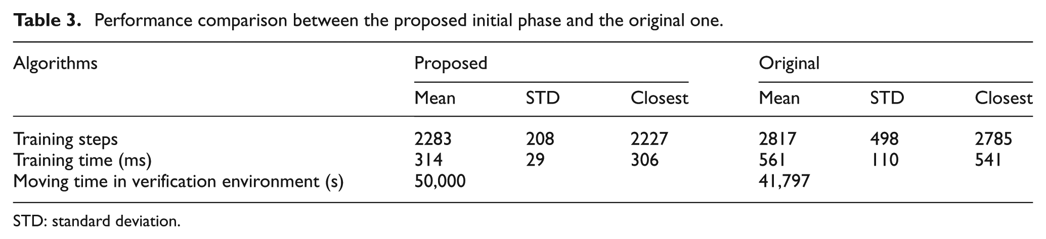
STD: standard deviation.
Performance comparison of goal-seeking module
In the goal-seeking module, the AMR is trained to move to a target point without any obstacles. In this module, the state variable


where
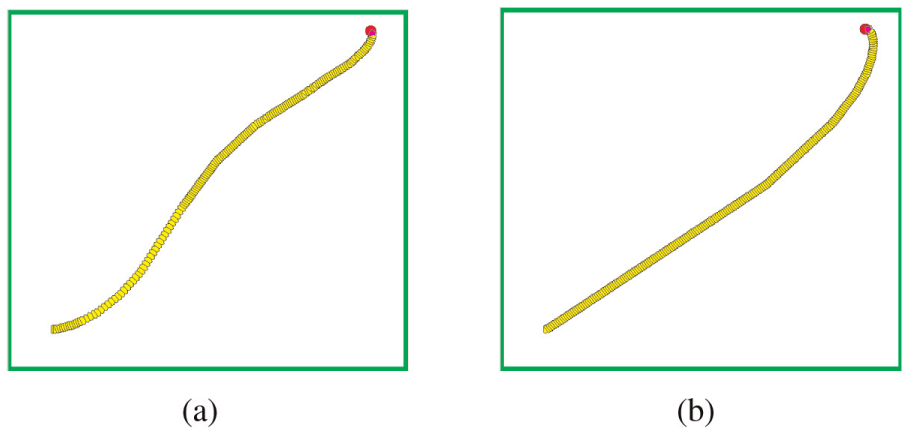
First, a simulation environment without obstacles as shown in Figure 8(a) is designed to train the robot using the RNQL where the red circle dot is the target point and the initial position is set as (49, 52, 0). The numerical comparison between the RNQL algorithm and BPQL algorithm is shown in Table 4. For each algorithm, the results are averaged over 20 trials. The average training steps, the average training time, and the result of trial that is the closest to the mean are shown in Table 4. The moving trajectories of the robot from the initial training point to the goal are shown in Figure 8. That is the result of trial which is the closest to the mean. From the table, it can be observed that the lesser training steps and training time are required by the RNQL algorithm than those of the BPQL algorithm. This means that the RNQL algorithm has faster convergence speed than the BPQL algorithm.

Moving trajectories of the robot from the training start position (49, 52, 0) to the goal: (a) RNQL and (b) BPQL.
Performance comparison of RNQL algorithm and BPQL algorithm for goal-seeking module.

RNQL: random neural Q-learning; BPQL: back-propagation Q-learning.
An additional four different initial positions are applied to verify the performance of the goal-seeking behavior module. Figures 9–12 show the moving trajectories from the four different initial positions to the goal based on the RNQL and BPQL algorithms. As shown in these figures, although the initial positions are varied, the robot is able to move to the target using the two learning algorithms above. The numerical performance comparison of the moving steps based on the RNQL algorithm and BPQL algorithm is shown in Table 5. From the table, it can be observed that the lesser moving steps can be obtained by the RNQL algorithm than those of the BPQL algorithm. This means that the robot trained by the RNQL algorithm can arrive at the goal faster than the one trained by the BPQL algorithm.
Moving trajectories of the robot from the position (41, 38, 0) to the goal: (a) RNQL and (b) BPQL.

Moving trajectories of the robot from the position (248, 157, 0) to the goal: (a) RNQL and (b) BPQL.

Moving trajectories of the robot from the position (106, 147,

Moving trajectories of the robot from the position (97, 108,
Verification performance comparison of RNQL and BPQL algorithms for goal-seeking module.

RNQL: random neural Q-learning; BPQL: back-propagation Q-learning.
Simulation of obstacle avoidance
In the proposed obstacle avoidance method, once the network parameters for the two behavior modules are completely built through the RNQL algorithm, the two behaviors will be combined so that the robot arrives at the given goal position without colliding with obstacles. In this section, the avoidance module and goal-seeking module are now combined to navigate a robot to reach the target position. When the robot navigates in a certain environment, one of the two behaviors must be selected at each action step in order to accomplish its goal. This is performed by a switching function expressed by equation (9). First, the robot is required to move to the target position in an environment with four obstacles under four different initial positions as shown in Figure 13.
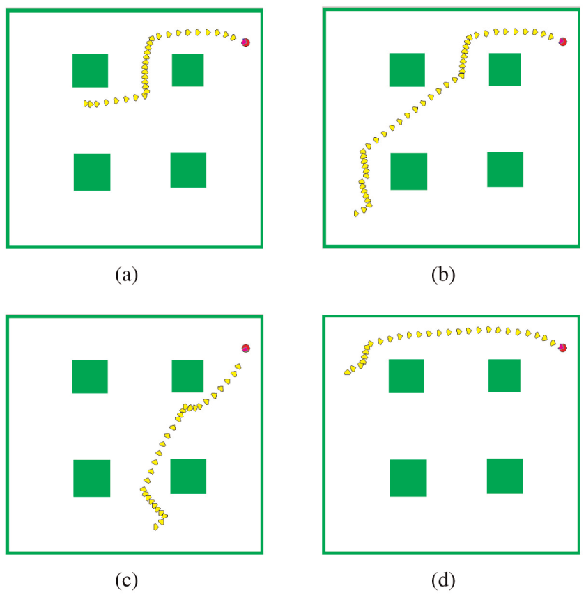
Mobile robot moves to a target from different initial position without collision in the simple environment: (a) (96, 176, 0); (b) (31, 32, 0); (c) (180, 41, 0) and (d) (28, 219, pi/2).
From the figure, it can be observed that whatever the initial position of the robot is, the robot can arrive at the target position in a smooth path while keeping a certain distance with obstacles. Also a complex environment with many different obstacles as depicted in Figure 14 is further used to verify the obstacle avoidance performance of a trained robot by reaching the specific target. Besides, a more complex maze environment with different initial and target positions as shown in Figures 15 and 16 is applied here to evaluate its performance. From the figures, one can note that the trained robot can successfully move from different start points to the different goals in complex environments. Besides, the results of the BPQL algorithm for the three verification environments are given in Figure 17 for the purpose of comparison. From the figure, it can be seen that the robot is navigated successfully to the target in the simple environment while it fails in the complex environments. It can be concluded that the proposed obstacle avoidance strategy has good generalization ability and also has good ability to adapt to a new environment.

Mobile robot moves to a target from different initial position without collision in the complex environment: (a) (27, 28, 0); (b) (48, 165, 0); (c) (30, 338, pi/2) and (d) (256, 55, pi/2).

Mobile robot moves to a target closer from the obstacles from different initial position in a maze: (a) (25, 327,-pi/2); (b) (26, 58, pi/2); (c)(101, 237, pi/2) and (d) (253, 23, pi/2).

Mobile robot moves to a target farer to the obstacles from different initial position in a maze: (a) (25, 327, -pi/2); (b) (26, 58, pi/2); (c) (101, 237, pi/2) and (d) (253, 23, pi/2).

Moving trajectories of BPQL from different initial position in three verification environments: (a) (96, 176, 0); (b) (31, 32, 0); (c) (27, 28, 0); (d) (48, 165, 0); (e) (25, 327, -pi/2) and (f) (26, 58, pi/2).
Conclusion
In this article, a simple and efficient learning strategy for the AMR’s obstacle avoidance problem in uncertain environments has been proposed. The core avoidance and goal-seeking modules in the strategy are trained by a novel RNQL algorithm where the SLFN is used as a Q-function approximator to estimate the Q-value. In the proposed RNQL algorithm, the parameters of the SLFN are tuned by the OS-ELM algorithm. However, different from the original OS-ELM, the initial output weights of the SLFN are estimated subjected to a quadratic inequality constraint. Performance of RNQL is compared with BPQL algorithm on obtaining the optimal learning policies for the avoidance and goal-seeking modules. The results indicate that the RNQL produces better learning performance in terms of convergence speed, training time, and generalization ability. The proposed learning strategy can effectively navigate the AMR to arrive at the goal without colliding with the obstacles in unknown environments.
The proposed algorithm is a general way to guide the mobile robot to reach a target. But the effectiveness of the presented algorithm depends on some sensing information, that is, the position of the robot, the coordinate of the goal, and the distances between the target and the obstacles. Therefore, while the mobile robot system has the positioning and obstacle detection sensors, the proposed algorithm is an effective method for guiding the robot to reach the destination. In the case of lacking the positioning sensors, the proposed algorithm can also lead the robot to reach the goal if the target can be identified via some specific sensors. For example, the mobile robot can detect obstacles and the goal by cameras. However, the mobile robot will move randomly when the target is out of the detection range of the camera. If the robot enters the target detection range, it moves toward the target. This will cause a longer navigation time. Moreover, a larger safe distance between the target with the nearest obstacles is required. This can ensure enough space for the robot to move to the target from different initial positions. If the safe distance is smaller, the avoidance module plays a main role. The robot wanders around the target and cannot arrive at the target. The determination of the minimum safe distance is not an easy task since it depends on many factors. We will discuss it in our future work.
Footnotes
Academic Editor: Pak Wong
Declaration of conflicting interests
The author(s) declared no potential conflicts of interest with respect to the research, authorship, and/or publication of this article.
Funding
The author(s) disclosed receipt of the following financial support for the research, authorship, and/or publication of this article: This work is funded in part by National Natural Science Foundation of China (Grant No. 61403300), National Science Council of ShaanXi Province (Grant No. 2014JM8337), and the Fundamental Research Funds for the Central Universities.