An Analytical Approach to Avoid Obstacles in Mobile Robot Navigation

Abstract

A nonlinear supervised globally stable controller is proposed to reactively guide a mobile robot to avoid obstacles while seeking a goal. Whenever the robot detects an object nearby, its orientation is changed to be aligned with the tangent to the border of the obstacle. Then, the robot starts following it, looking for a feasible path to its goal. The supervisor is responsible for deciding which path to take when the robot faces some particular obstacle configurations that are quite difficult to deal with. Several simulations and experiments were run to validate the proposal, some of which are discussed here. To run the experiments, the proposed controller is programmed into the onboard computer of a real unicycle mobile platform, equipped with a laser range scanner. As for the simulations, the models of the same experimental setup were used. The final conclusion is that the nonlinear supervised controller proposed to solve the problem of avoiding obstacles during goal seeking has been validated, based on the theoretical analysis, and the simulated and experimental results.

1. Introduction

When a mobile robot is seeking a goal, it is supposed to avoid obstacles along its path. It should also evaluate the distance to the goal, to locally define how to get closer to it. Hence, the robot should know the goal coordinates, related to its own frame, and the arriving angle (if specified). Thus, the objective is to control the robot movement such that the error between its current position and its goal becomes as small as possible, after leaving all obstacles behind, respecting the specified arriving angle (the orientation after reaching the goal).

Several approaches have been proposed to guide the robot to accomplish such a task. Some of them include a path-planning step, performed over a previously known map of the environment, before starting the robot navigation. This is also called global path-planning. Therefore, such strategies are based on the deliberative paradigm. In other words, the mobile robot has a global map of the environment surrounding it, then the control algorithm plans the actions to accomplish the desired task based on such a map [1]. The approaches reported in [2–5] are good examples of deliberative ones.

However, a weakness of such a class of approaches is that after planning the entire path, the environment cannot change further. If that happens (for instance, an obstacle not included in the environmental map appears), free-of-collision navigation is no longer guaranteed.

Other approaches to avoid obstacles are based on the reactive paradigm [1], whose basic assumption is that the robot has no a priori knowledge about the environment surrounding it. It simply reacts to such an environment according to its perception of it. As a consequence, reactive navigation demands a suitable sensing system and also much less computation for working with local information (the presence/absence of an obstacle close to the robot). Environment changes are no longer a problem: the robot perceives the changes and reacts to them (for instance, the presence of a static obstacle that was not in the environment in a previous navigation). Therefore, reactive navigation is more suitable to weakly structured environments, while deliberative navigation is more suitable to strongly structured environments. Edge detection [6] and potential fields [7] are classical examples of reactive navigation strategies (more recent examples of reactive navigation are reported in [8–11]).

To overcome the problem of not being able to deal with unpredicted obstacles, some deliberative approaches [4, 5, 12] temporarily change the planned path, reacting to the presence of an obstacle. Therefore, they would be better classified as hybrid approaches [1], involving both deliberative and reactive paradigms.

In such a context, this paper revisits the problem of obstacle avoidance in mobile robot navigation, and proposes a strictly reactive, simple and fast-to-compute approach, hereinafter referred to as tangential escape, to guide the robot to reach a pre-defined goal after leaving behind any obstacle appearing in its path. In essence, such an approach is quite different to other previously proposed approaches to performing the same task, as it will become clear. For instance, it demands a far simpler feature extraction, in terms of the sensorial data, compared to the approach proposed in [8]: our proposal requires just the knowledge of the minimum robot-obstacle distance. Compared to the approach proposed in [13], the advantage of the approach proposed here is that no decision-tree is computed, thus allowing a faster reaction in the presence of obstacles. Compared to the approach proposed in [11], derived from the potential field method, an additional random force is adopted there to allow the robot to escape from the obstacle, whereas in our strategy this is performed by a supervisor added to the controller.

On the other hand, the approach here discussed is conceptually similar to the tangent bug algorithm [14, 15]: both are globally convergent and assure that the path followed by the robot in the free-space is optimum (it moves along the shortest path linking its current position and the goal, when well-oriented with respect to it). However, the implementation proposed here is quite different: a single supervised nonlinear Lyapunov-based controller is adopted to implement the behaviours “to navigate towards the goal” and “to follow the obstacle boundary” [10, 14]. The global convergence is also guaranteed in our approach, since the control system implemented is proven to be globally asymptotically stable in the absence of obstacles and is able to leave all obstacles behind (see Subsection 2.2 and Section 3, respectively). Therefore, after leaving all obstacles behind, it is guaranteed that the robot will reach the goal (supposing it can be reached). In addition, the use of the Lyapunov theory to design such a controller also guarantees that the robot moves towards the goal following the least-energy path, in the absence of obstacles.

As for the version of the tangential escape published in [16], this manuscript describes all aspects of the technique, whereas the first published version discusses just the basic idea. In terms of novelty, most content of Section 3, the simulations and most experiments of Section 4 are being presented for the first time. Actually, using the version of the tangential escape strategy published in [16], the simulations and the most difficult experiments reported in Section 4 would not attain the same result, for that version did not deal with the possibility that the robot can get trapped in the obstacle. Therefore, this version of the tangential escape algorithm is complete, whereas the one in [16] is the first step in the method.

To describe and validate the tangential escape approach, the paper is hereinafter split in four sections. The kinematic model of the mobile robot and a nonlinear controller able to guide it to the goal in the absence of obstacles are presented in Section 2. Section 3 describes the implementation of the tangential escape approach through a nonlinear control system, using the range measurements provided by a laser scanner onboard the robot. Notice that any other range sensor could be used instead of a laser range finder (the proposed approach relies on the range measurements, not on the range sensor). However, as the laser scanner allows getting range measurements with quite a good angular resolution, it was adopted here. The results of the simulations and real experiments run using such a control system are presented and discussed in Section 4. Finally, Section 5 highlights the main conclusions of the work.

2. Seeking the Goal in Free-space

The strategy we propose encompasses two subtasks the robot should accomplish: reduce its distance to the goal, if there are no obstacles inside a semi-circle of radius d_obs in front of it, and change its current orientation to avoid the closest obstacle, if there are obstacles inside the same semi-circle. In the second case, after leaving the obstacle behind the robot resumes the first subtask, and the distance robot-goal is continuously reduced. As a result of such a combination, the robot reaches its goal after leaving all obstacles behind. In addition, if the robot should assume a given orientation after reaching the goal, its final orientation is corrected, while keeping its position. Such a strategy is illustrated by the basic flow diagram of Figure 1, which will be analysed in depth in the sequel.

Figure 1.

Flow diagram of the proposed strategy.

To implement the proposed approach, such behaviours are embedded in a nonlinear control system having two nested loops. The inner one is in charge of reducing the distance robot-goal in the absence of obstacles, whereas the outer one is responsible for steering the robot away from the obstacle closest to it. In this section, the inner control loop is discussed: a controller to guide the robot to reach the goal is proposed, and the equilibrium of the closed-loop control system thus implemented is proven to be globally asymptotically stable. Thus, the robot will reach the goal after leaving all obstacles behind, assuring the global convergence [14].

2.1 The Kinematic Model of the Robot

The mobile robot used in the experiments here reported is a differential drive platform, whose kinematic model is

$\left[\begin{array}{c}\stackrel{.}{x}\\ \stackrel{.}{y}\\ \stackrel{.}{\psi }\end{array}\right]=\left[\begin{array}{cc}\cos \psi & -a\sin \psi \\ \sin \psi & a\cos \psi \\ 0& 1\end{array}\right]\left[\begin{array}{c}u\\ \omega \end{array}\right],$

where u and ω are, respectively, the linear and angular velocities, x and y are the current coordinates of the point of interest (whose position should be controlled), ψ is the robot orientation with respect to the x-axis of the global frame 〈o〉, and a is the distance from the point whose position is being controlled (the position of the laser scanner) to the middle of the virtual axle linking the driven wheels (see Figure 2). The mathematical description of the navigation towards the goal in an environment free of obstacles, in polar coordinates, is given by [17]

$\begin{array}{l}\stackrel{.}{H}=\left[\begin{array}{c}\stackrel{.}{\rho }\\ \stackrel{.}{\alpha }\\ \stackrel{.}{\theta }\end{array}\right]=\left[\begin{array}{cc}-\cos \alpha & -a\sin \alpha \\ \frac{\sin \alpha }{\rho }& -a\frac{\cos \alpha }{\rho }-1\\ \frac{\sin \alpha }{\rho }& -a\frac{\cos \alpha }{\rho }\end{array}\right]\left[\begin{array}{c}u\\ \omega \end{array}\right]+\\ \hspace{0.17em}\hspace{0.17em}\hspace{0.17em}\hspace{0.17em}\hspace{0.17em}\hspace{0.17em}\hspace{0.17em}\hspace{0.17em}\hspace{0.17em}\hspace{0.17em}\hspace{0.17em}\hspace{0.17em}\hspace{0.17em}\hspace{0.17em}\hspace{0.17em}\underset{=0}{\underbrace{\left[\begin{array}{c}{\stackrel{.}{\mathrm{x}}}_{\mathrm{d}}\cos \theta +{\stackrel{.}{\mathrm{y}}}_{\mathrm{d}}\sin \theta \\ -{\stackrel{.}{\mathrm{x}}}_{\mathrm{d}}\sin \theta +{\stackrel{.}{\mathrm{y}}}_{\mathrm{d}}\cos \theta \\ -{\stackrel{.}{\mathrm{x}}}_{\mathrm{d}}\sin \theta +{\stackrel{.}{\mathrm{y}}}_{\mathrm{d}}\cos \theta \end{array}\right]}}=Kv,\end{array}$

(1)

Figure 2.

The mobile robot seeking the goal 〈g〉.

where p is the distance robot-goal (the goal is marked as 〈g〉 in Figure 2, and its coordinates in 〈o〉 are defined by the user). The direction of movement is always orthogonal to the virtual axle, and causes the orientation error α with respect to the goal position. The angle θ defines the orientation desired when the robot reaches the goal, and α + ψ = θ (see Figure 2). The inertial system of coordinates shown in the figure, 〈o〉, corresponds to the robot initial position. Notice that the rightmost term of (1) is null, because only position control is considered in this work, meaning that the goal is static, i.e., ẋ_d = ẏ_d = 0.

Notice that the robot deals with a local polar depth map, similar to the one used in [18]. Notice also that ρ cannot be zero, because this would make α and θ undefined. Thus, the robot is considered in the goal when ρ ≤ δ, where δ is an arbitrarily small positive value (hereinafter 30 mm).

2.2 Position Control in the Free-Space

From Figure 2 one can see that the robot can be effectively controlled by suitably controlling the values of u and ω. Then, a control system aiming at making ρ → 0 and α → 0 is proposed. A control law that guarantees the additional condition θ → θ_d, after getting the conditions ρ → 0 and α → 0, if necessary, is discussed in the next subsection.

Therefore, the objective here is to make the state vector H = [ρ α]^T go asymptotically to zero, from any initial value. To design a controller guaranteeing that, the Lyapunov candidate function

$V=\frac{1}{2}{H}^{\mathrm{T}}H>0$

is adopted, and the control law designed should make the first temporal derivative of V,V̇ = H^TḢ, be negative for all nonzero values of H to guarantee the stability of the closed-loop system (to guarantee that H → [0 0]^T).

Taking into account the kinematic model in (1), one gets

$\stackrel{.}{V}={\stackrel{.}{H}}^{T}Kv$

which is negative for any nonzero value of H for the control law

$v=K^{-1}({\stackrel{.}{H}}_d-\kappa \tanh H)$

(2)

where κ is a diagonal positive definite matrix. Therefore, considering Ḣd = 0 (because in position control the goal is static),

$\stackrel{.}{V}=-H^T\kappa \tanh H<0$

thus demonstrating the global asymptotic convergence of H→0, meaning that the robot will always reach its goal in the absence of obstacles. It should be observed that when the robot reaches the goal it stays there, because the values of u and ω become zero, as one can see from

$\left[\begin{array}{c}\mathrm{u}\\ \omega \end{array}\right]=\left[\begin{array}{cc}{\mathrm{u}}_{\max }& 0\\ 0& {\omega }_{\max }\end{array}\right]\left[\begin{array}{cc}\frac{\rho +\alpha \cos \alpha }{\mathrm{a}+\rho \cos \alpha }& \frac{\mathrm{a}\rho \sin \alpha }{\mathrm{a}+\rho \cos \alpha }\\ \frac{\sin \alpha }{\mathrm{a}+\rho \cos \alpha }& 1-\frac{\mathrm{a}}{\mathrm{a}+\rho \cos \alpha }\end{array}\right]\left[\begin{array}{c}\tanh \rho \\ \tanh \alpha \end{array}\right],$

(3)

which is obtained from (2), when Ḣ_d = 0.

To complete the stability analysis, it is important to check the behaviour of the angle θ when the robot reaches the goal. Knowing that ψ̇=ω and that the system is asymptotically convergent, ω → 0 when the robot reaches the goal. Taking into account that (tanh ρ)/p → 1 when ρ → 0, it results that ψ̇=θ̇→0 when t → ∞. Therefore, θ = ψ tends to a bounded value, showing that the robot reaches the goal with a well-behaved arriving angle, although not defined by the designer.

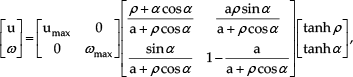
The function tanh is used to saturate the values of u and ω at the maximum values, u_max and ω_max, obtained from the robot data sheet. Such saturation is adopted to prevent the possibility that the physical actuators of the mobile robot saturate, which would occur in the case of a control signal of large magnitude.

The control system proposed to guide the robot to reach the goal in the absence of obstacles is illustrated in Figure 3. There X _d =[x_d y_d] ^T defines the goal position, X = [x y] ^T defines the current robot position, obtained through the robot odometry (as well as the angle ψ), $\tilde{\mathrm{x}}={[\tilde{\mathrm{x}}\hspace{0.17em}\hspace{0.17em}\tilde{\mathrm{y}}]}^{\mathrm{T}}={[({\mathrm{x}}_{\mathrm{d}}-\mathrm{x})({\mathrm{y}}_{\mathrm{d}}-\mathrm{y})]}^{\mathrm{T}}$ , so that $\rho =\sqrt{{\tilde{\mathrm{x}}}^2+{\tilde{\mathrm{y}}}^2}$ and $\theta =arctan\frac{\tilde{\mathrm{y}}}{\tilde{\mathrm{x}}}$ .

Figure 3.

The control system in charge of guiding the robot to the goal in the absence of obstacles.

2.3 Orientation Control in the Goal

After reaching the goal position, the robot can be badly oriented to perform some specific task, such as grasping an object using an onboard end-effector, for instance. In this case, it is necessary to control just the angle ψ, not allowing any additional displacement (taking advantage of the fact that the mobile platform is a unicycle one). To do that, it is now designed an additional controller to impose a suitable angular velocity ω to the robot, while keeping its linear velocity u null (to keep it in the goal).

From Figure 2 one can notice that θ = ψ_d, so that α =ψ_d-ψ=ψ˜ is the final orientation error. Thus, for a constant final orientation it results that $\stackrel{.}{\stackrel{~}{\psi }}=-\stackrel{.}{\psi }=\stackrel{.}{\alpha }$ is the model of the robot when manoeuvrearound to correct the orientation without moving ahead or back. In such a case, one can choose the Lyapunov candidate function

$\mathrm{V}\left(\alpha \right)=\frac{1}{2}{\alpha }^2,$

(4)

whose first time derivative is

$\stackrel{.}{\mathrm{V}}\left(\alpha \right)=\alpha \stackrel{.}{\alpha }=\tilde{\psi }\left(-\omega +\mathrm{u}\frac{\sin \tilde{\psi }}{\rho }-a\omega \frac{\cos \tilde{\psi }}{\rho }\right).$

(5)

Now, imposing that

$\{\begin{array}{l}\mathrm{u}=0\hfill \\ \omega ={\omega }_{\max }\tanh \tilde{\psi },\hfill \end{array}$

(6)

with ω_max > 0, and remembering that the robot is already in the goal, or ρ ≤ δ, one gets

$\stackrel{.}{\mathrm{V}}\left(\alpha \right)=-{\omega }_{\max }\tilde{\psi }\tanh \tilde{\psi }\left(1+\frac{\mathrm{a}}{\delta }\cos \tilde{\psi }\right),$

(7)

which is negative definite if |ψ˜|<π/2. Thus, the orientation error ψ˜ converges asymptotically to zero, and hence ψ converges asymptotically to ψ_d, the desired value.

2.4 Stability During the Switching of the Control Systems

After reaching the goal, the robot should orientate itself to reach the desired final pose. Therefore, it is necessary to switch from the position controller to the orientation one, in order to correct the robot orientation on arrival. In such a case, the stability of the control system during the switching should also be guaranteed. This is done using the direct extension of the theorem of Lyapunov, which guarantees the stability during the switching when the individual controllers are designed using the same Lyapunov candidate function [19].

In the present case, as α = ψ˜, it is straightforward to demonstrate that (2) and (4) represent the same Lyapunov function. Therefore, the stability during the switching from the position error controller to the orientation controller is guaranteed.

To conclude this section, it is worth mentioning that one could design a control law involving α, ρ and θ simultaneously [17], instead of using the strategy of correcting the arrival angle only after reaching the goal.

3. The Proposed Approach

A nonlinear controller to guide the robot while avoiding obstacles is now proposed. The strategy adopted to design such a controller consists in choosing an escape path that is tangent to the obstacle border, in a way quite similar to the navigation adopted by human beings in unknown environments. Such a controller also includes a supervisor, which is in charge of changing the robot orientation right after the occurrence of some specific situations, allowing the vehicle to escape of typical local minima, as discussed in the sequel.

The proposed controller uses the scheme discussed in Section 2 for reducing the distance robot-goal. However, the goal position is redefined whenever an obstacle is detected at a distance smaller than or equal to d_obs from the robot. Thus, d_obs defines the obstacle avoidance zone shown in Figure 4, and when the robot enters such a zone it should start an evasive manoeuvre. In the same figure, d_min is the smallest robot-obstacle distance, correspondent to a certain range scan. In the presence of an obstacle d_min ≤ d_obs a temporary target, X _v , called virtual goal, is created, whose position is obtained from the position of the real goal, X _d , through a rotation matrix. Notice that the line linking the point being controlled and the virtual goal is tangent to the border of the detected obstacle, as shown in Figure 4.

Figure 4.

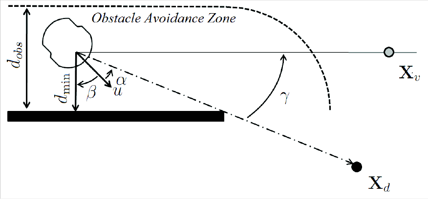
The tangential escape approach. Notice that $0<\beta <\frac{\pi }{2}$ , and α > 0, resulting in γ < 0.

The rotation angle γ, which defines the rotation matrix that creates the virtual goal, is obtained from the set of range measurements provided by an onboard rangefinder. To define γ, it is necessary to know β, which defines the position of the closest obstacle. After each range scan, the proposed system checks if there is at least one distance d ≤ d_obs, and the angle correspondent to such a value is the angle β. The laser scanner here adopted as the rangefinder delivers range measurements for angles in the range [0°, 180°], in steps of 1°. Such angles are mapped to the range [–90°, +90°], so that β < 0 when the obstacle is to the right of the robot and β > 0 when the obstacle is to the left. Given β one gets

$\gamma =\{\begin{array}{c}-90°+\beta -\alpha \hspace{0.17em}\hspace{0.17em}\mathrm{if}\beta \ge 0\\ +90°+\beta -\alpha \hspace{0.17em}\hspace{0.17em}\mathrm{if}\beta <0\end{array}$

(8)

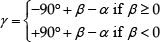
where α > 0 when the goal is at the right side of the axis of movement of the robot (see Figure 4). Notice that in Figure 4, the angle γ is positive, causing the rotation of the real goal to the left, considering the axis of movement of the robot.

As the robot navigates in a plane, the angle γ is used to get

$X_{\mathrm{v}}=\left[\begin{array}{cc}\cos \gamma & -\sin \gamma \\ \sin \gamma & \cos \gamma \end{array}\right]X_{\mathrm{d}},$

(9)

where X_d and X_v are, respectively, the position of the real goal (desired) and the virtual goal (temporary). Having the coordinates of X_v the position controller guides the robot to the new goal, following the tangent to the obstacle border. Notice that in the absence of obstacles there is no change in the position of the real goal (γ = 0°), and the robot continues getting closer to it.

It should be emphasized that this strategy is different from the one presented in [20], for instance, in the sense that there is no fictitious forces characterizing the interaction robot-environment. Thus, no impedance parameters should be selected for the present strategy, like in [20], making it easier to set the system parameters. The designer just has to define the distance d_obs that characterizes the obstacle avoidance zone shown in Figure 4. This is an important characteristic of the strategy here proposed, because the system based on fictitious forces may cause the robot to get stuck in certain situations [16, 21].

The control system proposed to implement the tangential escape approach is depicted in Figure 5, where u, ω, ψ, X_d and X_v are defined in Subsection 2.2, whereasd represents the set of range measurements provided in each scan of the laser range sensor, and γ is the rotation angle. Notice that the block pose controller is active all the time, i.e., the robot does not stop to manoeuvre in order to deviate from the obstacle. Based on such a diagram, and taking into account the asymptotic stability of the pose controller, one can conclude that after leaving all obstacles behind the robot always reaches its goal, unless it is not reachable.

Figure 5.

Block diagram of the control system based on the tangential escape approach.

To describe the tangential escape strategy a little further, the following subsections present particular cases of obstacle configurations that the robot can face during navigation, highlighting how the system proposed here deals with each one.

3.1 Dealing with Corner-like Obstacles

There are situations in which the robot should perform more aggressive manoeuvres in order to overcome an obstacle. One such situation is when it should overcome a corner-like obstacle, as in the case of L-, V- or U-shaped obstacles. This situation is illustrated in Figure 6, where the real goal is below the horizontal part of the L-shaped obstacle.

Figure 6.

Changing the tangential escape approach to take into account corner-like obstacles.

In these cases, the value of the angle γ in (8) does not guarantee that the robot will escape the obstacle. Actually, after turning around according to the angle γ, in Figure 6, the robot faces the vertical part of the obstacle, and should continue turning around. To make such a manoeuvre faster, we change the value of γ in (8) to

$\gamma =\{\begin{array}{c}-180°+\beta -\alpha \hspace{0.17em}\hspace{0.17em}\mathrm{i}\mathrm{f}\beta \ge 0\\ +180°+\beta -\alpha \hspace{0.17em}\hspace{0.17em}\mathrm{i}\mathrm{f}\beta <0\end{array}$

(10)

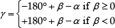
whenever the distances d_90° (the range measurement correspondent to the angular position β − 90°, if β ≥ 0, or β + 90°, if β < 0 - see Figure 6) and d_min are simultaneously less than d_obs (90° is added to γ, with the same signal).

In addition, as the robot should perform a strong turn around manoeuvre, it is also necessary to change how the virtual goal is defined, to guarantee that u is low enough to minimize the risk of a collision during the evasive manoeuvre (cautious navigation). From (3), a possible solution to reduce the value of u is to reduce the value of ρ = ‖X_v – X|^1/2 during obstacle avoidance. Our proposal is to use

$X_v=\left[\begin{array}{cc}\cos \gamma & -\sin \gamma \\ \sin \gamma & \cos \gamma \end{array}\right]\left[\begin{array}{c}{\mathrm{d}}_{\min }\cos \theta \\ {\mathrm{d}}_{\min }\sin \theta \end{array}\right]$

(11)

as the virtual goal, instead of (9), which corresponds to considering the virtual goal closer to the robot, in the same direction. The result is that the robot turns around with a lower linear velocity, thus reducing the risk of collision during the evasive manoeuvre.

3.2. Dealing with Concave Obstacles

Another particular situation that deserves special attention is when the robot is badly oriented with respect to the goal. A good example is when the robot finishes following one side of a U-shaped obstacle, as illustrated by the darker sketch in Figure 7. The robot navigates from the white sketch straightforwardly to the real target, entering the U-shaped obstacle. When it gets close to the bottom of the U-shaped obstacle it turns left and follows the obstacle border. When it gets close to the upper part of the U-shaped obstacle it turns left again, according to (9) or (11), and follows the side of the U-shaped obstacle, until reaching the position correspondent to the darker robot sketch. In such a position, the orientation error α illustrated in the figure shows that the robot is badly oriented with respect to the real goal.

Figure 7.

Turning around 90° to overcome the obstacle extremity.

After getting rid of the obstacle, the robot could rotate to the left, to resume the navigation towards the real goal, getting trapped inside the U-shaped obstacle (a typical case of local minimum). To escape from such a local minimum, an auxiliary flag P_obs is created, to indicate the presence (or absence) of an obstacle. After getting a new scan of the laser rangefinder, P_obs is set to 1 if at least one range measurement is less than d_obs, and reset to 0 if all the range measurements in a laser scan are greater than d_obs. Analysing the transition of P_obs, it is possible to determine when the robot faces an obstacle (a positive-edge transition) or leaves it behind (a negative-edge transition). Notice that if the robot follows the obstacle border, at least one range measurement in a laser scan will be less than d_obs, thus not causing new negative-edge transitions in P_obs before finishing following the obstacle border.

After overcoming the obstacle, to avoid getting trapped the robot mimics human behaviour when navigating in an unknown environment containing walls: it rotates over the obstacle extremity. When the flag P_obs is reset the value of |α| is checked: if it is greater than 90°, as depicted in Figure 7, the robot manoeuvres in order to contour the extremity of the U-shaped obstacle (following the dashed line of Figure 7). This is done by creating a temporary goal and using the tangential escape approach to navigate towards it, as shown in Figure 8. Such new temporary goal ([x_tg y_tg]^T) is defined as

$\left[\begin{array}{c}{\mathrm{x}}_{\mathrm{t}\mathrm{g}}\\ {\mathrm{y}}_{\mathrm{t}\mathrm{g}}\end{array}\right]=\{\begin{array}{c}\left[\begin{array}{c}\mathrm{x}\\ \mathrm{y}\end{array}\right]+{\mathrm{d}}_{\min }\left[\begin{array}{cc}-\sin \psi & \cos \psi \\ \cos \psi & \sin \psi \end{array}\right]\left[\begin{array}{c}1\\ 1\end{array}\right]\hspace{0.17em}\hspace{0.17em}\hspace{0.17em}\mathrm{i}\mathrm{f}\beta \ge 0\\ \left[\begin{array}{c}\mathrm{x}\\ \mathrm{y}\end{array}\right]+{\mathrm{d}}_{\min }\left[\begin{array}{cc}\sin \psi & \cos \psi \\ -\cos \psi & \sin \psi \end{array}\right]\left[\begin{array}{c}1\\ 1\end{array}\right]\hspace{0.17em}\hspace{0.17em}\hspace{0.17em}\mathrm{i}\mathrm{f}\beta <0,\end{array}$

(12)

Figure 8.

Flow diagram of the whole tangential escape algorithm.

where X = [x y]^T corresponds to the current robot position referred to the inertial frame, ψ is its current orientation, d_min is the minimum distance robot-obstacle in the range scan obtained right before resetting P_obs, and β is the angle correspondent to d_min. Then, the robot starts seeking this temporary goal, using the position controller depicted in Figure 3. However, if it detects an obstacle during this temporary goal-seeking, it resumes its original goal and stops seeking the temporary one.

Otherwise, after reaching the temporary goal the robot corrects its orientation, in order to get oriented as in the intermediary grey robot sketch in Figure 7. Such a correction is performed using the orientation controller discussed in Subsection 2.3, for which the desired orientation angle is

${\psi }_{\mathrm{t}\mathrm{g}}=\{\begin{array}{c}\psi +90°\hspace{0.17em}\hspace{0.17em}\mathrm{i}\mathrm{f}\beta \ge 0\\ \psi +90°\hspace{0.17em}\hspace{0.17em}\mathrm{i}\mathrm{f}\beta <0,\end{array}$

(13)

where ψ is the robot orientation just before resetting P_obs. After this re-orientation, the robot is in the temporary goal and better oriented with respect to the real goal, so that navigation towards the real goal is resumed.

3.3 Using Stored Information about Obstacles Previously Detected

There may be situations in which the robot reaches a position in its working environment from where it had already detected the presence of an obstacle. In such cases, an obstacle has been detected the second time, meaning that the robot has travelled along a whole loop without finding a path to its goal, and is about to enter such a loop again.

To deal with such a situation, the supervised controller proposed here uses a memory buffer to store the positions of the robot in the time instants it detects an obstacle (whenever P_obs goes from 0 to 1). Therefore, such a buffer contains all the positions in the workspace of the robot, from where it detected an obstacle. Each sampling time (each 100 ms, for the experimental setup here adopted) the controller checks the current robot position against all the positions stored in such a buffer (within a certain tolerance). If there is no coincidence (or if the buffer is empty), the robot simply continues moving. Upon finding any coincidence, the robot “knows” it has detected an obstacle from that position before, as many times as the number of coincidences, and stops moving to make a decision: if there is just one coincidence, the robot makes a half turn, using the orientation controller of Section 2.3, to try to find a way to the goal in the opposite direction, stores such a position in the buffer once more, and restarts moving; if there are two coincidences, this means that the robot has passed by that position twice, once in each direction, not finding a way to get to the goal. As a consequence, it simply stops the navigation, because the goal it is seeking is not reachable. These actions of the supervisor, integrated into the whole tangential escape approach, are depicted in the pseudo code presented in Algorithm 1.

1: Initialize: P_obs, δ, d_obs, Memory buffer; 2: while true do 3: if ρ > δ then 4: Read laser scanner; 5: Get d_min and β. 6: if d_min < d_obs then 7: Set P_obs and store robot position; 8: Check robot position in buffer; 9: if Such position is already in the buffer then 10: if It is the first coincidence then 11: Make ψ_† = ψ + 180°; 12: while ψeψ_† do 13: Run orientation controller; 14: end while 15: else 16: Stop navigation | Goal not reached; 17: end if 18: else 19: Calculate γ and rotate the original goal; 20: end if 21: else 22: if P_obs == 1 then 23: Reset P_obs; 24: Call OBSTACLE EXTREMITY; 25: end if 26: end if 27: Execute the position controller; 28: Resume the original goal; 29: else 30: if ψ ≠ ψ_d then 31: Run the orientation controller; 32: else 33: Stop navigation | Goal reached; 34: end if 35: end if 36: end while 37: function OBSTACLE EXTREMITY 38: if β ≥ 0 then 39: Create a temporary goal NW of the robot; 40: else 41: Create a temporary goal NE of the robot; 42: end if 43: while true do 44: if ρ_†o ≥ δ then 45: Read laser scanner; 46: Get d_min and β; 47: if d_min > d_obs then 48: Execute the position controller; 49: else 50: Return; 51: end if 52: else 53: if ψ ≠ ψ then 54: Execute the orientation controller; 55: else 56: Return; 57: end if 58: end if 59: end while 60: end function

Algorithm 1. The tangential escape strategy

Notice that such checking is not demanding in terms of computation, since only after the robot gets rid of an obstacle (the flag P_obs is reset to 0) and detects a new one (the flag P_obs is set to 1) a new position is stored in the memory buffer, resulting in just a few values to check. In Figure 10, the points where the robot detects a new obstacle, thus storing the correspondent positions in the memory buffer, are marked (they are sequentially numbered, with the number presented inside either a black circle or a dashed-line). As one can check, just a few positions are stored, so that the time spent checking the current position against those stored in the memory is quite low. In addition, the obstacles with the number inside a black circle correspond to the positions that are stored twice in the memory buffer. In other words, they correspond to the positions where the robot turned around 180°, to try another path to the goal.

However, it should be emphasized that the above mentioned position checking demands a good localization subsystem, since the vehicle should be able to compare its current position to those stored in the memory. In the simulations presented in the sequel, only the robot odometry was used. In real situations, however, a SLAM algorithm [22, 23] is a good option to obtain better position estimates.

Concluding this section, the main contribution of this paper is emphasized: the design and validation of a supervised nonlinear controller able to guide the robot to a goal, avoiding all obstacles in its path. The proposed supervisor accomplishes three tasks, all of them generating new “goals” for the robot: it checks if d_90° ≤ d_obs, to make a decision between using (8) and (10) to compute the angle γ that generates the coordinates of the virtual goal; if |α|> 90°, to turn or not over the extremity of the obstacle, as depicted in Figure 7; and if any detected obstacle was detected before, either to stop the navigation or to add (or not) 180° to the current robot orientation before continuing the navigation.

4. Simulated and Experimental Results

Several simulated and real experiments were run using the control system discussed in Section 3, in order to validate the approach proposed here to avoid obstacles during goal-seeking, and some of them are now discussed. The experiments were run using a Pioneer 3-DX unicycle robot (shown in Figure 9(a)), equipped with a laser scanner SICK LMS100, provided by the same manufacturer, which delivers 181 range measurements at each scan, covering a semi-circle ahead of the robot, centred on its axis of movement, as shown in Figure 9(b). The angular resolution of the laser scanner is 1°, and its sampling rate, as well as the one of the low-level controller available onboard the robot, is 10Hz. For the simulations, the models of the robot and the laser scanner, provided by the manufacturer, are used.

Figure 9.

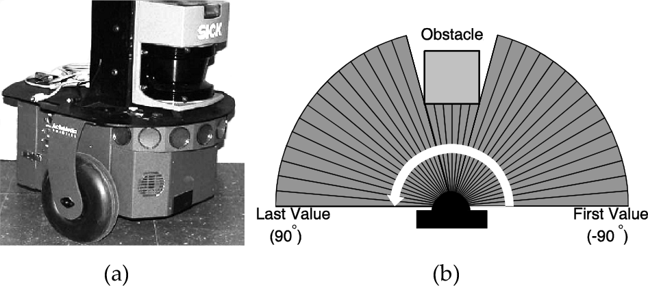
Experimental setup: (a) the mobile robot Pioneer 3- DX with the laser scanner SICK LMS100 onboard; (b) a sketch of the range measurements obtained each sampling time.

Figure 10 illustrates the simulation results for some typical local-minimum environments (Crown-, Zig-Zag and G-shaped obstacles) in which the proposed algorithm has shown to be able to guide the robot to the goal, leaving the obstacles behind. In Figure 10(a) a Zig-Zag obstacle is considered, and the robot path towards the goal is shown. Notice that in this simulation six obstacles are detected, although none of them is detected more than once. In Figures 10(b) and 10(c), in their turn, it is important to highlight the instances in which the mobile robot reaches a point it had already visited (marked with a black circle). To find a new feasible path to the goal, it changes its current orientation to the opposite direction, using the orientation controller of Subsection 2.3, before resuming the navigation. In Figure 10(b), such a manoeuvre occurs when the robot is in the coordinates (2.5m, 2m) and (5.5m, 2m), whereas in Figure 10(c) it occurs when the robot is in the coordinates (1.5m, 0m). As one can notice from the figures, the proposed strategy is effectively able to guide the robot to the goal avoiding such obstacles.

Figure 10.

Distinct obstacle-avoidance simulations.

As for the simulator adopted to generate the results of Figure 10, it is a MATLAB^® code correspondent to the tangential approach, which includes models of the Pioneer 3-DX and its laser rangefinder provided by the manufacturer.

In the sequel, four real experiments are reported and discussed. In the first one the objective is to reach a goal positioned behind a U-shaped obstacle, using the algorithm represented in Figure 8. Figure 11 shows the path the robot followed (part a), the position error, the orientation error and the robot orientation (part b), and the control signals u and ω along the experiment (part c). A description of what happens along the experiment is quite similar to the description of Figure 6, as the experiment aims just to check the effectiveness of the proposed algorithm to overcome U-shaped obstacles. As one can see in the graphics after the robot reaches the real goal (after t = 80 s) effectively α = 0 and ρ < δ. From this moment on, the position error ρ remains unchanged, the linear velocity remains constant at the value u = 0 and ω is varied until the desired final orientation θ_d = 0 is reached, becoming permanently null from this moment on, thus concluding the navigation, as shown in Figures 11(b) and 11(c).

Figure 11.

Avoiding an U-shaped obstacle - a real experiment.

The paths the robot followed during the other three experiments are shown in Figure 12. In such experiments the robot should navigate through a Z-shaped corridor with obstacles in it, and to leave behind an L-shaped and a V-shaped obstacle, respectively. The result is that the tangential escape is effectively able to guide the robot to the goal while avoiding collisions and not getting stuck. A description of the manoeuvres the robot performed along the experiments correspondent to overcome the V and L-shaped obstacles is quite similar to the description associated with Figure 7: the robot starts navigating straightforwardly to the target, as it is well oriented, until entering the obstacle. Then, it manoeuvres to the left and continues navigating. When it “perceives” that both d_min and d_90° are lower than d_obs, it rotates 90° more to the left, and starts following the direction of the obstacle wall. At the end of the obstacle wall, the robot executes the manoeuvre of Figure 7, against the end of the obstacle wall, thus leaving the obstacle behind and taking its way to the target, now in free-space. In terms of the navigation in a Z-corridor with obstacles along it, the robot starts taking a path to go to the target directly, compensating the initial orientation error. Doing that, it naturally avoids the first obstacle, as it navigates towards the left wall of the corridor. Then, it manoeuvres to the right to avoid such wall, and takes a straightforward path to the target again. On going on, the robot detects the right wall of the corridor, and rotates left to avoid it. On doing that, it detects the second obstacle along the corridor and rotates to the right to avoid it, and to the left again, to avoid the end of the corridor wall. After those manoeuvres, it takes a straightforward path to the target, now in the free-space, and continues navigating until reaching the target.

Figure 12.

Other obstacle-avoidance experiments.

Referring to the parameter d_obs involved in the implementation of the tangential escape approach, for the cases of the U-, L- and V-shaped obstacles, its value was 700 mm, while in the case of the Z-shaped corridor its value was 500 mm (due to the small distance between the obstacles along the corridor and the corridor walls). Such values were arbitrarily chosen and could be the same for all simulations and experiments described here.

Therefore, considering the simulations and the experimental results, the conclusion is that the tangential escape is an attractive approach to avoid obstacles when a mobile robot is seeking a goal, because of its low computational cost and its capability of preventing the robot from becoming stuck in local minima. Moreover, the controllers responsible for reducing the distance robot-goal and correcting the final robot orientation - (3) and (6), respectively - are quite easy to design.

Lastly, the figures correspondent to the experiments were built with data collected using the robot odometry (the followed path, the state variables ρ and α, the current orientation ψ and the velocities u and ω effectively developed) and by the laser scanner (the environment layout).

5. Concluding Remarks

A simple and effective approach is proposed here to avoid obstacles when a mobile robot is seeking a goal, which is referred to as the tangential escape. The proposal consists of a supervised nonlinear controller that guides the robot to follow the direction of the tangent to the obstacle border, whenever an obstacle is detected closer to the robot than a specified distance. Through the supervisor, a strategy quite similar to the one adopted by human beings is implemented.

The control system thus implemented is shown to be globally asymptotically stable in the Lyapunov sense, in the absence of obstacles, and able to leave all obstacles behind. Therefore, the proposed approach guarantees that the robot will reach any reachable goal.

Several simulations and experiments, including the hardest obstacles known in the literature, were run using the proposed system, with range measurements provided by a laser scanner. Their results have shown that the proposed controller is effectively able to guide the robot to the goal without colliding with any obstacle or getting stuck in local minima, thus validating the proposal.