Sage Journals: Discover world-class research

Abstract

Simulation is one possibility to gain insight into the behaviour of tracked vehicles on deformable soils. A lot of publications are known on this topic, but most of the simulations described there cannot be run in real-time. The ability to run a simulation in real-time is necessary for driving simulators. This article describes an approach for real-time simulation of a tracked vehicle on deformable soils. The components of the real-time model are as follows: a conventional wheeled vehicle simulated in the Multi Body System software TRUCKSim, a geometric description of landscape, a track model and an interaction model between track and deformable soils based on Bekker theory and Janosi–Hanamoto, on one hand, and between track and vehicle wheels, on the other hand. Landscape, track model, soil model and the interaction are implemented in MATLAB/Simulink. The details of the real-time model are described in this article, and a detailed description of the Multi Body System part is omitted. Simulations with the real-time model are compared to measurements and to a detailed Multi Body System–finite element method model of a tracked vehicle. An application of the real-time model in a driving simulator is presented, in which 13 drivers assess the comfort of a passive and an active suspension of a tracked vehicle.

Keywords

Real-time model driving simulator Multi Body System–finite element method model tracked vehicle

Introduction

Vertical oscillations in tracked vehicles could lead to discomfort, illness or to the increase in injuries in case of transporting injured people. In order to investigate mainly the vertical oscillation, especially with respect to the effect on the human being, driving simulators are a useful option. The main components of a driving simulator are the moveable cabin with viewing and sound system in which the driver or an occupant is sitting, and the real-time computer with the Multi Body System (MBS) software (cf. Figure 1). The motion of the cabin is calculated by the real-time computer and then transferred to the motion system which moves the cabin with the driver. The ability of the real-time computer to calculate the correct movement of the vehicle instantaneously is essential for driving simulation. To do this, special dynamic software is necessary. There are some special commercial MBS software packages available, but the combination of MBS, tracked vehicle, deformable soil and rough uneven terrain is not considered therein.

Figure 1.

Main components of a driving simulator.

In this article, a real-time model consisting of an MBS part for the vehicle (sprung mass, wheels, torsion bar suspension, dampers or actuators) without the track and a MATLAB/Simulink part for the track, the deformable soil, the rough terrain and the interaction between the vehicle, the soil and the track is used in a real-time computer of a driving simulator to compare a passive with an active suspension system of a tracked vehicle. In the literature, a real-time model taking into account the detailed interaction between the track and the wheels of the vehicle, on one hand, and the interaction between the track and deformable soils and the rough terrain, on the other hand, which serves as a model in a driving simulator is not described.

The interaction between vehicles and deformable soils is described in Bekker,^1,2 Wong,³ Garber and Wong,^4,5 Park et al.,⁶ Rubinstein and Hitron⁷ and Yamakawa and Watanabe;⁸ the particular interaction between tracked vehicles and deformable soils is analysed in Garber and Wong,⁴ where an analytical solution is given; MBS models are described in Rubinstein and Hitron,⁷ Yamakawa and Watanabe,⁸ Ma and Perkins,⁹ Wu et al.,¹⁰ Agapov et al.,¹¹ Jothi et al.¹² and Chen et al.¹³ Some aspects, even in new publications, are not considered, for example, multi-pass effects. In Ma and Perkins,⁹ a detailed model of the terrain–track–wheel contact is given; the track is described by finite elements. The deformable soil is described by pressure–sinkage relationship of Bekker¹ and Contreras et al.,¹⁴ and the tangential stresses are calculated using Jonosi–Hanamoto’s law.^14,15 The model is applied to a pair of wheels and to three wheels, each on different soils. Driving of a whole tracked vehicle and multi-pass effects are not considered. The model used¹⁰ is an MBS model additional with the same equations for the description of the soil used in Ma and Perkins.⁹ The model is established using the commercial software RecurDyn. Since there are a lot of rigid bodies, there is no simple way to use the model in real-time for driving simulators. Furthermore, a detailed consideration of the interaction between the track plates and the soil is not possible, because the simple soil models of Bekker and Janosi–Hanamoto are used which do not admit the description of the interaction between complex geometry and the soil, whereas the interaction between complex track geometry and rigid terrain is possible. Furthermore, the laws of Bekker and Janosi–Hanamoto are not able to describe three-axial stress distribution in the soil. For calculation of three-axial stress distribution in the soil, finite element techniques can be used, in combination with an appropriate constitutive law, for example, Drucker–Prager cap.¹⁴ Real-time models for use in driving simulators are seldom described in the publications, merely in Agapov et al.¹¹ a simple real-time approach is described, where the contact forces between the track and terrain depend on the penetration of the nominal track into the terrain, but the track is not deformed by these contact forces. Furthermore, the contact forces between the road wheels and the terrain is calculated using a law similar to Hertzian contact. The approach in Agapov et al.¹¹ is not outlined for (deformable) soils. The results of an MBS model which is extended by simple finite element beam elements for the road wheels arms are presented in Jothi et al.¹² The model is set up using the track model of the commercial software ADAMS/ATV, which is capable to describe the interaction between complex geometry of track elements and rigid terrain; the interaction with soft soils using Bekker’s approach^1,14 is possible, but not used in Jothi et al.¹² Adaptive or active suspensions of tracked vehicle are described in Chen et al.¹³ and Illg et al.,¹⁶ respectively. In Chen et al.,¹³ the commercial software RecurDyn is used (see above). The track model in Illg et al.¹⁶ is simplified and did not take into account the deformation of the track between the road wheels when passing small obstacles. This publication¹⁶ serves merely for a reference of the active suspension which is used in the real-time model for investigation comfort in a driving simulator in the last but one section of this article.

In the real-time approach presented here, the ordinary differential equation (ODE) of the catenary as suggested by Garber and Wong⁴ is used in a discrete form for the description of the geometry of the track between the two road wheels. The pressure–sinkage equation of Bekker^1,14 is used for the pressure distribution, and shear stress is calculated using the approach of Janosi and Hanamoto.^14,15 Thus, the same simple approach as in Ma and Perkins⁹ or Jothi et al.¹² is used.

The elevation profile of the terrain and the soil properties, that is, mainly the Bekker values and the values for shear stress calculation,¹⁵ are stored in so-called lookup tables in MATLAB/Simulink. Therefore, arbitrary functions of the elevation and the soil parameters can be used in the calculation. It is possible to implement the change in these values due to the passing of a vehicle or a road wheel in order to take multi-pass effects into account. Elastic spring back of the soil after its plastic deformation is not taken into account. In a dynamic validation experiment, velocities and angles are compared. In this experiment, the tracked vehicle was driven on a rigid street with obstacles. This experiment was modelled in an MBS–finite element method (FEM) model, too. The aim of this model is to verify correct behaviour of the real-time model, because the comparison between the experiment and model is difficult.

Coupled MBS–FEM model

In order to compare the results of the real-time model to the results of a tracked vehicle driving on deformable soils, a detailed model was created (cf. Figure 2). This model serves only as reference in the development process of the real-time model. The main components of this model are as follows: the body of the tank (rigid body), torsion bar suspension for the road wheels, road wheels, driving sprockets, return rollers, dampers, track tensioner and the tracks, consisting of 60 rigid bodies on both sides. The track is a link track or a segmented metal track with short track pitch (cf. Wong¹⁷).

Figure 2.

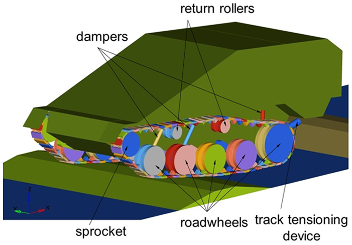
Detailed MBS–FEM model of the tracked vehicle.

The main (rigid) body has 6 degrees of freedom. The inertia properties (mass, centre of gravity, moments of inertia) are the same as in the real-time model and similar to the real vehicle. The parameters of the models are (both FEM–MBS and real-time model; ratios containing the track pitch are not applicable for the real-time model) as follows: the mass is 4.2 t, the average pressure between the track and the soil is 41.9 kN/m², the ratio of small road wheel diameter $D_{w}$ to track pitch $d_{t}$ is $D_{w} / d_{t} = 3.4$ (cf. Figure 3(a)) and the ratio of the small road wheel diameter $D_{w}$ to the track plate length $d_{p}$ (in longitudinal direction) is $D_{w} / d_{p} = 4.7$ . The ratio of the distance of the road wheels $d_{w}$ to track pitch $d_{t}$ is $d_{w} / d_{t} = 4.8$ , which means that nearly five track plates are between the two road wheels, and this results in approximately four links between the two road wheels (the latter number is important for discretization of the catenary in the real-time model).

Figure 3.

(a) Dimensions of the chassis and (b) simplified geometry of the driving sprockets.

The two driving sprockets at the left front and right front of the vehicle have 1 rotational degree of freedom with respect to the main body. The ratio of the small road wheel diameter $D_{w}$ to the sprocket diameter $D_{s}$ is $D_{w} / D_{s} = 1.2$ . The angular velocity of the engine and gearbox is applied to the driving sprockets. The engine and gearbox are not implemented in detail in the MBS–FEM model, but the angular velocities of the sprockets are prescribed as function of time.

A driving sprocket is depicted in Figure 3(b). The teeth shown in the picture are necessary for transmission of forces between driving sprocket and track plates; the details of force transmission are explained below.

In contrary to the other ones, the rear road wheels are not attached to the main body by torsion bar suspension; they have 1 rotational degree of freedom with respect to the track tensioner and the track tensioners themselves have 1 translational degree of freedom with respect to the main body. In parallel to the translation joint, the tension springs are acting. These springs are responsible for the tension forces in the tracks.

The remaining eight road wheels are detached to the main body by torsion bar suspension elements. This means that their centres of gravity have 1 degree of freedom by moving on a circle. The circle is determined by the rigid arms at the end of the torsion bars (Figure 4). The corresponding characteristic force–displacement and force–velocity curves are taken from measurements of the components.

Figure 4.

Rigid arms of torsion bar suspension for the road wheels.

The preload torques of the torsion bars are different for the road wheels, that is, the preloads of the first road wheels are higher than the preloads of the second wheels. Despite the degree of freedom of the centres of the road wheels, they have a rotational degree of freedom. The four smaller return rollers have 1 rotational degree of freedom with respect to the main body. Each track is represented by 60 rigid bodies which are connected by four beams (cf. Figure 5).

Figure 5.

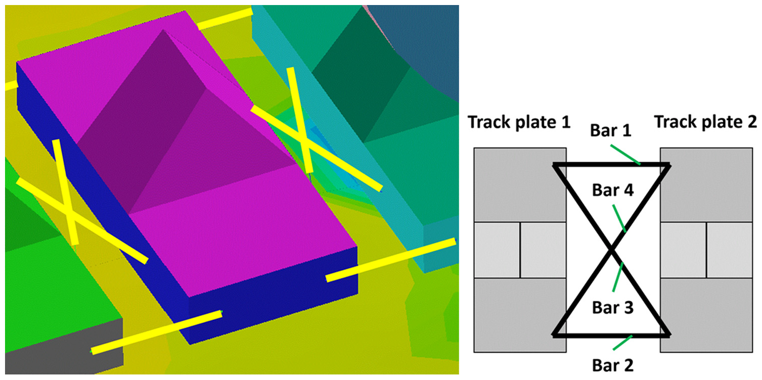
Four very stiff bars as chain links: two longitudinal and two diagonal bars.

The beams are introduced for modelling rotational degree of freedom of the linked plates. This means that the revolute joints including the rubber bushing are approximated. As the beams are very stiff, this approximation ensures the flexibility of the bearings which can be found, for example, in rubber bushings. This way of modelling has the great advantage that no closed chain in the sense of multi-body dynamics has to be introduced. A closed chain would yield a system of differential-algebraic equations which is more expensive to solve than a system of ODEs. The beams are modelled by finite elements; the stiffness is EA/L₁ = 26.1 kN/mm for the longitudinal beams and EA/L₂ = 8.9 kN/mm for the diagonal ones, where L₁ is the length of the shorter beams and L₂ the length of the longer diagonal ones.

The interaction between the tracks on one side and the wheels (driving sprockets, road wheels and return wheels) on the other side is modelled by penalty contact forces. It is obvious that the geometry of the above-mentioned rigid parts (wheels and tracks) is described by segments (triangles and quadrilaterals). The penalty contact algorithm calculates the distances between the nodes of the segments of one part and the segments of the other part. If this distance $Δ s_{c}$ is lower than a so-called contact thickness $h_{c}$ , the penalty forces $F_{c}, F_{c 1}$ , and $F_{c 2}$ are applied to the nodes (cf. Figure 6 for a simple two-dimensional explanation). In this algorithm, the penalty contact force $F_{c}$ is acting on one slave node $K_{1 S}$ , and the forces $F_{c 1}$ and $F_{c 2}$ are acting on the nodes of the master segments $K_{1 M}$ and $K_{2 M}$ , where $F_{c} = F_{c 1} + F_{c 2}$ and where $F_{c} = k_{c} | Δ s_{c} - h_{c} |$ ( $Δ s_{c} < h_{c}$ in Figure 6). For $Δ s_{c} \geq h_{c}$ , the contact forces vanish: $F_{c} = F_{c 1} = F_{c 2} = 0$ . The deformation of the soil is described by an elasto-plastic law similar to Drucker–Prager cap (cf. Contreras et al.¹⁴).

Figure 6.

Penalty contact algorithm in the MBS–FEM model.

One characteristic of this law is that the von Mises yield stress σ_y depends linearly on the hydrostatic pressure p_hyd (cf. Figure 7). The second characteristic is the volumetric plastic behaviour which occurs for hydrostatic stress distribution. Plastic deformation therefore takes place under two conditions: the second invariant of the deviatoric stress tensor exceeds the von Mises yield stress or the hydrostatic pressure exceeds the volumetric pressure curve. Yielding under hydrostatic pressure means a kind of cap in the deviatoric yield curve. This cap is pushed to higher values if the soil is deformed plastically by hydrostatic pressure which means a kind of hardening of the soil. This hardening is necessary for description of multi-pass effects.

Figure 7.

Yield surface of Drucker–Prager cap material law.

Real-time model

The real-time model of the tracked vehicle can be divided into two parts: the MBS part contains the sprung mass (main body of the vehicle), the torsion bar suspension, the dampers (or actuators) and the wheels (driving sprockets and road wheels). Since the track is being supposed to form a straight line between the driving sprockets and the last road wheels, the return rollers can be neglected. The sprung mass has 6 degrees of freedom. With respect to the sprung mass, each sprocket has 1 rotational degree of freedom, each of the eight small road wheels has 2 degrees of freedom (1 rotational with respect to their centre of mass and 1 for the movement of the centre of mass on the circle which is prescribed by the arms of the torsional bar suspensions) and each of the two large road wheels has 2 degrees of freedom (1 rotational with respect to their centre of mass and 1 translational for the movement in direction of the track-tensioning device).

This MBS part is a model in TRUCKSim, a commercial MBS software with the ability of real-time simulation, and the MBS part has the same degrees of freedom as the corresponding part of the MBS–FEM model.

The second part contains the track, the deformable soil and the rough terrain. This part is implemented in MATLAB/Simulink. The interaction between both parts is shown in Figure 8. TRUCKSim and MATLAB/Simulink can be coupled, and a real-time executable programme is built by TRUCKSim, which contains TRUCKSim parts (MBS, powertrain) and MATLAB/Simulink parts (track, soil, terrain and the interaction model). This real-time executable is sent to the real-time computer which controls the driving simulator.

Figure 8.

Interaction of the MBS part (TRUCKSim) and the track with deformable soil.

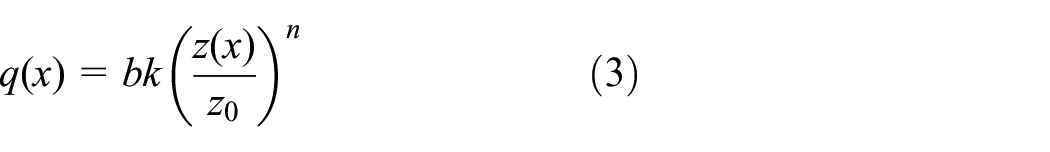
The positions of the wheels are the output values of TRUCKSim and the input values for Simulink. In Simulink, the intersections between the polygons, which connect the vertices of the wheels, and the elevation of the terrain are calculated (first step in Figure 8). These intersections together with the Bekker values and the pressure–sinkage law of Bekker

p = (\frac{k_{c}}{b} + k_{φ}) {(\frac{z}{z_{0}})}^{n}

(1)

yield the pressure distribution under the track (Step 2). Because of the power law with the non-integer power n, we prefer the notation of the law without dimension in (z/z₀)ⁿ. Using the dimensionless equation (1) allows to use SI units for the constants $k_{c}$ and $k_{φ}$ ; furthermore, we avoid units in the constants such as, for example, the square root of a length $\sqrt{10} cm$ . Using the dimensionless equation (1), it is important that the constants depend on the choice of $z_{0}$ .

Resulting from the pressure calculated in the second step, the geometry of the track will follow a catenary line, which is described by the ODE

z ″ (x) = \frac{q (x)}{F_{T}}

(2)

where q is the force distribution (i.e. force per length), $F_{T}$ is the tension force and $z ″ = d^{2} z / d x^{2}$ . The differential equation of the catenary describes a chain or cable without bending moments, for example, in gravitational field. It can be used, too, to describe approximately a chain, as it is done here, which is loaded by a line load. The ODE is an approximation; as the chain links have finite length in reality, the ODE holds for chain links with infinitely small lengths. In the specific case investigated in this article, an interaction occurs between the tension force and the line load, whereas the line load in turn depends on the solution of ODE (2) and the profile of the uneven soil. This interdependency (cf. Figure 8) demands a numerical solution procedure of equation (2); a closed solution does not exist because of the nonlinearities of equation (1), which enter in the line load (the solution of equation (2), the positions of the road wheels, the position of the centre of mass of the whole vehicle and its pitch and roll angles and the profile of the uneven soil determine the local sinkage which enters in equation (1)). Using the catenary differential equation, we neglect torques, for example, from coulomb friction in the chain links, because the load from the weight of the whole vehicle and the forces from propulsion and tension are generally higher than these torques in chain links; therefore the neglection seems to be reasonable. The catenary is approximately calculated by assuming that the ends of the catenary are the vertices of the wheels and the continuously varying pressure distribution is substituted by discrete forces (Step 3).

In the fourth step, the resulting forces as a result of sinkage and the catenary are reimported to TRUCKSim. The starting point of the calculation of the catenary line is the position of the wheel of one side. The vertices of the wheels are connected by straight lines. This auxiliary polygon of vertices is necessary for calculating the sinkage distribution of the track. The polygon is extended in the lateral vehicle direction (widths of the tracks are b) in order to have a contact surface which represents the contact area of the track. This contact surface is intersected with the rough surface of the terrain (or rigid pavement). The depth of the intersection gives with

q (x) = bk {(\frac{z (x)}{z_{0}})}^{n}

(3)

the force distribution.

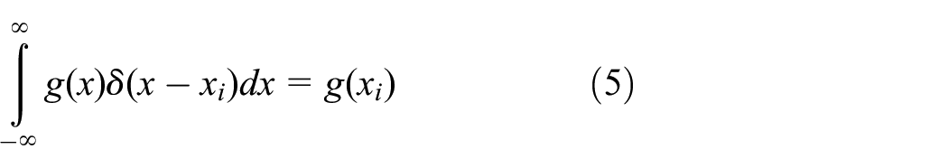
One possible way to continue would be to integrate the differential equation of the catenary line. One goal of the model is the application in real-time; therefore, the pressure distribution of every straight line between the two road wheels of the auxiliary polygon is discretized in six force components $F_{0}, \dots, F_{5}$ , which are entered into the differential equation of the catenary

F_{T} z ″ (x) = \sum_{i = 0}^{5} F_{i} δ (x - x_{i})

(4)

Here, the coordinates x_i = iL/5, $i = 0, \dots, 5$ are the equidistant distributed acting points of the forces and δ is the Dirac’s delta distribution with the known characteristic

\int_{- \infty}^{\infty} g (x) δ (x - x_{i}) dx = g (x_{i})

(5)

and ( $i = 1, \dots, 4$ )

F_{i} = \int_{iL / 5 - L / 10}^{iL / 5 + L / 10} p (ξ) d ξ

(6)

F_{0} = \int_{0}^{L / 10} p (ξ) d ξ

(7)

F_{5} = \int_{L - L / 10}^{L} p (ξ) d ξ

(8)

Integrating equation (4) twice results in the catenary line between the two wheels which is a piecewise linear function

z (x) = \frac{1}{F_{T}} \sum_{i = 0}^{5} F_{i} {〈 x - x_{i} 〉}^{1} + C_{0} + C_{1} x

(9)

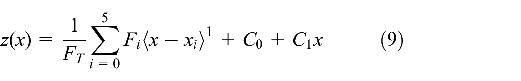
where ${〈 x - x_{i} 〉}^{1}$ is the linear truncated power function defined by

{〈 x - x_{i} 〉}^{1} = {\begin{matrix} x - x_{i} \land x > x_{i} \\ 0 \land x \leq x_{i} \end{matrix}

(10)

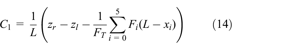
and C₀ and C₁ are the constants of integration which have to be chosen to fulfil the boundary condition of the catenary line, that is

z (x_{0}) = z_{0} = z_{l}

(11)

z (x_{5}) = z_{5} = z_{r}

(12)

where z₁ and z_r are the z-coordinates of the vertices of the left and right wheels, respectively

C_{0} = z_{l}

(13)

C_{1} = \frac{1}{L} (z_{r} - z_{l} - \frac{1}{F_{T}} \sum_{i = 0}^{5} F_{i} (L - x_{i}))

(14)

With this catenary line, the forces acting on the wheels and the length of the catenary line could be calculated. The forces acting on the wheels in the vertical direction from one catenary line between two of them are

{\tilde{F}}_{T 0} = z' (x_{0}) F_{T}

(15)

{\tilde{F}}_{T 5} = z' (x_{5}) F_{T}

(16)

where F_T is the mean track tension force between the two road wheels.

Thus, the forces acting in the vertical direction on the road wheel with the number i are a sum of the forces resulting from the sinkage of the wheel F_Si and the tension forces of the track from the left ${\tilde{F}}_{Til}$ and from the right ${\tilde{F}}_{Tir}$

F_{Vi} = F_{Si} + {\tilde{F}}_{Til} + {\tilde{F}}_{Tir}

(17)

Example

The following example demonstrates that the error due to discrete forces instead of continuous ones is small. Consider the catenary ODE (2) with Bekker’s pressure–sinkage law (3) for the special case n = 1. The forces acting on the left and right ends of the catenary in the vertical direction are $F_{vl} = - 2500 N$ and $F_{vr} = - 2500 N$ , respectively. The tension force is $F_{T} = 15, 000 N$ , the parameter $\tilde{k} = bk / z_{0} = 325 kN / m^{2}$ , the distance between the two wheels $L = 0.6 m$ , $η = \sqrt{\tilde{k} / F_{T}}$ and $x_{m} = L / 2$ . The catenary line is (cf. Garber and Wong⁴)

z (x) = z_{m} \cosh (η (x - x_{m}))

(18)

The equilibrium in z-direction

F_{vl} + F_{vr} = \int_{0}^{L} \tilde{k} z_{m} \cosh (η (x - x_{m})) d x

(19)

yields the maximal deflection $z_{m}$

z_{m} = \frac{(F_{vl} + F_{vr}) η}{\tilde{k} (\sinh (η x_{m}) - \sinh (- η x_{m}))}

(20)

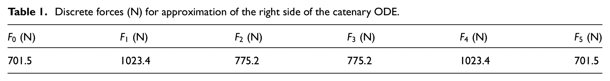
The discrete forces $F_{i}$ are obtained by substituting equation (18) with equation (3) and applying equations (6)–(8) (cf. Table 1). Putting the forces $F_{i}$ in equation (9) and determining the constants $C_{0}$ and $C_{1}$ with $z_{l} = z_{r} = z_{m} \cosh (- η x_{m})$ yields the approximation. The analytical solution and the approximation are depicted in the diagrams of Figure 9. It is obvious that the error between both curves is very small.

Table 1.

Discrete forces (N) for approximation of the right side of the catenary ODE.

$F_{0}$ (N)	$F_{1}$ (N)	$F_{2}$ (N)	$F_{3}$ (N)	$F_{4}$ (N)	$F_{5}$ (N)
701.5	1023.4	775.2	775.2	1023.4	701.5

Figure 9.

Comparison of an analytical solution of the catenary ODE and an approximation in the upper diagram with almost the same scaling of z- and x-axis.

The approximated catenary line yields the forces on the wheels following equation (17) and the length of the line yields the elongation of the track between the two wheels. As the whole track is assumed to be inextensible, the sum of all elongations results in a deflection of the last road wheel with the track tensioner. The length of the catenary line between the two wheels is

ℓ_{c} = \sum_{i = 1}^{5} \sqrt{{(x_{i} - x_{i - 1})}^{2} + {(z_{i} - z_{i - 1})}^{2}}

(21)

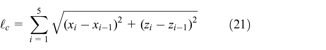
where $(x_{i}, z_{i})$ , $i = 0, \dots, 5$ are the points of the approximation polygon.

Despite the vertical forces, the tangential forces especially traction forces are essential for predicting the vehicle dynamic. The shear stress τ is calculated (cf. Contreras et al.¹⁴) with the following equation

τ = (c + p \tan φ) (1 - e^{- j / K})

(22)

where c is the cohesion, p the vertical pressure, φ the internal friction angle, j the shear displacement and K the deformation modulus of the soil. The model works with arbitrary sets of parameters, and we used parameter sets which are the results of measurements of the IKK (IKK is the former name of IFAS, Institute of Automotive and Powertrain Engineering). The maximum shear stress $τ_{max} = (c + p \tan φ)$ is reached for the infinite values of shear displacements $j \to \infty$ in this model. Thus, the saturation of shear stress at the finite values of shear displacements is not considered here. Of course, this is an approximation of reality, but this modelling yields a stable algorithm because there are no discontinuities or a characteristics with decreasing shear stresses, which often results in numerical unstable algorithms.

The shear displacement $j (t, ζ)$ is calculated at 21 discrete points $ζ_{n}$ : $j_{n} (t) = j (t, ζ_{n})$ , $n = 1, \dots, 21$ . The whole system of equations (MBS part of TRUCKSim and track–soil part of MATLAB/Simulink) is solved by applying a simple time step integration algorithm with a constant time step of $Δ t = 0.001 s$ ( $t_{i} = i Δ t$ ). Thus, the spatial and the time discretization have to be considered in the calculation of $j_{n}$ . Their calculation is illustrated in Figure 10. First, it has to be taken into account that the driving sprocket revolves, and therefore the points $ζ_{n} (t_{i + 1})$ at the next time step $t_{i + 1}$ will not coincide with the points $ζ_{n} (t_{i})$ at time step $t_{i}$ in global coordinate system. Therefore, an approximation for the shear displacement $j_{n} (t_{i + 1})$ is necessary which is using a Taylor expansion (second part in Figure 10)

j (t, ζ - Δ ζ) = j (t, ζ) - \frac{\partial j}{\partial ζ} (t, ζ) Δ ζ + \dots

(23)

Figure 10.

Calculation of the shear displacement.

In discrete form, equation (23) reads

j_{n} (t_{i + 1}) = j_{n} (t_{i}) - \frac{j_{n} (t_{i}) - j_{n - 1} (t_{i})}{Δ ℓ} r ω (t_{i + 1}) Δ t

(24)

where quadratic and higher order terms in $Δ ζ$ are neglected and $j_{0} = j_{1} = 0$ . In equation (24), no change in the shear displacement is considered, that is, it is assumed that $v = r ω$ , where v is the velocity of the vehicle, $ω$ is the angular velocity of the driving sprocket and r is the radius of the driving sprocket. Considering this additional slip $v \neq r ω$ , equation (24) has to be extended (cf. lower part of Figure 10)

\begin{matrix} j_{n} (t_{i + 1}) = & j_{n} (t_{i}) - \frac{j_{n} (t_{i}) - j_{n - 1} (t_{i})}{Δ ℓ} r ω (t_{i + 1}) Δ t \\ + (r ω (t_{i + 1}) - v (t_{i + 1})) Δ t \end{matrix}

(25)

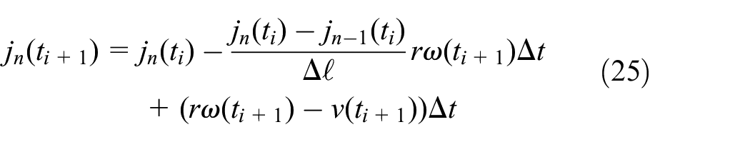
This discrete equation (25) is implemented in the MATLAB/Simulink part of the model as well as the calculation of the tension forces.

Results

In this section, some results of the models are shown. First of all, the models are compared to the experimental results, where the vehicle is driven with nearly constant speed on a rigid street with obstacles. Figure 11 shows the MBS–FEM model with one of these obstacles. In the experimental set up and in the MBS–FEM model, seven and in the real-time model six obstacles are used.

Figure 11.

Vehicle on a rigid street with an obstacle.

One difficulty in comparing the models and the experiment with each other is the translational velocity of the vehicle in the global coordinate system. In the experiment, the velocity fluctuates intensively, cf. Figure 12, and it is increasing.

Figure 12.

Velocity of the vehicle in the experiment, the real-time model and the MBS–FEM model.

The reasons for the fluctuations are the obstacles. As the vehicle has to ‘climb’ them, the velocity decreases; downhill, the velocity increases. In the MBS–FEM model, the angular velocity of the driving sprockets is prescribed, and therefore the fluctuations are smaller than in the experiment. But nevertheless the fluctuations are obvious. Prescribing angular velocities means that the torque of the motor is not limited, and therefore the fluctuations in the MBS–FEM model are smaller than in the experiment.

Another reason for the lack of comparability of the translational velocity is that the velocity in the experiment is measured using the angular velocity of the driving sprockets. In the simulations, the measured velocity is the real velocity of the centre of gravity in the global coordinate system.

Furthermore, the velocity of the real-time is shown in Figure 12. The velocity in the real-time model in this example is controlled by an algorithm, although the velocity is fluctuating. The control driver model of the real-time model in this example (this simulation is done without the driving simulator and without a human being as driver) influences directly the speed of the track by controlling the angular velocity of the sprocket. Thus, the interactions between the vehicle reaction forces, for example, inertial forces, and the engine torque and its characteristic map are not incorporated here for this obstacle test, but these interactions are part of the real-time model used in the investigations with the driving simulator and a human being driver, where a torque–angular velocity-throttle map is implemented. The driver controls the throttle-angle by the gas-pedal. It is not possible to couple a control algorithm with the MBS–FEM model. Therefore, the comparison between MBS–FEM and real-time model is restricted, too.

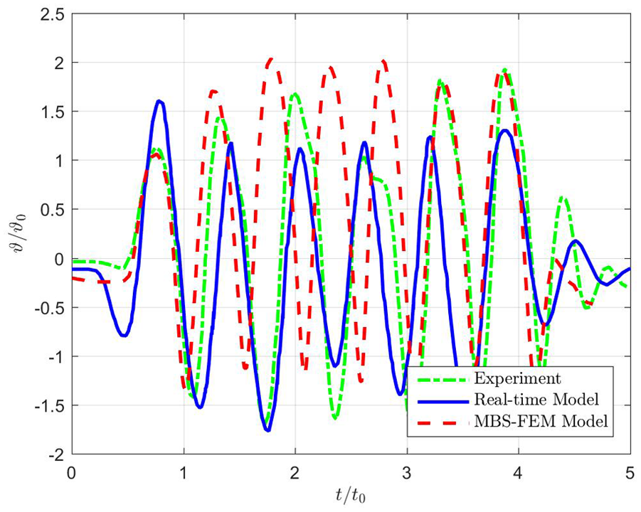
In Figure 13, the pitch angle $θ$ of the vehicle of the experiment, the MBS–FEM model and the real-time model is shown. The similarities are quite good, and the differences are due to the deviation of the velocity (and the different number of obstacles in the real-time simulation).

Figure 13.

Comparison of the pitch angle $θ$ between experiment and real-time model.

In Figure 14, an example of the hydrostatic pressure distribution for a braking manoeuvre for the MBS–FEM model is shown. In Figure 15, the stress component $σ_{zz}$ is shown. The vehicle moves slowly without acceleration. A part of the soil is not shown, that is, a cross section through the soil is visible. The pressure bulb or onion bulb can be recognized clearly.

Figure 14.

Hydrostatic pressure distribution in the MBS–FEM model.

Figure 15.

Pressure bulb $σ_{zz}$ under one track.

Comparison of an active and passive suspension using the driving simulator

The real-time model is applied in control of the driving simulator, cf. Figure 16.

Figure 16.

Hexapod motion system of the driving simulator and viewing system, steering wheel and pedals inside the simulator (right picture).

The driver in the cabin moves on the virtual terrain and its elevation causes vibrations of the cabin. The driving simulator is used to investigate active and passive damping devices. In this investigation, the driver should judge the differences between the passive and active devices. For this purpose, an active suspension (cf. Illg et al.¹⁶) is implemented in MATLAB/Simulink in the real-time model. Then in total, 13 drivers should assess the difference between the active and the passive suspension. The drivers are sitting one after another in the cabin (cf. Figure 16) and driving the real-time model of the tracked vehicle. The driving area is restricted to the orange rectangle of the terrain (cf. Figure 17(a)), where the elevation is shown five times vertical exaggerated. The drivers can switch between the active and passive suspension, and they should grade in the comparison between the active and passive from −3 (passive is clearly better) over 0 (there is no difference between passive and active) to 3 (active is clearly better). The drivers should assess four criteria: the overall comfort, the roll and pitch movements and the vertical oscillations. The results are summarized in Figure 18. The improvement of the pitch is very clear, then the roll is improved and the overall comfort and especially the vertical oscillation are not as good as the first two criteria assessed.

Figure 17.

(a) Terrain for the driving simulator: the area for the investigation is restricted to the orange rectangle and (b) the environment of the investigation with the tracked vehicle.

Figure 18.

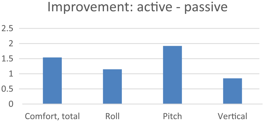
Mean value of the assessments of 13 drivers regarding the active and passive suspension.

Conclusion

A method for creating a real-time model of a tracked vehicle is described. The real-time model consists of an MBS part for the vehicle (sprung mass, wheels, torsion bar suspension, dampers or actuators) without the track and a MATLAB/Simulink part for the track, the deformable soil, the rough terrain and the wheel–track and soil–track interaction. The model can be used in a driving simulator to investigate the interaction between a driver and a tracked vehicle. The track is approximated by a discretization of the catenary ODE. The model is used in a driving simulator to investigate the advantage of an active suspension system for a tracked vehicle. To get an insight into the tracked vehicle driving on deformable soils, in parallel, an MBS–FEM model is used.

Footnotes

Appendix 1

Academic Editor: Hamid Taghavifar

Declaration of conflicting interests

The author(s) declared no potential conflicts of interest with respect to the research, authorship and/or publication of this article.

Funding

The author(s) received no financial support for the research, authorship and/or publication of this article.

References

Bekker

MG.

Theory of land locomotion. Ann Arbor, MI: The University of Michigan Press, 1956.

Bekker

MG.

Introduction to terrain vehicle system. Ann Arbor, MI: The University of Michigan Press, 1969.

Wong

JY.

Terramechanics and off-road vehicles. Amsterdam: Elsevier, 1989.

Garber

Wong

. Prediction of ground pressure distribution under tracked vehicles – part I. An analytical method for predicting ground pressure distribution. J Terramechanics1981; 18: 1–23.

Garber

Wong

. Prediction of ground pressure distribution under tracked vehicles – part II. Effects of design parameters of track-suspension system on ground pressure distribution. J Terramechanics 1981; 18: 71–79.

Park

Chang

Lee

. Prediction of the tractive performance of a flexible tracked vehicle. J Terramechanics 2008; 45: 13–23.

Rubinstein

Hitron

A detailed multi-body model for dynamic simulation of off-road tracked vehicles. J Terramechanics 2004; 41: 163–173.

Yamakawa

Watanabe

A spatial motion analysis model of tracked vehicles with torsion bar type suspension. J Terramechanics 2004; 41: 113–126.

Z-D

Perkins

NC.

A track-wheel-terrain interaction model for dynamic simulation of tracked vehicles. Vehicle Syst Dyn 2002; 37: 401–421.

10.

Z-Y

Gao

Y-D

. Modeling and simulation of tracked vehicle based on Pro/E and RecurDyn. In: Proceedings of the 5th international conference on advanced design and manufacturing engineering (ICADME 2015), Shenzhen, China, 19–20 September 2015. Atlantis Press.

11.

Agapov

Kovalev

Pogorelov

. Real-time model for simulation of tracked vehicles. In: Proceedings of the ECCOMAS thematic conference multibody dynamics 2011 (ed Samin

Fisette

), Brussels, Belgium, 4–7 July 2011.

12.

Jothi

Balamurugan

Malar Mohan

Ride dynamics of a tracked vehicle with a finite element vehicle model. Defence Sci J 2016; 66: 19–25.

13.

Chen

Zhan

Zhou

Modeling and simulation of adaptive surface tracked vehicle based on RecurDyn. Open J Model Simul 2013; 1: 37–41.

14.

Contreras

Foster

. Soil models and vehicle system dynamics. Appl Mech Rev 2013; 65: 040802.

15.

Janosi

Hanamoto

. The analytical determination of drawbar pull as slip for tracked vehicles in deformable soils. In: Proceedings of the 1st international conference on the mechanics of soil-vehicle systems, Torino, 12–16 June 1961. Edizioni Minerva Tecnica.

16.

Illg

Tewes

Jäker

K-P

. Mechatronic design and implementation of an active suspension for an all-terrain tracked vehicle. In: Proceedings of the 9th international symposium on advanced vehicle control (AVEC08), Kobe, Japan, 6–9 October 2008.

17.

Wong

JY.

Theory of ground vehicles. 4th ed.New York: Wiley, 2008.

Real-time model for simulating a tracked vehicle on deformable soils

Abstract

Keywords

Introduction

Coupled MBS–FEM model

Real-time model

Example

Results

Comparison of an active and passive suspension using the driving simulator

Conclusion

Footnotes

Appendix 1

Declaration of conflicting interests

Funding

References