
Abstract
This article proposes a design of a tracking controller for autonomous articulated heavy vehicles (AAHVs) using a nonlinear model predictive control (NLMPC) technique. Despite economic and environmental benefits in freight transportation, articulated heavy vehicles (AHVs) exhibit poor directional performance due to their large sizes, multi-unit vehicle configurations, and high centers of gravity (CGs). AHVs represent a 7.5 times higher risk of traffic accidents than single-unit vehicles (e.g. rigid trucks, cars, etc.) in highway operations. Human driver errors cause about 94% of traffic collisions. However, little attention has been paid to autonomous driving control of AHVs. To increase the safety of AHVs, we design a novel NLMPC-based tracking controller for an AHV, that is, a tractor/semi-trailer combination, and this tracking controller is distinguished from others with the feature of controlling both the lateral and longitudinal motions for both the leading and trailing units. To design the tracking controller, a new prediction AHV model is developed, which represents both the lateral and longitudinal dynamics of the vehicle and captures its rearward amplification feature over high-speed evasive maneuvers. With the proposed tracking controller, the AAHV tracks the predefined reference path and follows a planned forward-speed scheme. Co-simulation demonstrates the effectiveness and robustness of the proposed NLMPC tracking controller.
Keywords
Introduction
Approximately 1.3 million people lose their lives due to road traffic crashes every year. 1 To increase vehicle safety, active vehicle safety systems (AVSSs), for example, vehicle stability control, have been commercialized. 2 These AVSSs can be categorized as “reactive safety systems” (RSSs), devised to react to the current vehicle state. 3 Although RSSs are effective for increasing vehicle safety, they do not consider driver mistakes. The majority (about 94%) of traffic collisions are attributed to human errors. 4 A feasible resolution to the human error problem is autonomous driving, 5 removing human factors from the control loop. The past three decades have witnessed the development of advanced driver assistance systems, for example, lane departure prevention. These systems are known as “predictive safety systems” (PSSs), 3 not only considering current vehicle state, but also predicting vehicle state and hazards in the upcoming time-window. Since the beginning of the 21st century, extensive research has been conducted to explore autonomous vehicle technologies.
To date, most research activities undertaken in autonomous driving have been dedicated to single-unit vehicles. However, little attention has been paid to investigating these PSSs for AHVs.6–8 An AHV is featured with a multi-unit configuration, which is a combination of a towing unit, namely a tractor, and towed unit(s), called trailer(s); each unit is connected to one another at an articulation point(s) by mechanical couplings, for example, fifth wheels. The multi-unit configuration of AHV facilitates freight delivery, improves transportation efficiency, and reduces greenhouse gas emissions.9–11 Despite their economic and environmental benefits, AHVs pose challenges to drivers to control vehicle lateral stability during high-speed lane-change maneuvers due to their multi-unit configurations, long sizes, and high centers of gravity (CGs). 12 AHVs may exhibit exaggerated lateral motion of trailer(s) under high-speed obstacle avoidance maneuvers. Generally, the rearmost trailer shows larger lateral motions than the leading unit; the trailer may be the first unit to roll over; by the time the driver realizes what is happening, it is too late to take a corrective action. 9 A vital indicator for representing the exaggerated lateral motions of the trailer is rearward amplification (RA), defined as the ratio of the maximum lateral acceleration at the rearmost trailer's CG to the maximum lateral acceleration at the CG of the leading unit under evasive maneuvers. 9 AHVs represent a 7.5 times higher risk of traffic accidents than single-unit vehicles in highway operations. 13 It is therefore necessary to put more effort into exploring autonomous driving techniques for AHVs.14,15
Recently, few attempts have been made to develop tracking-control techniques for farm tractor/trailer combinations, 16 heavy-duty mining and construction trucks, 17 and AHVs with automated reverse parking. 18 A path-planning scheme was proposed for tractor/semi-trailer combinations operating in urban environments. 19 These studies share one common feature that they focused on low-speed trajectory-tracking and/or motion-planning based on kinematic control, while ignoring the high-speed RA dynamics and the unstable motion modes of rollover, jackknifing, and trailer sway.
Few scholars tackled the issues of local motion planning and tracking control for autonomous articulated heavy vehicles (AAHVs) in high-speed operations. A path-planning method for single and double lane-change maneuvers at constant speed was proposed.
20
A forward-speed-planning scheme was developed.
21
A robust linear quadratic regulator and a
In the aforementioned past studies on autonomous driving control for AAHVs, the respective local motion-planning and tracking-control designs were based on the output and input variables of the leading vehicle unit alone, while the output variables of the trailing vehicle unit(s) were ignored.22,23 The above design consideration may be attributed to the fact that the actuators for steering and longitudinal accelerating/decelerating are equipped on the leading vehicle unit. However, this design scheme may underestimate the effect of RA dynamics on AHVs. Most of the above trajectory-tracking controllers for AAHVs were essentially path-tracking controllers due to the fact that over curved road negotiations and lane-change maneuvers, vehicle forward speed was assumed to be constant.6–8,22 In reality, the forward speed of an AHV may vary, for example, under an overtaking maneuver in highway operations; under high-speed evasive maneuvers with variable vehicle forward speed, the longitudinal and lateral dynamics of AHVs are interrelated.
This paper is intended to address the aforementioned issues by designing a novel tracking controller for AAHVs. The original contributions of the tracking-controller design for AAHVs lie in (1) both the leading and trailing vehicle units’ lateral and longitudinal motions are controlled considering the output variables of both units in order to improve path-following performance; (2) over high-speed evasive maneuvers, the RA dynamics is emphasized in order to ensure lateral stability; (3) the tracking-controller design fully considers the inherent coupling of longitudinal and lateral dynamics of AHVs over highway evasive maneuvers. To design the PSS-oriented tracking controller for AAHVs, efforts have been made to (i) develop a new prediction vehicle model, which is simple and computationally efficient, yet dependable in capturing the RA dynamics of the AHV with the configuration of tractor/semi-trailer; (ii) develop an effective kinematic model to co-relate the prediction vehicle model with the predefined reference path; and (iii) design novel a model-based predictive control algorithm.
For the proposed controller design, a 7 degrees of freedom (DOF) nonlinear multi-body vehicle model is developed to represent the lateral and longitudinal dynamics of the tractor/semi-trailer combination. The 7-DOF model is used as the prediction vehicle model for the tracking-controller design. Given the 7-DOF nonlinear tractor/semi-trailer model, in the proposed tracking-controller design, the vehicle's forward speed may be treated as a state variable. Thus, the resulting tracking controller is able to handle the operating scenarios while the AAHV negotiates curved paths and conducts evasive maneuvers with variable forward speeds. To co-relate the prediction vehicle model with the target path during the path-following process, a novel kinematic model is developed. To mimic the vehicle plant, a 3-dimensional (3-D) nonlinear vehicle model is generated using a multi-body vehicle dynamics software package, for example, TruckSim. 24
Among various tracking-control techniques, MPC has gained significant popularity due to its ability to handle state and control constraints, thereby permitting tracking-control to operate at the limits of attainable performance. 25 An MPC-based tracking-controller design is generally formulated as an online real-time quadratic optimization problem, in which the current control action is obtained by solving a finite horizon open-loop optimal control problem. The key of MPC is “prediction,” that is, predicting the future evolution of the system and the future action effects over a finite time horizon. Based on the prediction, MPC determines the control actions while minimizing predicted errors subject to operating constraints at each sampling time. 26 In this study, we adopt a nonlinear model predictive control (NLMPC) technique for the tracking controller design. To demonstrate the effectiveness and robustness of the NLMPC-based tracking controller, co-simulations are conducted in an environment, in which the NLMPC controller designed using MatLab/SimuLink is integrated with the virtual tractor/semi-trailer developed in TruckSim.
To design a successful NLMPC-based tracking controller for the AAHV, selecting or developing an effective prediction vehicle model is crucial. This prediction vehicle model is utilized to predict the future states of the tractor/semi-trailer in a finite time horizon; the model should capture the most important dynamic characteristics of the vehicle under the operating maneuvers of interest; moreover, the model needs to be simple, yet computationally efficient since it is included in the NLMPC optimization problem, in which the time to execute the online optimization should be less than the sampling time of the autonomous driving system. Obviously, selecting or developing a vehicle model to satisfy the aforementioned design criteria is challenging. The tractor/semi-trailer model generated in TruckSim is a three-dimensional (3D_ nonlinear model with 33-DOF. This model is frequently used for high-fidelity numerical or real-time simulations. However, this 3D model with 33-DOF is computationally expensive and not suitable to be the predictive vehicle model for online NLMPC optimizations. A linear 3-DOF yaw-plane model is simple in structure and computationally efficient, and it has been used for the MPC-based tracking controller design for a tractor/semi-trailer. 7 Unfortunately, this 3-DOF model can only imitate the lateral dynamics of the tractor/semi-trailer, and it cannot be used for the vehicle's longitudinal dynamic control. A nonlinear 10-DOF yaw-plane model was developed and used for the design of an NLMPC-based tracking controller for controlling both the lateral and longitudinal dynamics of a tractor/semi-trailer. 23 This nonlinear 10-DOF yaw-plane model represents the state-of-the-art prediction model development for NLMPC controller designs for tractor/semi-trailer combinations. However, this model exhibits the following drawbacks: (a) in the tire dynamic modeling, the correlations between lateral and longitudinal tire forces are ignored; (b) in the trajectory-tracking kinematic modeling, the relative errors of the orientation and lateral displacement of the trailer with respect to the target path are neglected; (3) the vehicle forward-speed of interest is around 72 km/h, at which the RA dynamics of the vehicle may not be fully exhibited and evaluated. Built upon the past studies in developing prediction vehicle models for MPC-based tracking-controller designs for tractor/semi-trailers, the nonlinear 7-DOF yaw-plane model is developed in this study.
The rest of the paper is organized as follows. Section 2 “Multi-body vehicle system modeling” introduces the multi-body dynamic models of the tractor/semi-trailer combination. Section “Trajectory tracking of tractor/semi-trailer combination” briefly introduces the concept of local motion planning, defines the reference motion trajectory, and establishes the kinematics for tractor/semi-trailer path-tracking. Section “Design of NLMPC-based tracking-controller” describes the design of the NLMPC-based tracking-controller. The selected simulation results will be analyzed and discussed in the “Results and discussion” section. Finally, the “Conclusions” section concludes.
Multi-body vehicle system modeling
To design the NLMPC-based tracking controller, a 7-DOF nonlinear tractor/semi-trailer model is developed as the prediction model, and the corresponding 3D TruckSim model is generated to mimic the vehicle plant. The prediction model and the virtual vehicle plant play different roles in the NLMPC-based tracking-controller design. As shown in Figure 7, the prediction vehicle model and the MPC optimizer are two essential elements of the NLMPC controller, which is formulated as an online real-time quadratic optimization problem. The design requirements for the prediction vehicle model are: (a) in terms of computational efficiency, the simulation using the model should be faster than real-time; (b) the model needs to characterize the RA dynamics and represent the inherent coupling of the longitudinal and lateral dynamics of the AHV over evasive maneuvers in highway operations. To accommodate these requirements, the 7-DOF nonlinear tractor/semi-trailer model is developed. To mimic the actual tractor/semi-trailer combination, a high-fidelity model is required and the 3D nonlinear model with 33-DOF is generated using TruckSim software. These two vehicle models are described in the following subsections.
7-DOF nonlinear tractor/semi-trailer model
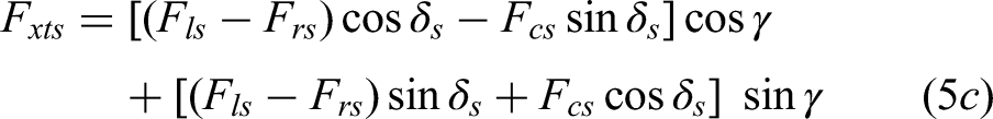
Figure 1 shows the 7-DOF nonlinear model for representing the dynamics of the tractor/semi-trailer combination. As seen in the figure, the tractor/semi-trailer combination is telescoped laterally, and each axle set of the tractor and trailer is represented by a single wheel. Three coordinate systems are introduced: (a) the inertial coordinate system,
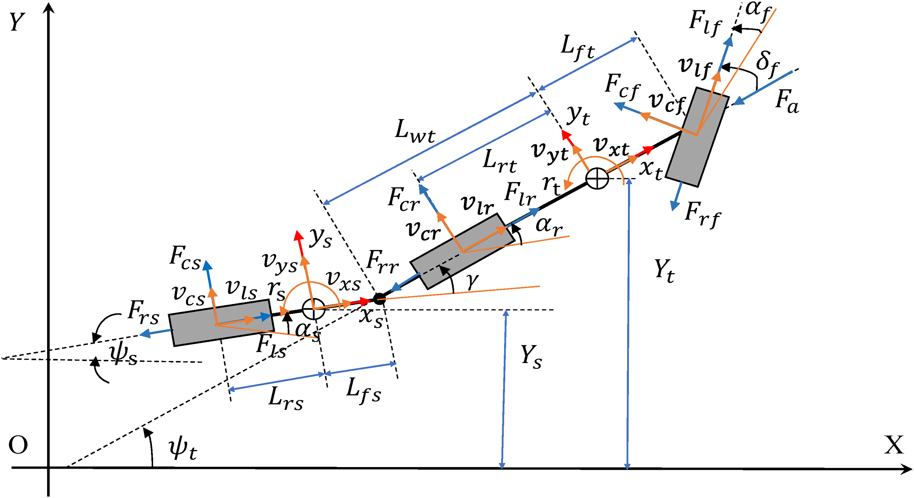
Seven degrees of freedom (7-DOF) nonlinear tractor/semi-trailer model.
In the 7-DOF nonlinear single-track model, seven motions are considered, including tractor lateral motion, tractor longitudinal motion, tractor yaw motion, trailer yaw motion, as well as spinning motion of tractor front wheel, tractor rear wheel, and trailer wheel. The following assumptions are made: (a) the tractor and trailer are treated as two rigid bodies, which are connected by a revolute joint; (b) for the rigid bodies of a tractor and trailer, vertical, pitch, and roll motions are ignored; and (c) the vehicle units’ masses are lumped at the respective CGs with corresponding mass moments of inertia around the vertical axes of their body-fixed coordinate systems.
Rigid-body dynamics
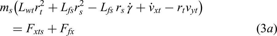
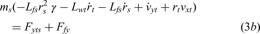
According to the above rigid-body assumption and other simplifications, the equations of motion of the tractor/semi-trailer combination are derived following Newton's law of dynamics. The governing equations of the longitudinal, lateral, and yaw motions of the tractor expressed in the tractor body-fixed coordinate system are given as


The governing equations of the longitudinal, lateral, and yaw motions of the trailer expressed in the tractor body-fixed coordinate system are expressed as

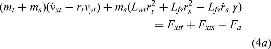
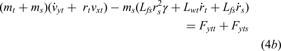
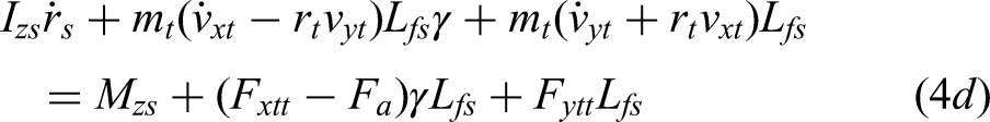
Combining equations (1) and (3) and eliminating the coupling forces at the fifth wheel leads to the following governing equations of motion of the tractor/semi-trailer combination expressed in the tractor body-fixed coordinate system as


Tire and wheel dynamics
The slip angles for tractor and trailer tires can be calculated by

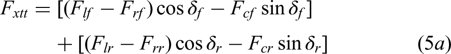
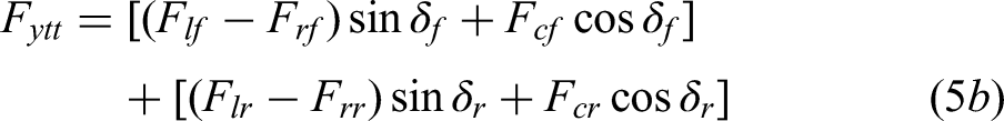
The tire forces are calculated using the Dugoff tire model,27,28 by which, the longitudinal and cornering tire forces, that is,
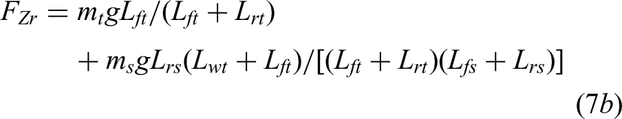


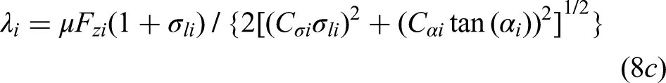
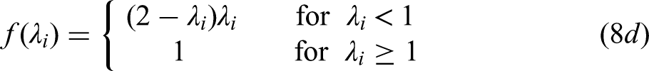

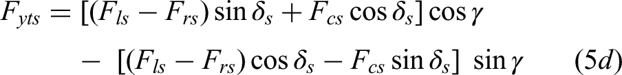
In equation (9), the wheel angular velocities,


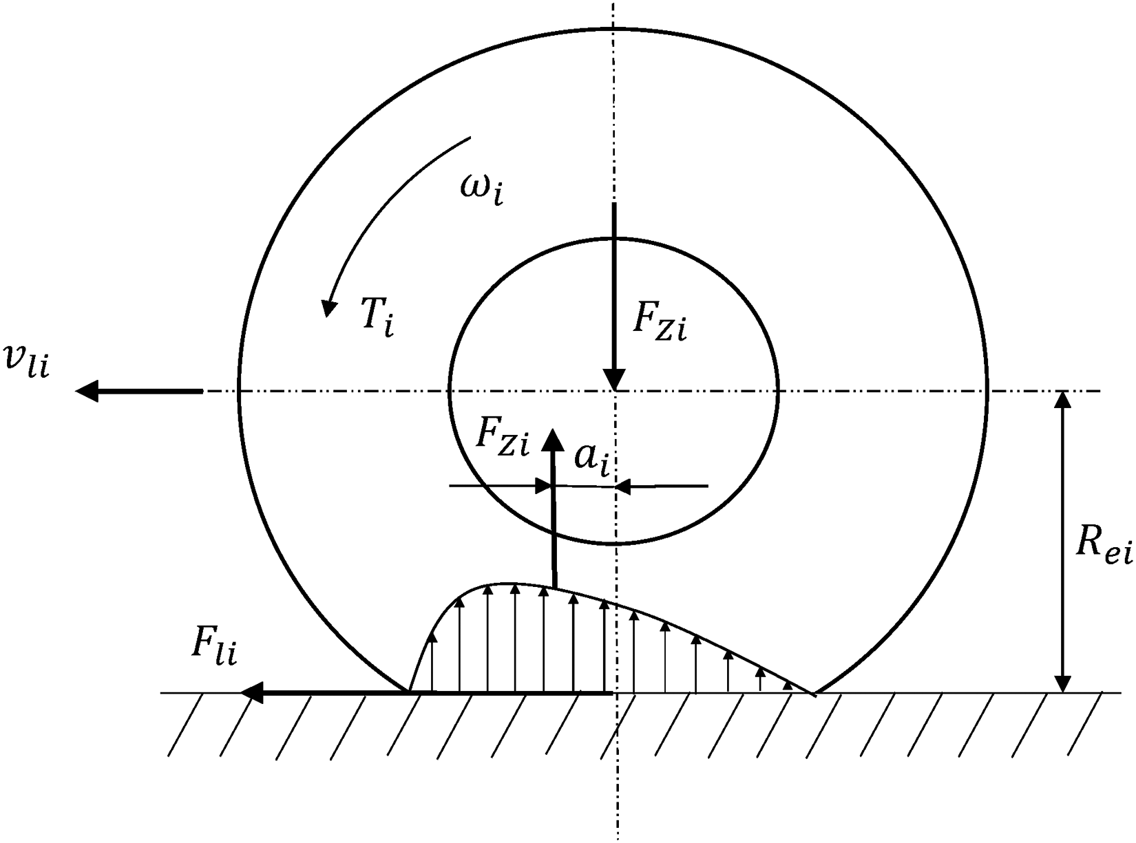
Schematic representation of the wheel dynamics.
Equations (4) and (10a) govern the 7 motions of the tractor/semi-trailer model. The vehicle model can be expressed in a compact form as


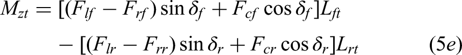
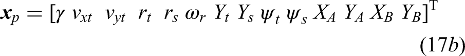
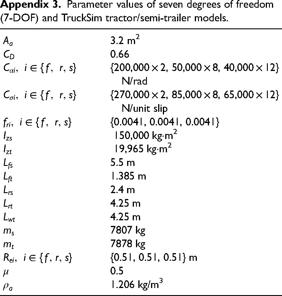
In this study, the 7-DOF tractor/semi-trailer nonlinear model is developed using Matlab/Simulink, and the associated elements/submodels, for example, the wheel model, Dugoff tire model, rigid-body model, etc., are integrated following the structure arrangement shown in Figure 3. The values of the relevant parameters (e.g. geometric and inertial) of the vehicle model are listed in Appendix 3. Given an initial condition and an operating maneuver, the structured simultaneous equations of motion of the vehicle model can be solved, and the resultant state variable vector,
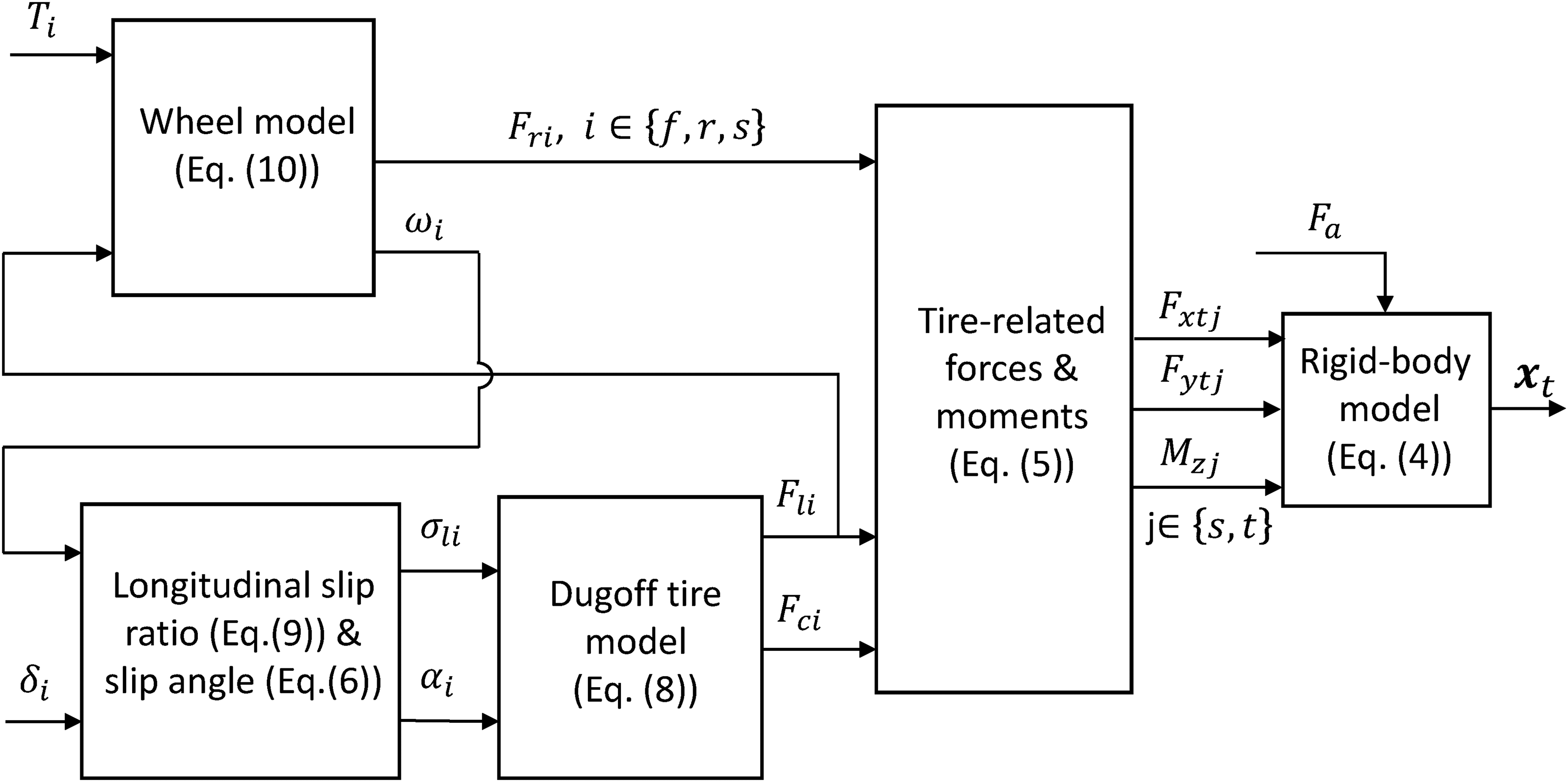
Structure arrangement of the elements/sub-models of the seven-degrees of freedom (7-DOF) nonlinear tractor-semi-trailer model.
It should be mentioned that if the tracking controller (to be designed in the Design of NLMPC-based tracking controller) only controls the lateral dynamics of AHVs at high speeds, the 3-DOF linear yaw-plane model is frequently used.7,8 However, if the tracking controller also needs to control an additional longitudinal motion of the vehicle, built upon the 3-DOF linear yaw-plane model, adding the spinning motion for each of the tractor and trailer wheels and the longitudinal motion of the vehicle leads to the 7-DOF nonlinear tractor/semi-trailer model shown in Figure 3. Given the 7-DOF nonlinear prediction vehicle model, the nonlinear model predictive control technique has to be used.
Trucksim model
The 3D nonlinear tractor/semi-trailer model is generated using TruckSim software, which employs a symbolic multibody program, VehicleSim (VS) Lisp, to derive equations of motion. 24 As shown in Figure 4, the configuration of the tractor/semi-trailer combination is defined as “S_SS + SSS,” where “S” represents a solid axle, an underscore “_” is a separation of axle group, and a “+” a fifth-wheel connecting the two vehicle units. The TruckSim model assumes the nonlinear dynamics of suspension systems, pneumatic tires, and mechanical joints. The 3D vehicle model consists of rigid bodies for representing the sprung masses of the tractor and semi-trailer, as well as six axles. Each rigid body is allowed to move longitudinally, laterally, and vertically, as well as to rotate in roll, pitch, and yaw. The fifth wheel is modeled as a ball joint, about which roll, yaw, and pitch motions are permitted. Each axle is considered a beam, which can roll and bounce with respect to the sprung mass to which it is attached. Each wheel is modeled with a rotating DOF. Using TruckSim software, we thus model the tractor/semi-trailer combination as a 33-DOF nonlinear model.
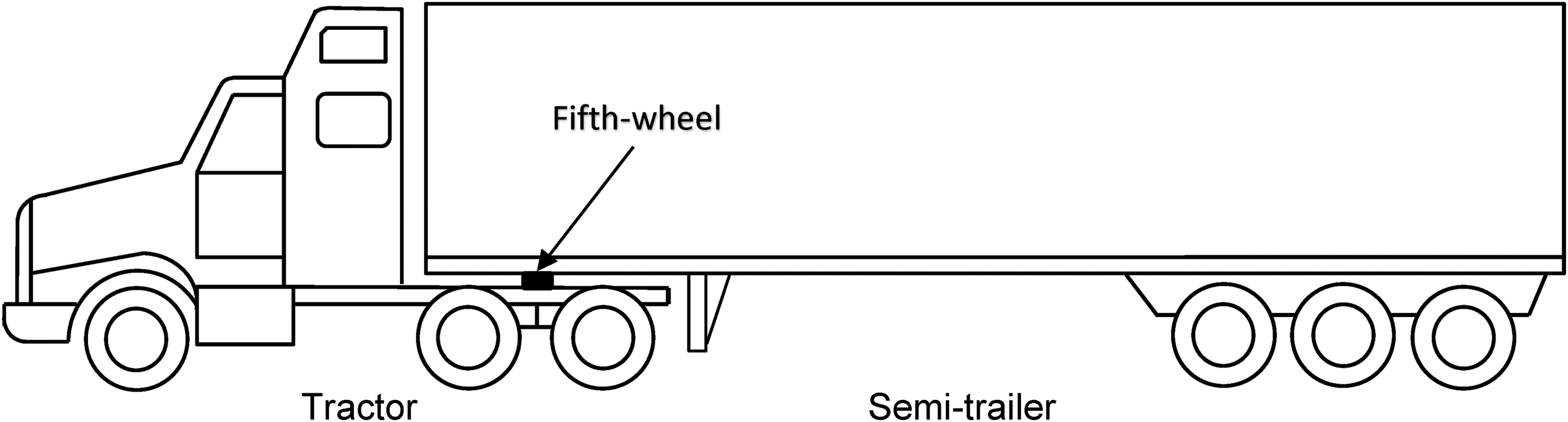
Configuration of the tractor/semi-trailer combination.
In addition, the tractor is modeled with the drive setting of 6 × 4, in which the two rear axles are drive axles. The built-in powertrain model consists of a diesel engine with a power capacity of 330 kW, a mechanical clutch, a gearbox with 18 gear ratios, and a final drive unit with a gear ratio of 4.4.
33
In the built-in braking system model, the control input pressure from the master cylinder is proportioned for each wheel-end brake actuator, and the brake torque is assumed as a nonlinear function of actuator pressure. For the 3D TruckSim model, the forward speed is controlled using the throttle and brake positions, that is,
The TruckSim software was built upon the symbolic multibody program, VS Lisp, for deriving equations of motion for 3D vehicle systems. An input to the VS Lisp describes the 3-D vehicle model structure mostly in geometric terms, for example, sprung mass DOF, point locations, and directions of force vectors. Upon receiving the input, the VS Lisp derives equations of motion in terms of ordinary differential equations and generates a computer source code (C or Fortran) to solve them. The TruckSim software comprises three main components, i.e., VS browser, TruckSim databases, and VS solver. The VS browser serves as a graphical user interface to TruckSim. The browser may also be used for other applications, e.g., incorporating the tracking controller to be devised using Matlab/Simulink into the 3D TrcukSim model via the interface for co-simulation. The VS solver is employed to solve the derived governing equations of motion of the vehicle model and to execute the defined simulations.
Trajectory tracking of tractor/semi-trailer combination
This section introduces the associated concepts of local motion planning, reference trajectory determination, and kinematics for path tracking.
Local motion planning
For an autonomous vehicle, the motion planning and decision module is featured with hierarchically structured sub-modules, which include route planning at the top level, behavioral planning at the middle level, and local motion planning at the bottom level. 34 In the operation of the module, the route planning determines the global route, and the behavioral planner then decides on a local driving task with a motion specification (e.g. turn-left, lane-change, or cruise-in-line). With the directives of the behavioral planner, the local motion-planning sub-module generates the reference trajectory for the tracking controller to track.
The local motion-planning techniques may be categorized into two types 35 : (a) separated approaches, by which spatial maneuver, for example, a single lane-change (SLC) for obstacle avoidance, and temporal maneuver, such as speeding up along the predefined SLC path to overtake a preceding vehicle, are separately planned; (b) integrated methods, with which the spatial and temporal maneuvers are planned simultaneously. The second type shows poor computational efficiency, while the first one significantly improves computational efficiency due to its layered nature. 36
In this study, we adopt separate methods. In the case concerned, a tracking controller is designed for the tractor/semi-trailer combination, and it will be evaluated in an SLC overtaking maneuver in highway operations. Thus, the local motion planning is to determine a collision-free SLC path and to plan a forward-speed scheme over the maneuver.
Reference motion trajectory determination
To evaluate path-following performance and lateral stability of AHVs, a high-speed obstacle avoidance testing procedure is recommended by ISO-14791,
37
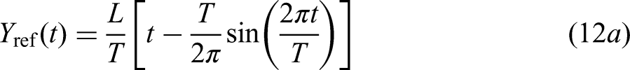
in which the SLC path is prescribed. Over the SLC testing maneuver, the vehicle's forward speed remains constant. To tailor an experiment procedure for the SLC overtaking maneuver in highway operations, a testing course and a speed profile are established on the ISO-14791 recommended procedure.38,39 It is assumed that during the overtaking maneuver, the tractor/semi-trailer travels in the longitudinal direction at a constant acceleration, and the lateral acceleration time history of the tractor is a single-cycle sine wave with a given amplitude and time period. Under highway operations, the geometric path of the overtaking maneuver is defined in the inertial coordinate system and expressed by


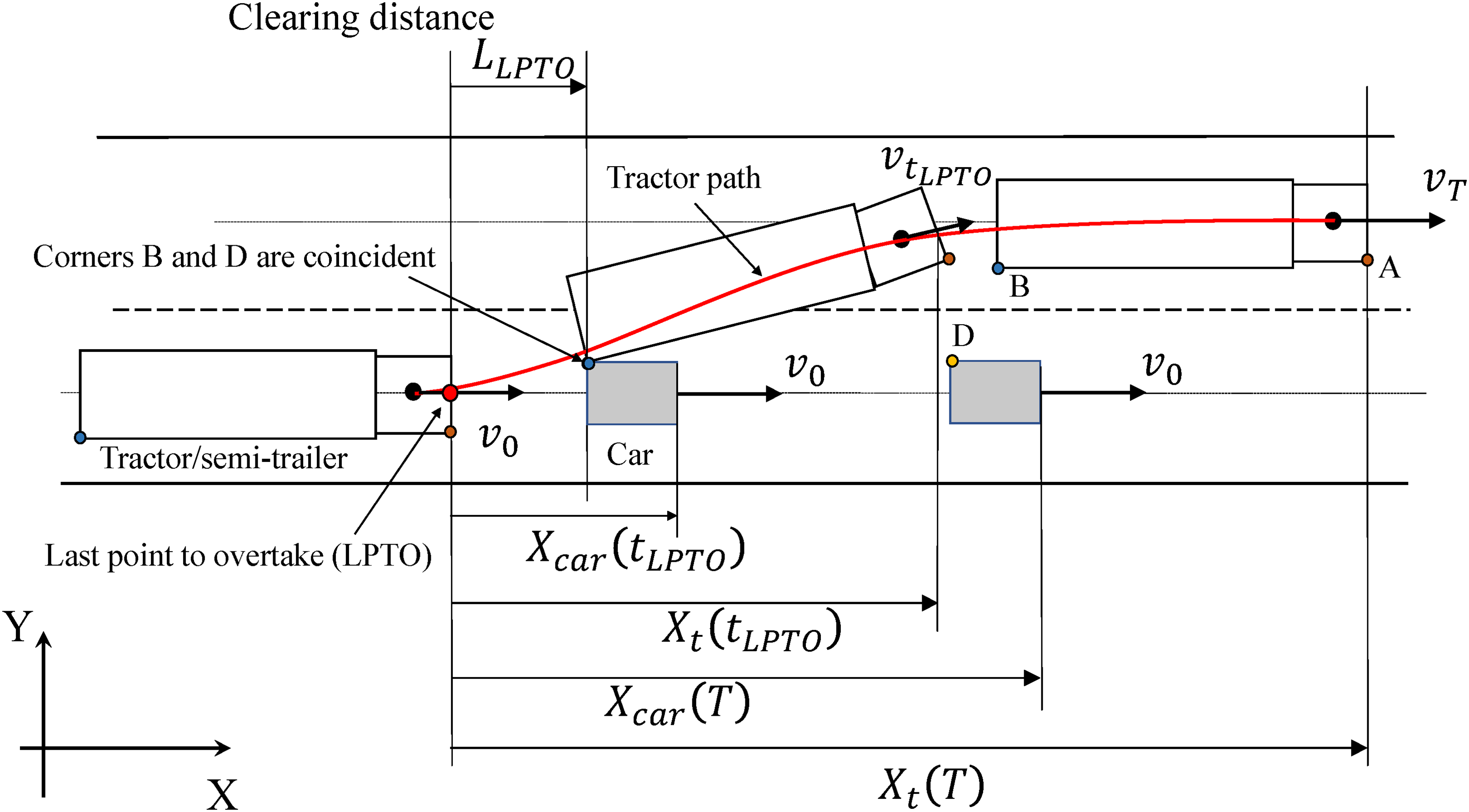
Single lane-change overtaking maneuver.
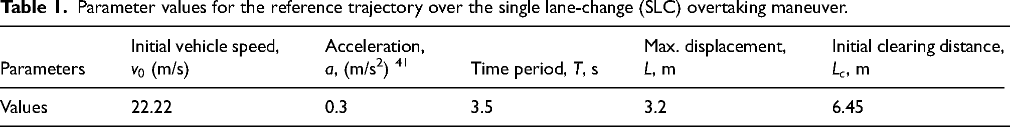
Built upon the numerical simulation using the TruckSim model, the fine-tuned values for the parameters of the reference trajectory for the SLC overtaking maneuver are determined, and they are listed in Table 1. Given the maneuver parameter values, the reference path for the tractor can be specified as shown in Figure 5. It should be mentioned and assumed that prior to the above local motion planning, behavioral planning has already been conducted and predicts the local motion of the preceding car shown in Figure 5. Thus, in the finite future time window, the operation of the obstacle car is predictable. To detect the state of the preceding car, the AAHV may use onboard sensors, for example, RADAR, LIDAR, CAMERAS, etc., and relevant sensor fusion techniques.
Parameter values for the reference trajectory over the single lane-change (SLC) overtaking maneuver.
Kinematics of tractor/semi-trailer path-tracking
Given the prediction vehicle model developed in the 7-DOF nonlinear tractor/semi-trailer model and the reference motion trajectory for the SLC overtaking maneuver determined in the “Reference motion trajectory determination” section, this subsection establishes the kinematics for the AHV tracking the reference path.
Figure 6 shows the geometry representation of the tractor/semi-trailer combination and the target path to be tracked. The target path is defined in the inertial coordinate system. At time t, the coordinates of the tractor and trailer CGs in the inertial coordinate system can be determined by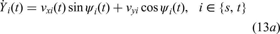


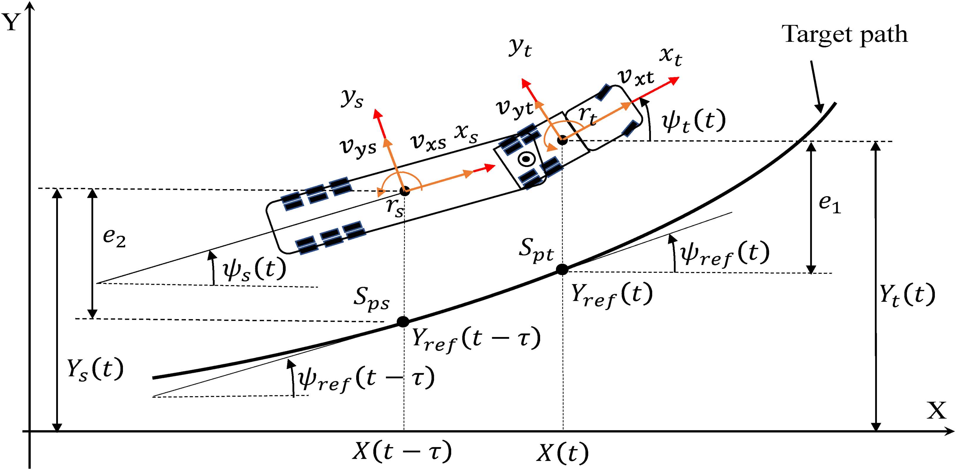
Geometry representation of the tractor/semi-trailer combination and target path.
The horizontal coordinates of the tractor and semi-trailer in the inertial coordinate system are 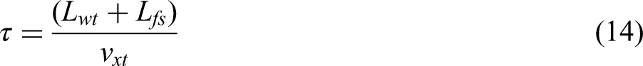
As seen in Figure 6, the cross-track errors of the tractor and semi-trailer can be specified by


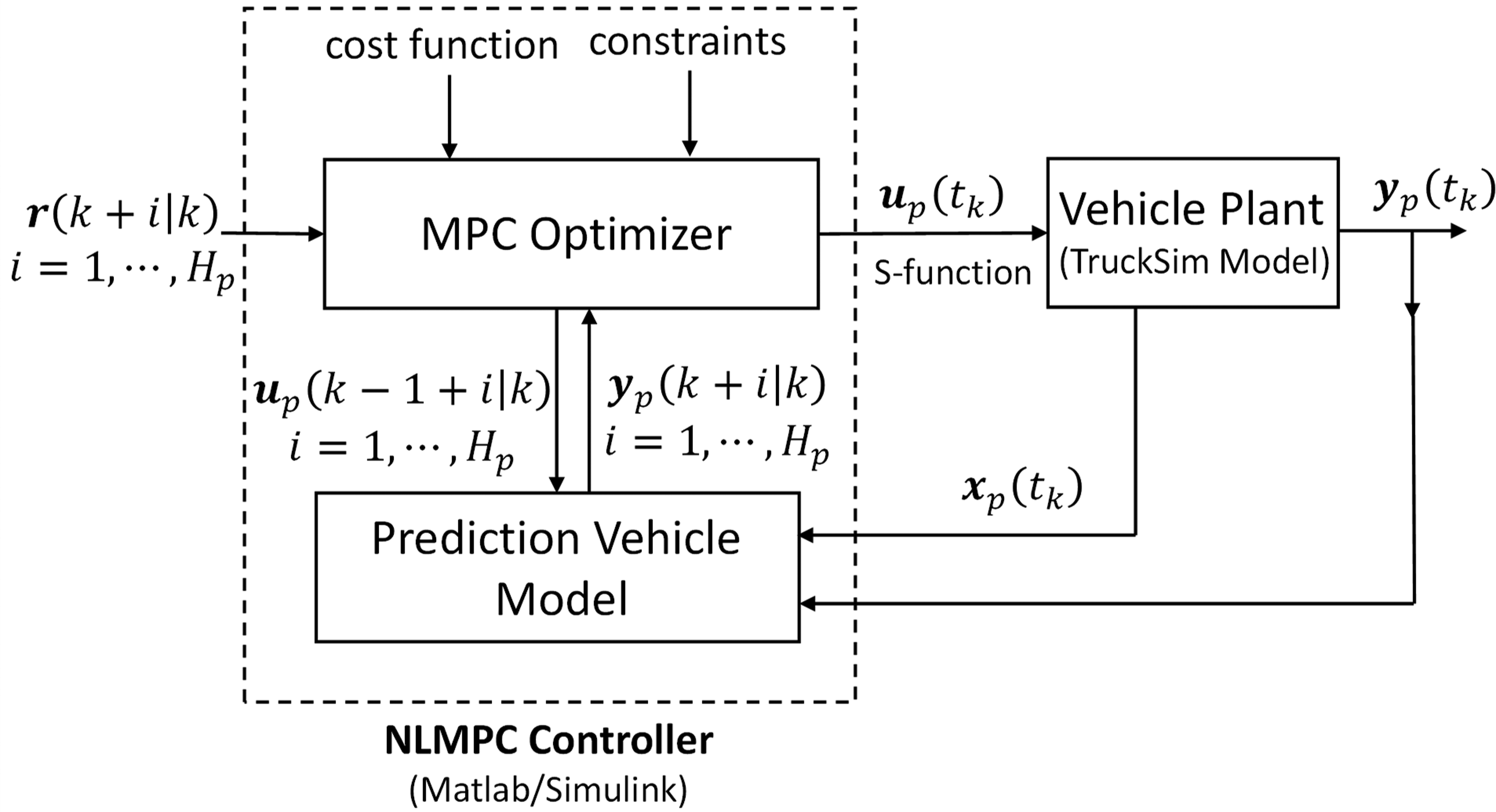
Block diagram describing the interrelations among nonlinear model predictive control (NLMPC) controller and vehicle plant.
It should be mentioned that in the path-tracking kinematic modeling reported in the literature,22,23 the relative errors of the orientation and lateral displacement of the trailer with respect to the target path shown in Figure 6 were not specified.
Design of NLMPC-based tracking controller
This section discretizes the prediction vehicle model represented by equation (17) and specifies output variables. The design of the NLMPC-based tracking controller is then formulated. It should be emphasized that the design objective of the tracking controller is to calculate the tractor front wheel steering angle and the tractor rear wheel driving torque in order to track as closely as possible the reference motion trajectory planned in the “Reference motion trajectory determination” section.
Discretized prediction vehicle model
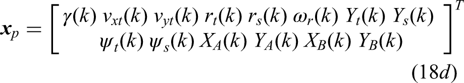
At sampling step k, discretizing the nonlinear prediction vehicle model represented by equation (17) with the forward Euler method leads to


NLMPC controller design
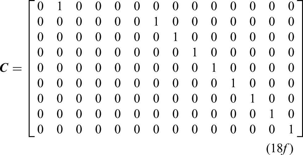
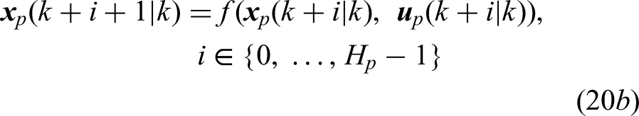
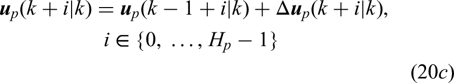
The NLMPC controller consists of two core components: (a) the discretized prediction vehicle model represented by equation (18); and (b) an optimizer with a cost function and a group of constraints. The prediction vehicle model is used to predict the future evolution of the tractor/semi-trailer combination. At a sampling time, beginning with the current state of the virtual vehicle plant, that is, the 3D TruckSim model, an open-loop optimal control problem is solved over a short time window. This online optimization problem minimizes the errors between the predicted outputs and the reference trajectories over a sequence of future control inputs, subject to associated constraints. The resulting optimal control input is applied to the virtual plant, prior to the following sampling interval. At the next time step, a new optimal control problem based on a new set of states of the vehicle system is solved over a shifted time window. This “receding horizon implementation” makes the NLMPC algorithm a feedback controller.
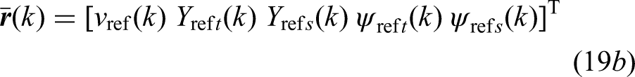
With the vectors of control input, output variable, and reference variable, which are defined by equations (18b), (18g), and (19), respectively, the NLMPC controller design is formulated as a constrained optimization problem with the following cost function subject to the specified constraints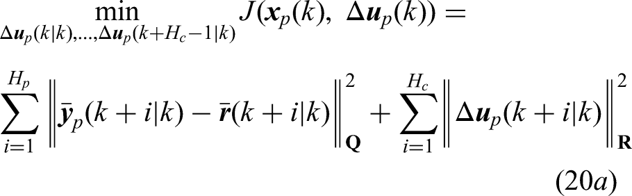


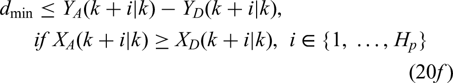
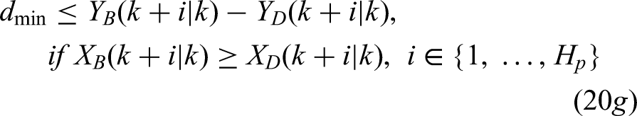
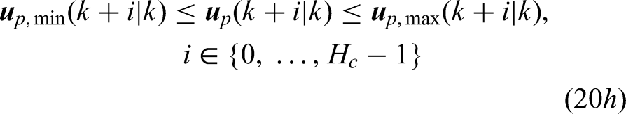
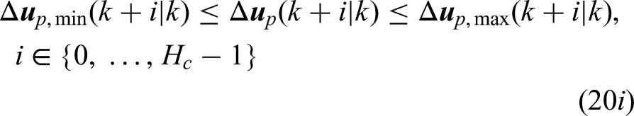

In addition to tracking the reference longitudinal speed
On the right-hand side of equation (20a), the first summand imposes the penalty on trajectory tracking deviation, while the second summand is to prevent large control effort for the automated driving. Solving the optimization problem formulated in (20), we obtain the optimal control input increments evaluated at the sampling step k for the currently observed vehicle state vector 

To summarize the NLMPC controller design, we visualize the interrelations among the MPC optimizer, the prediction vehicle model, and the vehicle plant using the block diagram shown in Figure 7. Note that in the figure, the time instant
Results and discussion
To evaluate the proposed NLMPC tracking controller, co-simulations are conducted for the virtual AAHV to perform the SLC maneuver specified in the “Reference motion trajectory determination” section. For examining the robustness of the tracking controller, co-simulations are also performed under the SLC maneuver with varied trailer payload and under a double lane-change (DLC) maneuver. This section first selects the parameter values of the NLMPC controller, ego vehicle, and traffic environment. The selected parameter values for the NLMPC controller are also justified. The chosen simulation results are then presented.
Selecting parameter values of NLMPC controller, ego vehicle, and environment
As shown in Figure 7, the co-simulation for evaluating the NLMPC controller is directly associated with the reference motion trajectory, the NLMPC controller (consisting of the MPC optimizer and the prediction vehicle model), and the “vehicle plant,” that is, the 3D TruckSim model. The parameter values for the prediction vehicle model and the 3D TruckSim model are provided in Appendices C and D. The reference trajectory is parameterized as a sinusoidal function of time and is determined by the lateral/longitudinal position and longitudinal speed of the AAHV, as well as the forward-speed of the obstacle car at the starting point of the overtaking maneuver. The parameter values for the reference trajectory over the overtaking maneuver are listed in Table 1. The NLMPC controller parameters may be categorized into two groups: (a) tuning parameters and (b) constraint parameters. The following subsections select and justify the values for these NLMPC controller parameters.
Values selection for tuning parameters of NLMPC controller
In MPC controller designs, the tuning parameters generally include42,43: prediction horizon,
Specifying sampling time
In the design of robust tracking controllers using the LQR and
Selecting prediction and control horizons
Reliable guidelines for selecting the tuning parameters of the prediction horizon,
In MPC controller designs for autonomous vehicles, the prediction horizon,
To tune the parameters of
Interestingly, the above-fine-tuned values of Small m means fewer variables to compute in the QP solved at each control interval, which promotes faster computations. If the plant includes delays, m < p is essential. Otherwise, some MV moves might not affect any of the plant outputs before the end of the prediction horizon, leading to a singular QP Hessian matrix. To check for a violation of this condition, use the review command. Small m promotes (but does not guarantee) an internally stable controller.”
Note that in the above-cited tips, m and p denote the control and prediction horizons, that is,
Tuning output and control input variation weight matrices
The selection of the diagonal weight matrices,
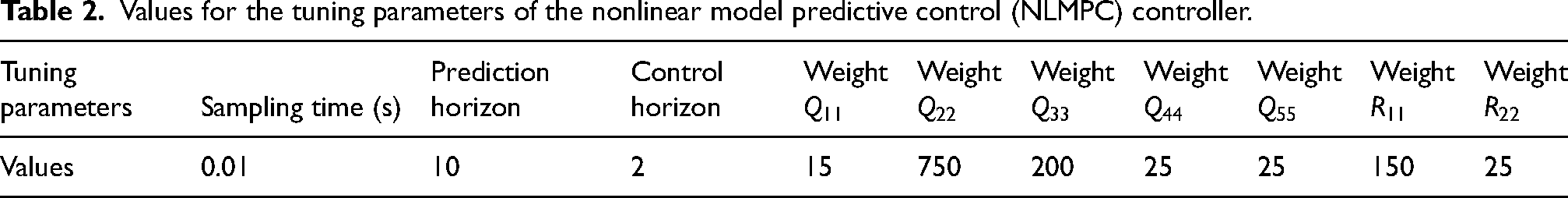
Values for the tuning parameters of the nonlinear model predictive control (NLMPC) controller.
Values selection for constraint parameters of NLMPC controller
In the NLMPC controller design, the constraints specified in (20e) to (20i) reflect the associated vehicle physical limits and design requirements. Considering the longitudinal comfort and time efficiency, we set the forward-speed limits to be
To ensure comfort and stable lateral motions during the overtaking maneuver, we set the tractor front wheel steering angle limits to be 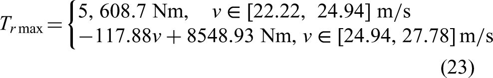
Table 3 summarizes and lists the values of the constraint parameters of the NLMPC controller.
Values of the constraint parameters of the nonlinear model predictive control (NLMPC) controller.

As shown in Figure 7, the NLMPC controller design consists of two essential components, that is, the MPC optimizer and the prediction vehicle model. In turn, the former involves the constrained optimization formulated in (20) and a search algorithm. In this study, the built-in solver in Matlab, that is, sequential quadratic programming (SQP), is used as the search algorithm. The latter is represented by the discretized AHV model expressed in (18). In this nonlinear programming problem, a challenge is confronted: either the nonlinear iteration search is carried out until a predefined convergence criterion is satisfied, thereby possibly leading to considerable feedback delays, or the search is terminated prematurely with only an approximate solution, thus, the prescribed sampling time limit can be met. Given the default SQP search algorithm in Matlab, the efforts for addressing this challenge are summarized as follows:
Developing the “faster than real-time” prediction vehicle model, in which the simple, yet effective powertrain model, as well as the Dugoff tire model, are incorporated. It should be mentioned that the Dugoff tire model is simpler in structure compared to the brush model,
52
moreover, it needs less computational load than the Magic Formula model.
53
As described in equations (7) to (9), the Dugoff tire model is essentially an analytical model, which can be differentiable with respect to the state and control variables, for example, Selecting the effective tuning and constraint parameters for the NLMPC controller. As aforementioned, selecting a small
The impact of taking the above measures is two-fold. First, the computational efficiency of the nonlinear programming problem can be increased, thereby resulting in a more accurate solution. Second, the stability of the NLMPC controller can be enhanced.
Selected simulation results
In the simulation experiments, two trajectory-tracking control schemes are designed. In the first scheme, as shown in Figure 6, for both the leading and trailing vehicle units, trajectory-tracking controls are implemented; while in the second scheme, only tractor trajectory-tracking control is conducted. To examine the robustness of the proposed tracking controller, two case studies are performed. In the first case study, considering vehicle system parameter uncertainties, an additional payload of 9000 kg is added to the trailer, and trajectory-tracking controls for both the tractor and trailer are implemented and assessed under a simulated SLC overtaking maneuver. In the second case study, the tracking controller is examined under a simulated double lane-change (DLC) maneuver, which is derived through tailoring the testing procedure recommended by ISO-3888-1. 54 In the following subsections, unless otherwise stated, it is referred to the first trajectory-tracking control scheme.
Execution of SLC overtaking maneuver
Figure 8 shows the relative kinematic relationships between the tractor/semi-trailer combination and the obstacle car over the SLC overtaking maneuver. Under the maneuver, initially, both the AHV and the preceding car are traveling at the same forward speed of 22.22 m/s along the central line in the right lane, as seen in Figure 5. To overtake the obstacle car, the AHV conducts the SLC maneuver, over which the longitudinal acceleration is 0.3 m/s2. Figure 8(a) illustrates the time histories of the reference and the actual forward speed of the AHV. Note that over the maneuver, the front car travels in the same direction at a constant forward speed.
Dynamic responses of the tractor/semi-trailer combination over the SLC overtaking maneuver: (a) time-histories of reference and actual forward speed of the AHV; (b) time-histories of lateral positions of both the leading and trailing units of the AHV, as well as the obstacle car; (c) time-history of longitudinal distance between the rear bumper of the preceding car and the front bumper of the tractor; (d) relative positions between the obstacle car and the AHV.
Figure 8(b) displays the time histories of the lateral positions of both the leading and trailing units of the AHV, as well as the obstacle car, while Figure 8(c) illustrates the relative longitudinal distance between the front bumper of the tractor and the rear bumper of the preceding car. As shown in Figure 8(b), at point A (i.e.
Point B seen in Figure 8(c) corresponds to point A in Figure 8(b). Point B in Figure 8(c) indicates that at the beginning of the SLC overtaking maneuver, the longitudinal distance between the preceding car and the AHV is 6.45 m. Due to the increasing forward speed of the AHV, the relative longitudinal distance between the tractor and the obstacle car decreases from
Dynamic behaviors of tractor/semi-trailer combination over SLC overtaking maneuver
To determine the directional performance of the tractor/semi-trailer combination over the SLC overtaking maneuver, we evaluate the dynamic behaviors of the vehicle shown in Figure 9. The path-following off-tracking (PFOT) measures of the tractor and the trailer may be acquired from Figure 9(a) and (b), which illustrate the respective reference and actual path of the leading and trailing unit's CG. In this study, the measure of PFOT is defined as the deviation between the actual lateral position of a vehicle unit and the reference lateral position with a given longitudinal position. Note that for the specified SLC testing maneuver recommended by ISO-14791, 37 the testing vehicle shall follow a predefined reference test course so that the leading unit does not deviate more than 0.150 m from the desired path. As shown in Figure 9(a) and (b), both the vehicle units track their reference paths well: the maximum PFOT of the trailer is 0.105 m, and the counterpart for the tractor is only 0.055 m. The larger PFOT measure of the trailer may be caused by two factors: (a) the RA dynamic feature of the AHV and (b) the indirect steering control of the tractor front wheel.
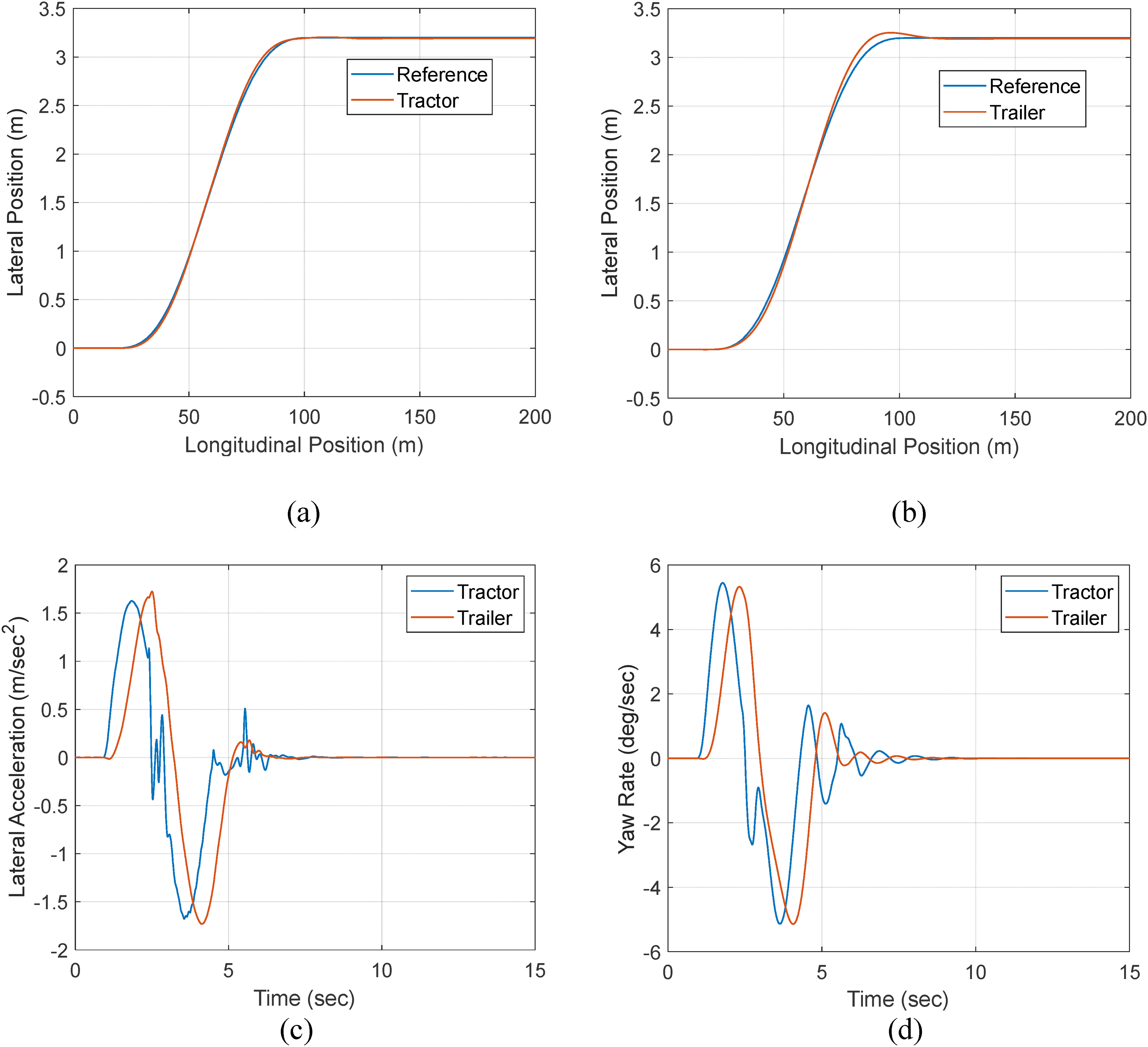
Tractor/semi-trailer directional performance determination using dynamic responses acquired from single lane-change (SLC) overtaking maneuver: (a) reference and actual tractor path; (b) reference and actual trailer path; (c) time-histories of tractor and trailer lateral acceleration; (d) time-histories of tractor and trailer yaw rate.
Figure 9(c) shows the time histories of the lateral acceleration at the CG of both the tractor and trailer. The maximum peak values of the lateral acceleration of the tractor and trailer are 1.677 and 1.729 m/s2, respectively. The above maximum peak values of the lateral acceleration indicate that the AHV operates within its linear lateral dynamic range. The RA measure of the AHV thus takes the value of 1.03, which is close to the desired value of 1.0. 55
Figure 9(d) illustrates the time histories of the yaw rate of both the leading and trailing units. The maximum peak values of the yaw rate of the tractor and trailer are 5.443°/s and 5.319°/s, respectively. As seen in the figure, each of the time histories of the yaw rates looks like a single-cycle sine wave, which is consistent with the published results achieved under similar obstacle avoidance maneuvers.56–58 Moreover, comparing the above maximum yaw rate values with those reported in these references, it may be deduced that yaw stability can be achieved for this AHV over the SLC overtaking maneuver. Table 4 summarizes the performance measures of the baseline tractor/semi-trailer combination acquired from the overtaking maneuver. Note that the term baseline tractor/semi-trailer combination implies that the vehicle system parameters take the values listed in Appendix 3.
Performance measures of the tractor/semi-trailer combination acquired from the simulation results under the single lane-change (SLC) overtaking maneuver.
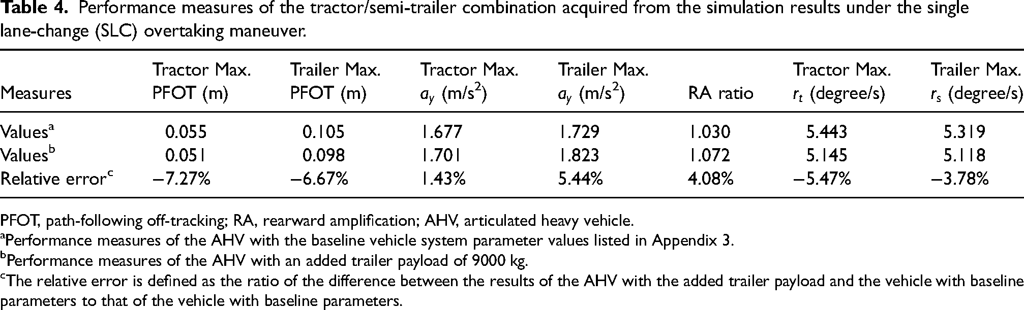
PFOT, path-following off-tracking; RA, rearward amplification; AHV, articulated heavy vehicle.
Performance measures of the AHV with the baseline vehicle system parameter values listed in Appendix 3.
Performance measures of the AHV with an added trailer payload of 9000 kg.
The relative error is defined as the ratio of the difference between the results of the AHV with the added trailer payload and the vehicle with baseline parameters to that of the vehicle with baseline parameters.
To find the root factors determining the performance measures listed in Table 4, we examine the tire dynamic states, steering, and driving actuation shown in Figure 10. Over the overtaking maneuver, under the control of the NLMPC controller, the steering actuation is applied on the tractor's front wheels to track the reference path. To follow the desired path and maintain lateral stability under the maneuver, the AHV needs to secure the required lateral forces from the road surface by manipulating tire slip angles. Figure 10(a) shows the time histories of slip angles of tractor front tires, tractor rear tires, and trailer tires, and Figure 10(b) illustrates the associated time history of the tractor front wheel steering angle. It is found that the time-history curve of the tractor front wheel steering angle takes an approximate single-cycle sine wave with a maximum peak value of 1.64°. This kinematic feature of the tractor front wheel steering angle determines the SLC paths of the tractor and trailer as shown in Figure 9(a) and (b), respectively.
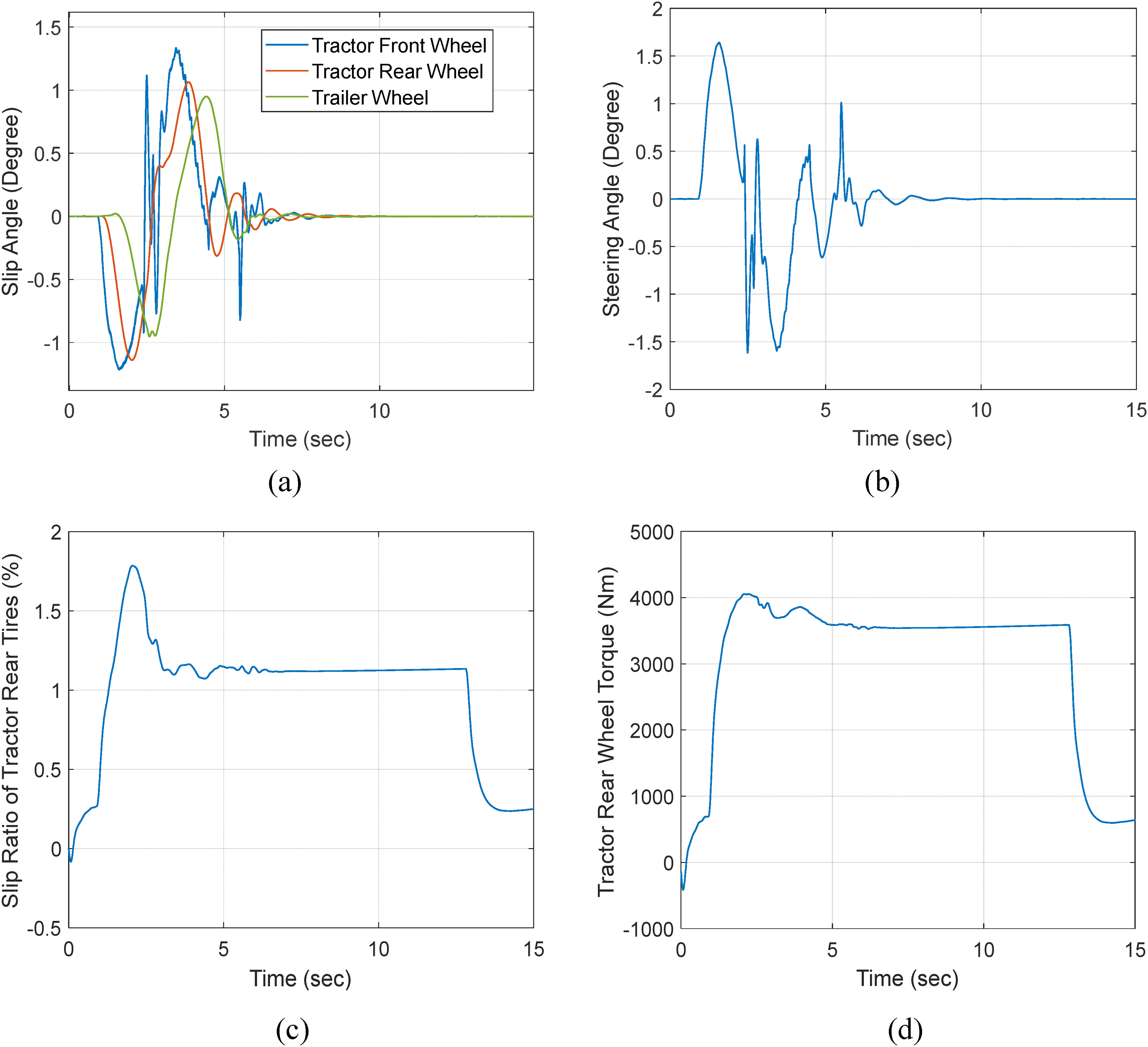
Tire dynamic states, steering, and driving actuation over single lane-change (SLC) overtaking maneuver: (a) time-histories of tire slip angles for both the leading and trailing units; (b) time-history of tractor front wheel steering angle; (c) time-history of longitudinal slip ratio of tractor rear tire; (d) time-history of driving torque on tractor rear wheel.
A close observation of Figure 10(a) discloses the following three facts: (a) each of the three tire slip angle curves looks more or less like a single-cycle sine wave, which is however out-phase in relation to the curve of tractor front wheel steering angle; (b) the maximum peak value of the three tire slip angle curves is <1.4°; (c) the amplitude of the respective single-cycle sine wave of tire slip angle curve drops from the tractor front tires, via the tractor rear tires, to the trailer tires. The first fact governs the timely varying cornering forces (in terms of direction and magnitude) on tractor front tires, tractor rear tires, and trailer tires in relation to the tractor front wheel steering angle. The second factor indicates that the AHV operates in the linear lateral dynamic range over the SLC maneuver, which confirms the previous linear lateral acceleration analysis shown in Figure 9(c). The third fact implies that the effect of the tractor front wheel steering actuation on controlling the PFOT measure of the tractor is stronger than on controlling the PFOT measure of the trailer. This fact well explains the difference between the PFOT measures of the leading and trailing units listed in Table 4.
Figure 10(c) and (d) shows the time history of the longitudinal slip ratio of the tractor rear tire and the time history of driving torque on the tractor rear axle, respectively. Interestingly, the shapes of the curves seen in the two figures look similar. As shown in Figure 10(c), the maximum longitudinal slip ratio of the tire is <1.8%. Thus, the longitudinal tire force and the slip ratio may be correlated by a linear relationship. This linear correlation may explain the shape similarity of the two curves. At the low longitudinal tire slip ratio shown in Figure 10(c), the rear tractor-driving wheels perform approximately pure rolling on the road surface. In addition, the maximum driving torque on the wheels is about 4,000 Nm, which is far below the powertrain torque capacity limitation listed in Table 3. Therefore, it may be deduced that the vehicle's forward speed can be well controlled by the NLMPC controller. Actually, as seen in Figure 8(a), the vehicle's forward speed well tracks the reference one over the SLC overtaking maneuver.
In this study, all computations are conducted by running Matlab 2021 on a laptop computer with a processor of Intel ® Core™ i5-8520 CPU@1.60 GHz. The computation time required for simulating the SLC maneuver is ∼3.64 s for the testing procedure requiring 5.0 s. It is found that the computation time increases with the increase of
A comparison between schemes with and without trailer trajectory-tracking control
This subsection compares the two NLMPC control schemes, that is, considering trajectory-tracking control for both the leading and trailing units and without considering trajectory-tracking control for the trailing unit, using the selected simulation results shown in Figure 11. Figure 11(a) shows the time histories of the trailer lateral position for both the schemes and the reference one. Without trailer tracking control, the maximum overshoot is 0.060 m, while the counterpart for the first scheme is 0.055 m. By introducing the trailer tracking control, the maximum overshoot is reduced by 9.1%.
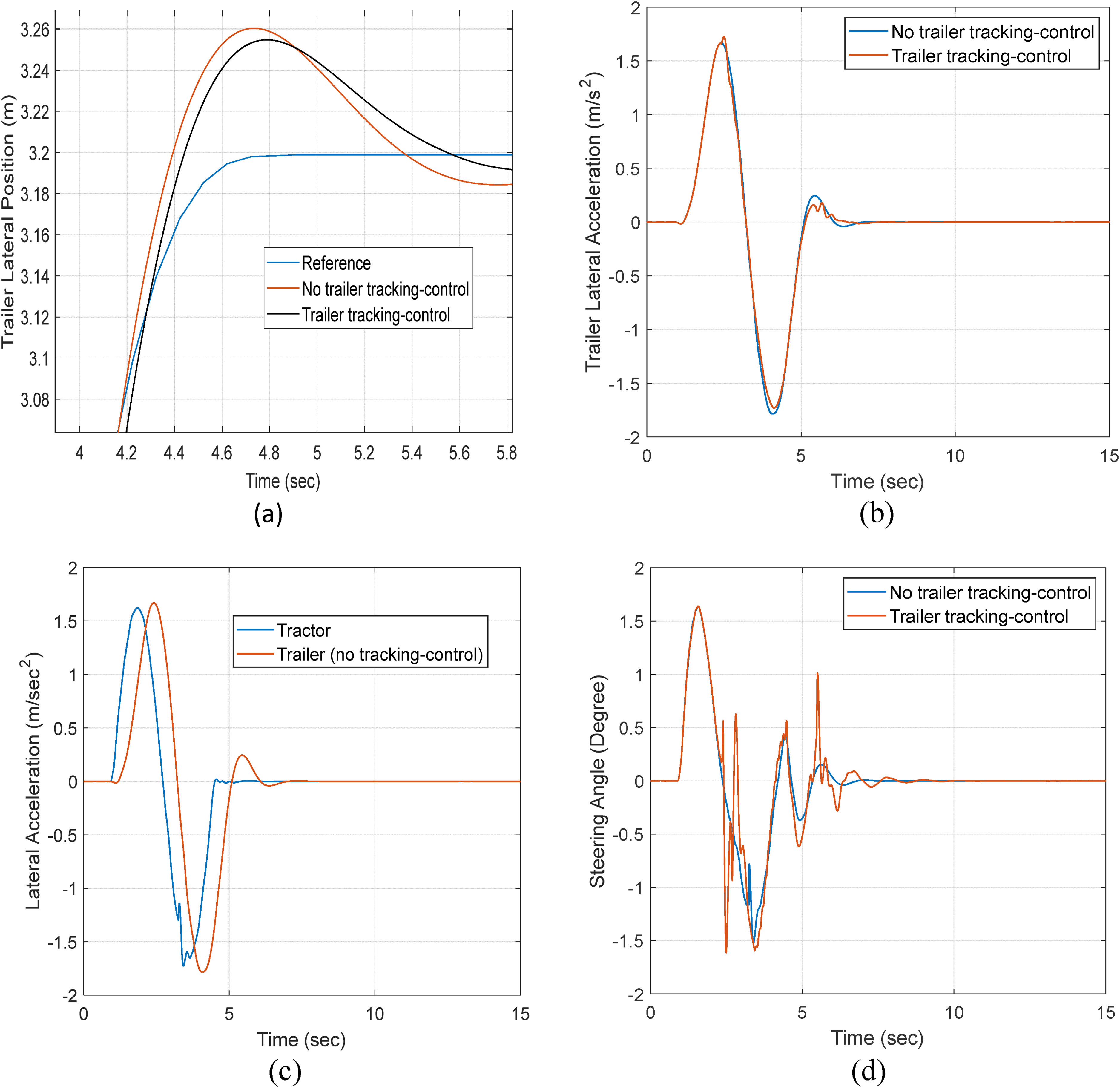
A comparison between schemes with and without trailer tracking control: (a) time histories of trailer lateral positions; (b) time histories of trailer lateral accelerations; (c) time histories of tractor and trailer lateral accelerations; (d) time histories of tractor front wheel steering angles.
Figure 11(b) compares the time histories of trailer lateral accelerations for the two cases over the maneuver. In the first case, the maximum peaking lateral acceleration is 1.729 m/s2, decreasing 3.03% from 1.783 m/s2, which is the counterpart of the second case. Figure 11(c) illustrates the time histories of lateral acceleration of the tractor and trailer for the second case. With the curves shown in this figure, we can determine the respective RA ratio of 1.033, which marginally increases from the corresponding measure of 1.030 for the first case.
Figure 11(d) shows the time histories of tractor front wheel steering angles for both cases. The root mean square (RMS) value for the first case is 0.64°, and the RMS for the second case is 0.58°. It is evident that the first control scheme gains improved performance at the expense of applying a larger tractor front wheel steering actuation effort.
The above benchmark indicates that compared with the scheme of tracking control for the tractor alone, the one of tracking control for both the leading and trailing units does improve the directional performance of the AHV over the SLC maneuver. However, the performance improvement is marginal. This phenomenon may be attributed to the fifth wheel (shown in Figure 4), which imposes a limited effect on the directional performance of AHVs. The attained benchmark result justifies the strategy for simultaneous autonomous driving and active trailer steering control reported in Rahimi et al. 6
A performance comparison of the tracking controller under different trailer payloads
To assess the robustness of the tracking controller under uncertain vehicle system parameters, the trailer is laden with an additional payload of 9000 kg. As mentioned previously, in the third case, for both the tractor and trailer, trajectory-tracking controls are performed so that the AHV tracks the reference motion trajectory (determined in the “Reference motion trajectory determination” section) over the SLC overtaking maneuver. The resulting vehicle performance measures derived from the dynamic responses acquired under the simulated SLC maneuver are listed in Table 4. Thus, the performance measures of the AHV equipped with the same tracking controller under two trailer payloads can be directly compared.
Figure 12(a) directly compares the time histories of the tractor lateral position of the AHV with two trailer payloads over the SLC overtaking maneuver. It appears that under the two different trailer payloads, the two curves shown in this figure are almost coincident. This implies that the given trailer payload variation poses a neglectable impact on the tractor's path-following performance. To have a close observation of the two curves shown in Figure 12(a), a local window accommodating the overshoots of the two curves is displayed in Figure 12(b). Obviously, the overshoot of the curve for the baseline trailer payload is larger than its counterpart for the trailer payload of 9000 kg.
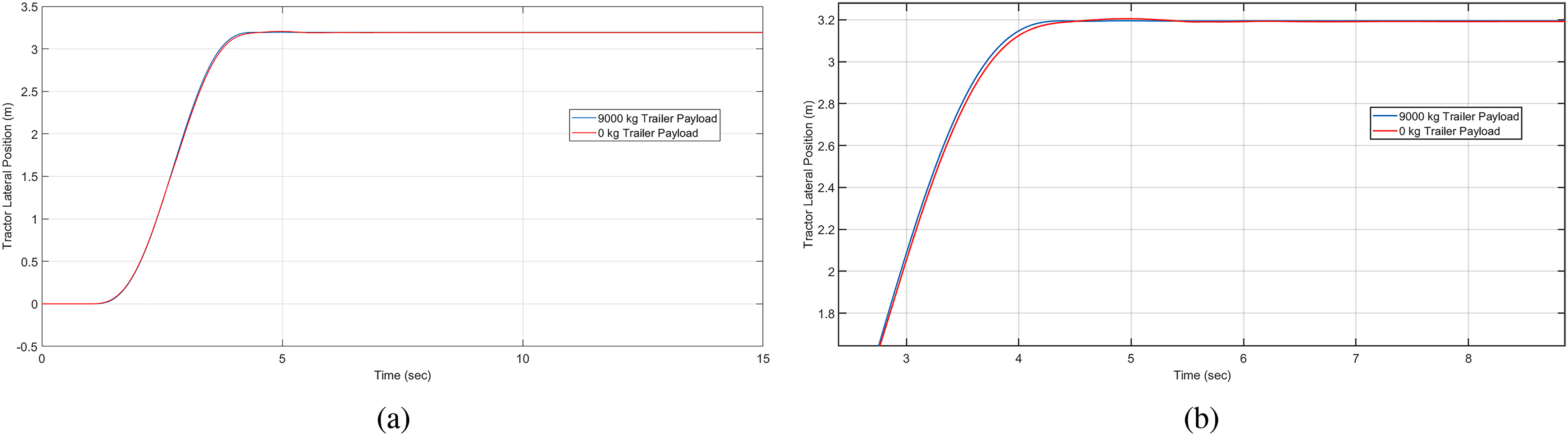
Time histories of tractor lateral position of the AHV with two different trailer payloads over the SLC overtaking maneuver: (a) overall time histories of the SLC maneuver, (b) partial time histories of the SLC maneuver.
To further examine the impact of trailer payload on the performance of the tracking controller, Figure 13 shows the dynamic responses of the AHV with the added trailer payload acquired under the simulated SLC overtaking maneuver. As shown in Figure 13(b), the maximum peak lateral acceleration of the tractor and trailer are 1.701 and 1.823 m/s2, increasing by 1.43 and 5.44% from their baseline values of 1.677 and 1.729 m/s2, respectively (see Table 4). The corresponding RA ratio is 1.072, increasing by 4.08% from its baseline value of 1.030. Obviously, as the trailer payload increases, the lateral stability of the vehicle degrades. Surprisingly, the maximum PFOT measures of the tractor and trailer dropped 7.27% and 6.67% from their baseline values (see Table 4). Moreover, the maximum yaw rate of the tractor and trailer was also reduced by 5.47% and 3.78% from their baseline counterparts. Thus, if the baseline vehicle with the tracking controller is treated as a reference, for the AHV with the added trailer payload and the same tracking controller, the well-accepted rule of thumb observation still exists: there is a trade-off between the lateral stability and path-following off-tracking performance of AHVs; in other words, the lateral stability of AHVs can be achieved at the expense of degradation of path-following off-tracking perform, and vice versa. 9 As listed in Table 4, with respect to the baseline vehicle, all the performance measures of the AHV with the added trailer payload of 9000 kg vary <7.5%. This reflects the high robustness of the tracking controller subject to the variation of trailer payload.
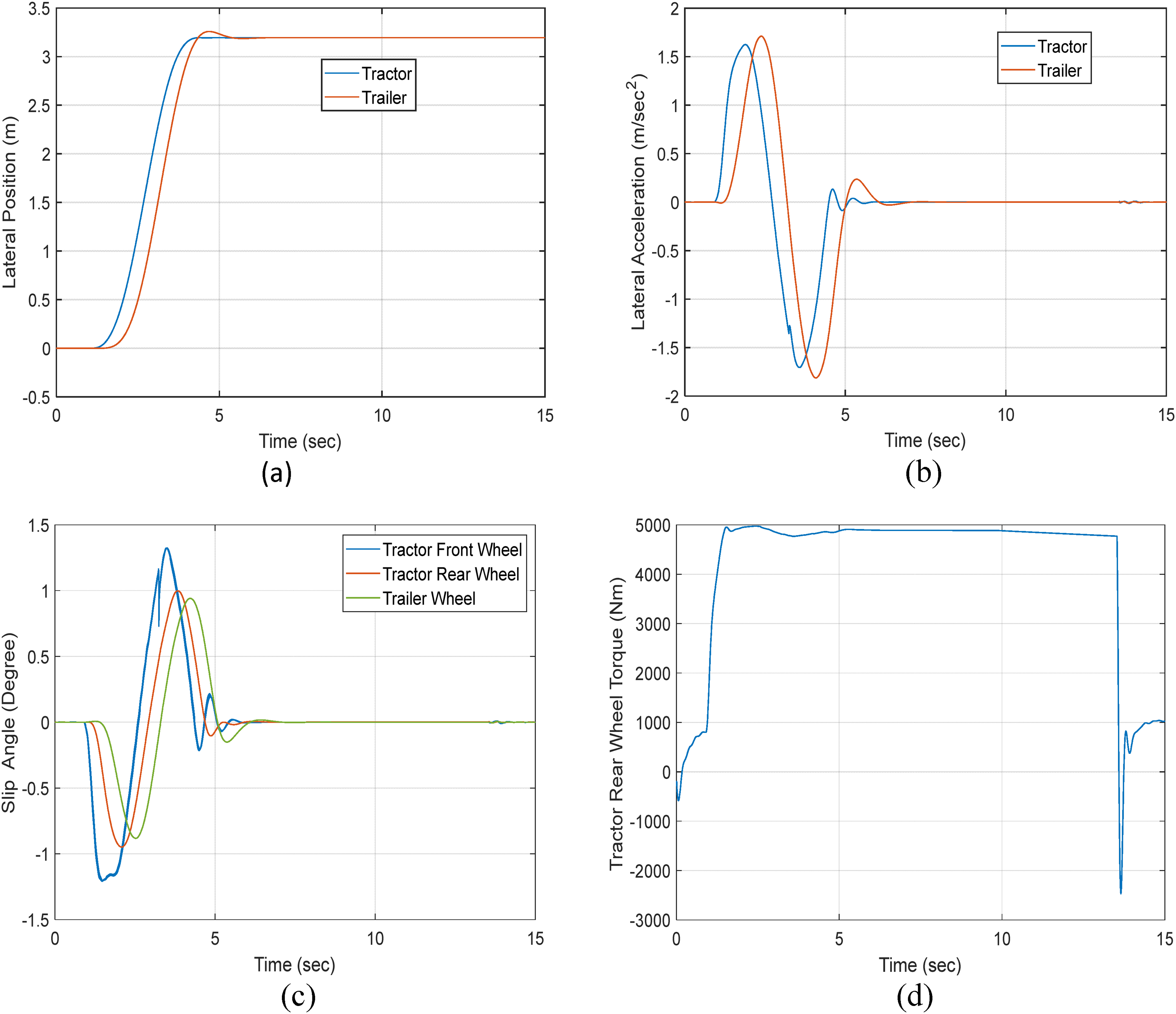
Dynamic responses of the tractor/semi-trailer with added trailer payload over the single lane-change (SLC) overtaking maneuver: (a) time-histories of tractor and trailer lateral position; (b) time-histories of tractor and trailer lateral acceleration; (c) time-histories of tire slip angles for both the leading and trailing units; (d) time-history of driving torque on tractor rear wheel.
Figure 13(c) shows the time histories of tire side slip angles for both the leading and trailing vehicle units. The three interesting dynamic features observed in Figure 10(a) can also be identified in Figure 13(c). The lateral tire dynamic similarity displayed in Figures 10(a) and 13(c) explains why the difference is <7.5% between the performance measures of the two cases (see Table 4). Figure 13(d) illustrates the time history of driving torque on the tractor's rear wheel. The peak driving torque is 5000 Nm, increasing 25% from its baseline value of 4000 km shown in Figure 10(d). By intuition, a larger driving torque is required for the tractor to tow a heavier trailer payload.
An assessment of the tracking controller under simulated double lane-change maneuver
Over the DLC maneuver, the vehicle's forward speed remains constant at 22.22 m/s (80 km/h), and the maximum lateral displacement is 3.194 m. The reference trajectory is shown in Figure 14(a). The selected dynamic responses of the AHV over the DLC maneuver are illustrated in Figure 14. To systematically analyze and discuss the simulation results shown in this figure, we take three steps: (a) comparing the simulation results acquired over the SLC and DLC maneuvers of the AHV with the trajectory-tracking control for both the tractor and trailer; (b) comparing the two trajectory-tracking control schemes; (c) evaluating the impact of the control parameter, that is, control horizon (
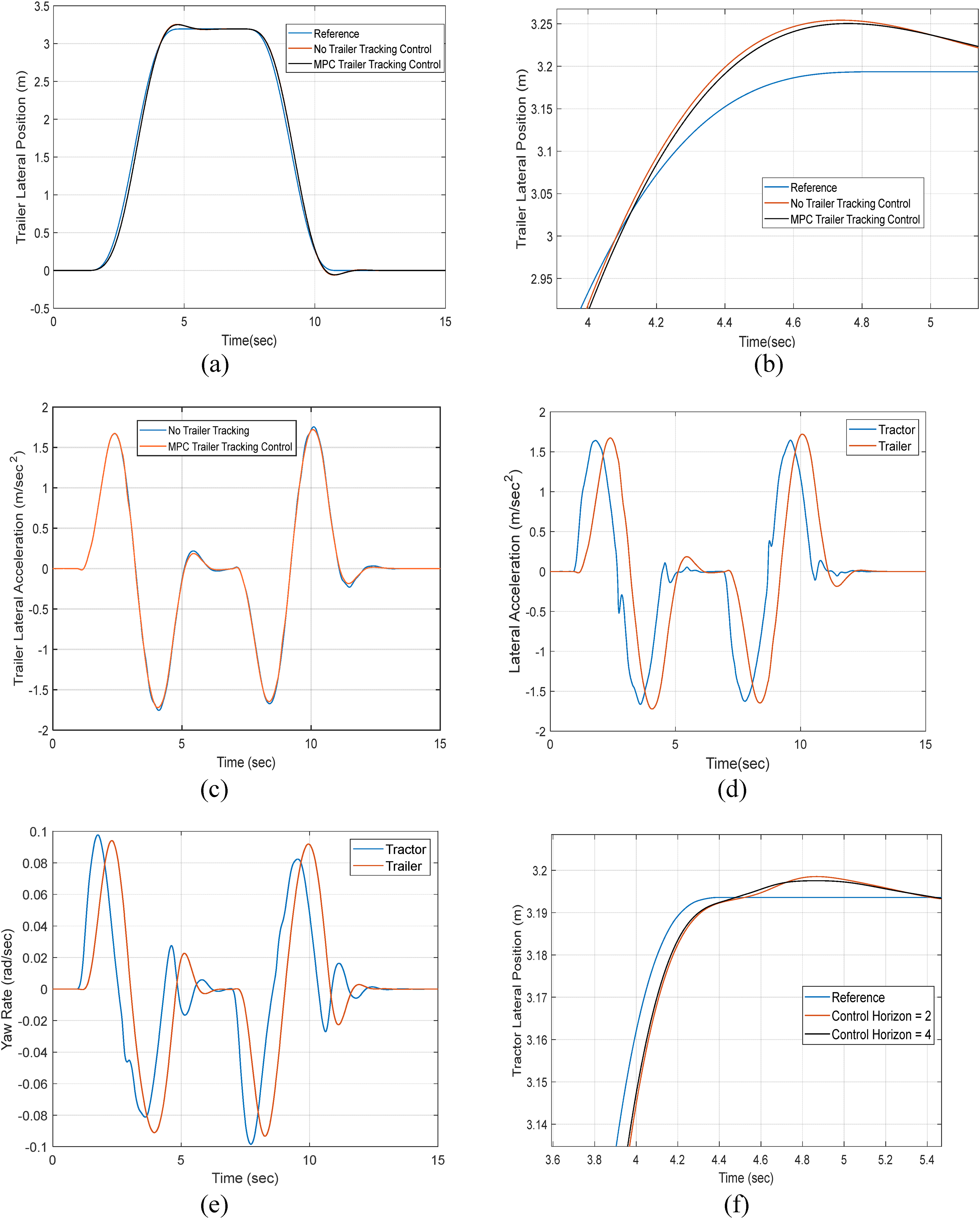
Dynamic responses of the tractor/semi-trailer over the DLC maneuver: (a) time histories of trailer lateral position; (b) partial time histories of trailer lateral position; (c) time histories of trailer lateral acceleration; (d) time histories of tractor and trailer lateral acceleration; (e) time histories of tractor and trailer yaw rate; (f) time histories of tractor of the AHV with two Hc values of the tracking-controller.
A close observation of Figure 14(d) and (e) discloses the fact that for each vehicle unit (i.e. either the tractor or the trailer), the respective curve (in terms of the time history of lateral acceleration and yaw rate) consists of approximately two single cycle sine waves. Interestingly, the second sine wave is approximately out-phase with respect to the first one. Comparing Figure 9(c) and (d) with Figure 14(d) and (e), respectively, we may assume that the DLC maneuver can be decomposed into two SLC maneuvers. The curves shown in Figures 9(a) and 14(a) justify this assumption. Actually, as shown in Figure 14(a), the AHV performs the first SLC, moving from the right lane to the left lane, then conducts the second SLC, switching from the right lane to the original left lane. Both the SLC and DLC scenarios shown in Figures 9(a) and 14(a) are typical obstacle avoidance maneuvers under highway operations.12,20 It is indicated that the RA ratio is one of the most important performance indicators of AHVs under high-speed evasive maneuvers.9,11 The RA measure reflects both the lateral stability and path-following performance of an AHV over a high-speed obstacle avoidance maneuver. Conventionally, the RA ratio is defined and measured over an SLC maneuver. 37 For the DLC maneuver shown in Figure 14(a), we define and measure the RA ratio over the first and second SLC maneuvers independently based on the simulation results shown in Figure 14(d). Table 5 lists the associated performance measures of the tractor/semi-trailer over the DLC maneuver. As listed in the table, the larger RA ratio (i.e. RA = 1.046) occurs over the second SLC of the DLC maneuver. Compared with the RA measure for the typical SLC maneuver (i.e. RA = 1.030) listed in Table 4, the counterpart measure (i.e. RA = 1.046) for the DLC maneuver only increases by 1.6%. Thus, under the two different high-speed obstacle avoidance maneuvers, the respective RA measures are excellently matched. This implies that the tracking controller behaves very robustly under the two different maneuvers.
Performance measures of the tractor/semi-trailer combination acquired from the simulation results under the DLC maneuver.
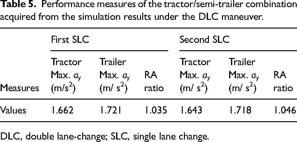
DLC, double lane-change; SLC, single lane change.
The simulation results shown in Figure 14(b) and (c) are used to examine the performance of the two trajectory-tracking control schemes (i.e. trajectory-tracking control for the tractor alone and for both vehicle units) over the DLC maneuver. For both the control schemes, Table 6 lists the maximum trailer PFOT (as seen in Figure 14(b) and the maximum trailer lateral acceleration (as shown in Figure 14(c)). As listed in the table, compared with the scheme of trajectory-tracking control for both the vehicle units, the trajectory-tracking control for the tractor alone increases the maximum trailer path-following off-tracking (PFOT) by 8.8% and the maximum trailer lateral acceleration by 2.0%. These comparison results based on the DLC maneuver achieve good agreement with those based on the SLC maneuver discussed in a comparison between schemes with and without trailer trajectory-tracking control.
Performance comparison of the two trajectory-tracking control schemes based on the simulation results of the trailer under the DLC maneuver.
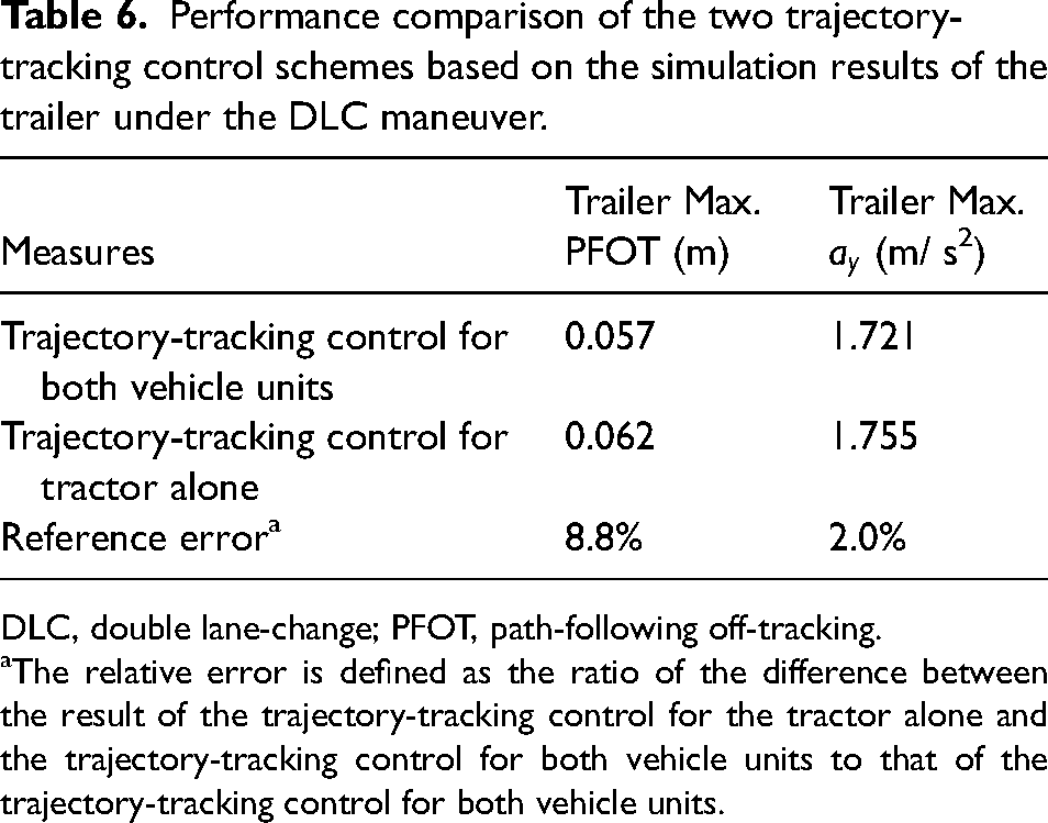
DLC, double lane-change; PFOT, path-following off-tracking.
The relative error is defined as the ratio of the difference between the result of the trajectory-tracking control for the tractor alone and the trajectory-tracking control for both vehicle units to that of the trajectory-tracking control for both vehicle units.
To examine the effect of control horizon (
The above simulation results demonstrate the robust performance of the proposed tracking controller under the severe DLC maneuver.
Conclusions
This paper proposes a design of a tracking controller for AAHVs using an NLMPC technique. To design the NLMPC controller, a new structured nonlinear 7-DOF tractor/semi-trailer model is developed, which consists of the sub-models of tractor and trailer rigid-bodies, Dugoff tire, wheel, and a simplified powertrain. Considering the trajectory-tracking control for both the leading and trailing units, we establish the kinematics for tractor/semi-trailer path-tracking. In the formulation of the NLMPC controller design, the constraints reflecting associated vehicle physical limits and design requirements, for example, ride comfort, time-efficient driving, collision-free, etc., are imposed. To evaluate the proposed tracking controller, the parameterized reference motion trajectory tailored from the SLC testing maneuver by ISO-14791 is introduced. The robustness of the tracking controller is examined through numerical simulations under both the SLC and a DLC maneuver and considering different trailer payloads.
The co-simulation built upon the Matlab/Simulink-TruckSim environment is conducted to examine the NLMPC tracking-controller design. Simulation results disclose the following insightful findings: (a) over the specified SLC overtaking maneuver, the tracking controller can well control the AHV in the linear lateral and longitudinal dynamic ranges so that the vehicle can achieve good path-following performance and lateral stability; (b) over the overtaking maneuver, to respond to the tractor front wheel steering actuation, the responding efforts of the tractor and trailer tires in terms of the amplitude of tire slip angle are different, which decrease from the tractor front tires, via the tractor rear tires, to the trailer tires; (c) due to the difference of the responding efforts of the tractor and trailer tires in terms of tire slip angles, the tractor's path-following performance is better controlled than that of the trailer; (d) the tracking controller shows high robustness under varied trailer payload and different high-speed obstacle avoidance maneuvers. To further assess the NLMPC controller design, a benchmark comparison is conducted between the two control schemes: (i) considering tracking control for both the leading and trailing vehicle units and (ii) considering tracking control for the leading vehicle unit alone. Numerical experiments demonstrate that compared with the second scheme, the first one (i.e., the proposed design) can achieve better overall performance in terms of the PFOT measures and lateral stability at the expense of larger tractor front wheel steering actuation. It is expected that the proposed NLMPC tracking controller will be validated using in-vehicle field/road tests in the near future.
Footnotes
Declaration of conflicting interests
The authors declared no potential conflicts of interest with respect to the research, authorship, and/or publication of this article.
Funding
The authors disclosed receipt of the following financial support for the research, authorship, and/or publication of this article: This research was financially supported by the Natural Sciences and Engineering Research Council of Canada (grant number RGPIN-2019-05437).
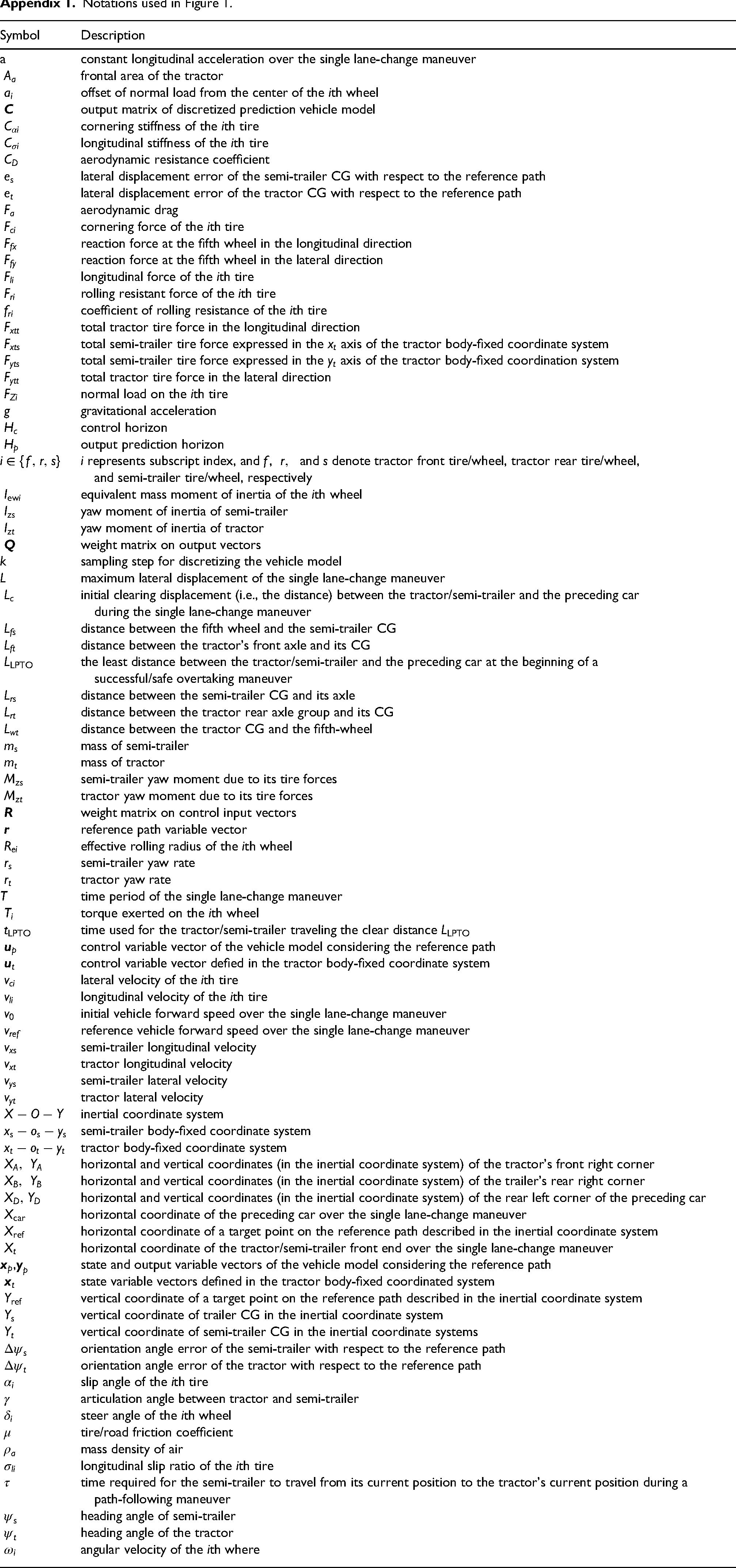
Notations used in Figure 1.
| Symbol | Description |
|---|---|
| a | constant longitudinal acceleration over the single lane-change maneuver |
| frontal area of the tractor | |
| offset of normal load from the center of the | |
| output matrix of discretized prediction vehicle model | |
| cornering stiffness of the tire | |
| longitudinal stiffness of the tire | |
| aerodynamic resistance coefficient | |
| lateral displacement error of the semi-trailer CG with respect to the reference path | |
| lateral displacement error of the tractor CG with respect to the reference path | |
| aerodynamic drag | |
| cornering force of the tire | |
| reaction force at the fifth wheel in the longitudinal direction | |
| reaction force at the fifth wheel in the lateral direction | |
| longitudinal force of the tire | |
| rolling resistant force of the tire | |
| coefficient of rolling resistance of the tire | |
| total tractor tire force in the longitudinal direction | |
| total semi-trailer tire force expressed in the axis of the tractor body-fixed coordinate system | |
| total semi-trailer tire force expressed in the axis of the tractor body-fixed coordination system | |
| total tractor tire force in the lateral direction | |
| normal load on the tire | |
| gravitational acceleration | |
| control horizon | |
| output prediction horizon | |
| represents subscript index, and , denote tractor front tire/wheel, tractor rear tire/wheel, and semi-trailer tire/wheel, respectively | |
| equivalent mass moment of inertia of the wheel | |
| yaw moment of inertia of semi-trailer | |
| yaw moment of inertia of tractor | |
|
|
weight matrix on output vectors |
| k | sampling step for discretizing the vehicle model |
| L | maximum lateral displacement of the single lane-change maneuver |
| initial clearing displacement (i.e., the distance) between the tractor/semi-trailer and the preceding car during the single lane-change maneuver | |
| distance between the fifth wheel and the semi-trailer CG | |
| distance between the tractor's front axle and its CG | |
| the least distance between the tractor/semi-trailer and the preceding car at the beginning of a successful/safe overtaking maneuver | |
| distance between the semi-trailer CG and its axle | |
| distance between the tractor rear axle group and its CG | |
| distance between the tractor CG and the fifth-wheel | |
| mass of semi-trailer | |
| mass of tractor | |
| semi-trailer yaw moment due to its tire forces | |
| tractor yaw moment due to its tire forces | |
|
|
weight matrix on control input vectors |
| reference path variable vector | |
| effective rolling radius of the wheel | |
| semi-trailer yaw rate | |
| tractor yaw rate | |
| T | time period of the single lane-change maneuver |
| torque exerted on the wheel | |
| time used for the tractor/semi-trailer traveling the clear distance | |
| control variable vector of the vehicle model considering the reference path | |
| control variable vector defied in the tractor body-fixed coordinate system | |
| lateral velocity of the tire | |
| longitudinal velocity of the tire | |
| initial vehicle forward speed over the single lane-change maneuver | |
| reference vehicle forward speed over the single lane-change maneuver | |
| semi-trailer longitudinal velocity | |
| tractor longitudinal velocity | |
| semi-trailer lateral velocity | |
| tractor lateral velocity | |
| inertial coordinate system | |
| semi-trailer body-fixed coordinate system | |
| tractor body-fixed coordinate system | |
| horizontal and vertical coordinates (in the inertial coordinate system) of the tractor's front right corner | |
| horizontal and vertical coordinates (in the inertial coordinate system) of the trailer's rear right corner | |
| horizontal and vertical coordinates (in the inertial coordinate system) of the rear left corner of the preceding car | |
| horizontal coordinate of the preceding car over the single lane-change maneuver | |
| horizontal coordinate of a target point on the reference path described in the inertial coordinate system | |
| horizontal coordinate of the tractor/semi-trailer front end over the single lane-change maneuver | |
| , | state and output variable vectors of the vehicle model considering the reference path |
| state variable vectors defined in the tractor body-fixed coordinated system | |
| vertical coordinate of a target point on the reference path described in the inertial coordinate system | |
| vertical coordinate of trailer CG in the inertial coordinate system | |
| vertical coordinate of semi-trailer CG in the inertial coordinate systems | |
| orientation angle error of the semi-trailer with respect to the reference path | |
| orientation angle error of the tractor with respect to the reference path | |
| slip angle of the tire | |
| articulation angle between tractor and semi-trailer | |
| steer angle of the wheel | |
| tire/road friction coefficient | |
| mass density of air | |
| longitudinal slip ratio of the tire | |
| time required for the semi-trailer to travel from its current position to the tractor's current position during a path-following maneuver | |
| heading angle of semi-trailer | |
| heading angle of the tractor | |
| angular velocity of the where |
Appendix 2. A simplified powertrain model
Figure 15 shows the simplified powertrain system, which consists of an internal combustion (IC) engine or an electric motor with an output torque
In this study, a diesel engine is adopted, and its output torque (
Given the powertrain shown in Figure 15, the equivalent mass moment of inertia of the driving wheel is determined by
Parameter values of seven degrees of freedom (7-DOF) and TruckSim tractor/semi-trailer models.
| 3.2 m2 | |
| 0.66 | |
| {200,000 × 2, 50,000 × 8, 40,000 × 12} N/rad | |
| {270,000 × 2, 85,000 × 8, 65,000 × 12} N/unit slip | |
| {0.0041, 0.0041, 0.0041} | |
| 150,000 kg·m2 | |
| 19,965 kg·m2 | |
| 5.5 m | |
| 1.385 m | |
| 2.4 m | |
| 4.25 m | |
| 4.25 m | |
| 7807 kg | |
| 7878 kg | |
| {0.51, 0.51, 0.51} m | |
| 0.5 | |
| 1.206 kg/m3 |