
Abstract
The heavy-haul train has a series of characteristics, such as the locomotive traction properties, the longer length of train, and the nonlinear train pipe pressure during train braking. When the train is running on a continuous long and steep downgrade railway line, the safety of the train is ensured by cycle braking, which puts high demands on the driving skills of the driver. In this article, a driving curve generation method for the heavy-haul train based on a neural network is proposed. First, in order to describe the nonlinear characteristics of train braking, the neural network model is constructed and trained by practical driving data. In the neural network model, various nonlinear neurons are interconnected to work for information processing and transmission. The target value of train braking pressure reduction and release time is achieved by modeling the braking process. The equation of train motion is computed to obtain the driving curve. Finally, in four typical operation scenarios, comparing the curve data generated by the method with corresponding practical data of the Shuohuang heavy-haul railway line, the results show that the method is effective.
Introduction
Automatic train operation (ATO) has been widely used in urban rail transit in recent years. However, there are still some difficulties in applying ATO to the heavy-haul train (HHT) because of some characteristics of HHT, such as the locomotive traction properties, the train is long, and nonlinear train pipe pressure during train brake operation, which are mainly dependent on air braking on the continuous long and steep downgrade and nonlinear train pipe pressure when reducing the speed of vehicles along the train. Due to the nonlinear complexity of dynamic operation, the driver must follow a given driving curve when driving an HHT to ensure the operation safety. The given driving curve is generally obtained from field driving data of many experienced drivers. However, since there are various types of locomotives and marshaling, it is difficult to get a range of driving curves for different scenarios. The driver therefore needs to control the train using his own experience, although he may not always make good choices, for reasons which include the labor intensity of the job and driver fatigue, increasing the risk of accidents. To resolve this issue, a driving curve generation method has been put forward which can generate the driving curve of an HHT based on an artificial neural network (NN).
In recent years, much research on the train operation of rail transit systems has been carried out using different methods. For example, a model selection technique has been introduced to optimize the braking model and identify the parameters of urban rail transit systems in the field of ATO for urban rail transit, but the nonlinearity makes it hard for HHT. Based on system parameter identification theory, the ATO model has been obtained from field data.1,2 Self-adaptive fuzzy control technique and fuzzy logic self-tuning of scale gene have been applied to the speed of ATO in the urban rail transit system.3,4 However, the complexity and nonlinearity of dynamic operation make it difficult to directly control the HHT by ATO. In the HHT field, considering the interaction force between vehicles and the control difficulties of HHT, a decentralized control model has been employed to the control of the vehicle’s speed. 5 But, how to achieve the control speed is not considered. A predictive control model has been introduced to study the whole HHT operation process and control the train speed.6–8 The control of train speed is realized by the constructed models in the published work, but no specific operational control parameter is given for the driver.9–12 According to requirements of the speed limits in the different points of slope changing, the backing-off algorithm is used to calculate the HHT operation curve, but it needs to be repeated to calculate the difference value between the train practical speed and the limit speed in the point of slope changing and judging the rationality of driving curve simultaneously. 13 Therefore, a driving curve generation method for HHT based on an NN is proposed, which mainly focuses on the continuous long and steep downgrade to solve this problem and obtain the train braking pressure reduction (BPR). Providing that the NN model is suitable, the model is trained by field driving data with improved training algorithm, and then the expected target value of train BPR and release time can be obtained by inputting the real-time parameters into the model in the generation process. Combining obtained train braking force with the traction and resistance of the HHT, the driving curve in different railway line scenarios can be achieved by computing the equation of train motion. The curves are compared with different practical driving curves.
Modeling of HHT driving curve based on NN
The train driving curve generation model must ensure both the safety requirements and the efficient operation of the HHT. When an HHT is running on the continuous long and steep downgrade, it is necessary to generate the train driving curve rapidly, efficiently, and accurately based on the synthesized analysis of the real-time information, such as train position, speed, the length, gradient, and the speed limit of the railway line.
Model of train
Both the influence of the air brake function on the continuous long and steep downgrade and the section with difficult operation under a three-aspect block system should be given particular consideration in the operation process of the HHT. The train pipe pressure is 500/600 kPa without using the air brake function. The pressure of the train pipe is reduced to slow the train speed when using air braking control. In addition, in order to ensure the braking ability next time, the pressure of the train pipe should recover to constant by air charging when finishing air brake. Because the whole control process needs sufficient time, improper operation of the driver may cause the train to be out of control with weak braking ability. To cope with this problem, the following scenario will be studied.
Assume that there are two or more long and steep downgrades, and the slope length is not less than 2 km when the train is running on the railway line. The corresponding HHT model and running scenario are described in equations (1) and (2)
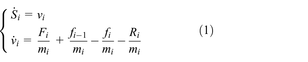
where i indicates the ith vehicle and S, v, and m denote the running distance, speed, and mass of the vehicles, respectively. F is traction or braking force, f is the interaction force between the ith and (i + 1)th vehicle and R is the resistance of the ith vehicle. The distance and speed of the train can be calculated by the forces
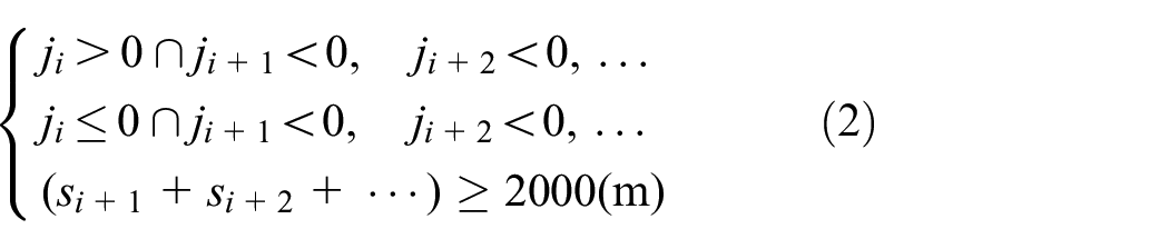
where j(‰) is the gradient, s is the slope length, and i represents the ith slope of the railway line. The equation describes that the downslope number is more than 2, and the slope length is more than 2000 m when the train is on the upslope or downslope.
Equation of train motion
In the assumption scenario, there are three kinds of force, such as traction, braking force, and resistance which always exist in the operation process. There is also rotary motion when the train is in translational motion, in view of running time and distance, equation (1) can also be written as

where c is the unit resultant force of the train; S, v, and t denote the distance, speed, and time, respectively; and

where M is the mass of the whole train, I is the rotational inertia of the rotary motion part,
Modeling of NN
A NN consists of several neurons that are connected with different weights to process and transfer information. An error backpropagation (BP) NN is easy to implement and widely used in the function approximation, pattern recognition, and classification. The structure of BP NN is so simple, but with proper hidden layers and nodes, the BP NN can approximate any nonlinear mapping relations with good simplicity and generalization ability and keep good simplicity of the algorithm at the same time. The authors use the method of improved BP NN.
The NN model is a multilayer structure and each layer has output vectors, an error vector and weight matrix. So far, there are various training function algorithms, such as gradient descent, 14 conjugate gradient, 15 Levenberg–Marquardt, Broyden–Fletcher–Goldfarb–Shanno (BFGS) quasi-Newton algorithm 17 and some improved training methods.18–20 The improved BP NN has a three-layer structure, the f1 is a tan-sigmoid function, and the f2 is a linear function.
The output of the NN can be described as

where
In order to make the NN effective, the related data must be normalized for processing, which make the value of all parameters in the range of [0, 1]. The weight values of the NN model are adjusted by the limited-memory Broyden–Fletcher–Goldfarb–Shanno (L-BFGS) quasi-Newton training algorithm, which is an improved learning algorithm of the BFGS algorithm. It does not need to compute the Hessian matrix and it updates the weight values (xk+1) by equation (6)

where
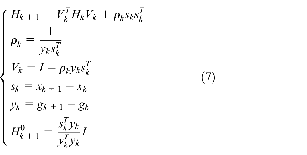
where (sk, y
k
) is the curvature information, ρk and Vk are intermediate variables, and H0 is the original matrix which is known. The L-BFGS algorithm updates
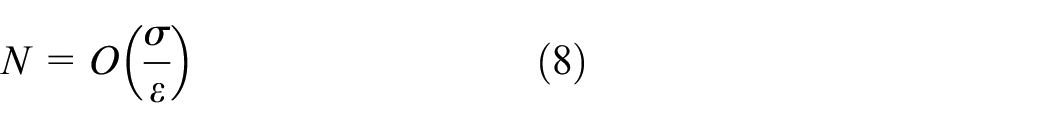
The node number of the hidden layer is determined by the practical scenario and it may affect the precision of the NN. It may have a long training time or it could be over-fitted with too many nodes. The training time and precision will be affected if the node number is too small. To avoid over-fitting, the training sample size N should meet the condition as
where
The training and validation sample is randomly selected from the whole field data. The node number n of the hidden layer can be determined by the following equation

where a is a constant between 0 and 10, u is the node number of the input layer, z is the node number of the output layer, N is the training sample size, and
In the NN training process, choosing an error as the given standard, the error function is defined by equation (10) to determine whether the training meets the precision requirement

where
Based on the operation and driving characteristics of the HHT, the NN model is established to generate the driving curve. Using the field data to get the mapping relationship, a corresponding NN model can be achieved to control the train using driver’s experience. The modeling data are collected from practical driving data. The modeling data group based on Shuohuang heavy-haul railway line is conducted. The total Shuohuang heavy-haul railway line covers a length of 600 km. The maximum gradient of downslope is 12‰. The maximum speed limit is 80 km/h.
Driving curve generating algorithm of the train
In the process of train driving curve generation, first, it is judged whether the HHT meets the model conditions; if the train is running on the upslope railway line, the train does not need cycle braking. As long as the model satisfies the requirements, the corresponding practical time parameters are put into the trained NN model.
The parameters are railway line speed limit vlim, gradient j, the weight of the HHT G, length of the train L, train speed v, preceding train distance S, and reaction time of driver t1. Then, the two outputs’ target value of train BPR r and release time t2 are obtained by the NN model. The modeling process based on the NN is shown in Figure 1.
Step 1. Collect and process the normalized train driving data, which should be sufficient to make function approximation to reduce the error.
Step 2. Construct the applicable conditions of the generation model, which is based on the analysis of the field operation and characteristics of the HHT. The conditions are shown in equation (2).
Step 3. Confirm and select the parameters that can represent the characteristics of the HHT as the input and output data of the NN model. While decreasing the node number of the hidden layer, the training time will be shorter, but the precision of the fitting will be lower. According to the NN parameters of each layer obtained above, and for the balance of training time and precision of the fitting, the corresponding NN model is built. There are 7 nodes consisting of one input layer and one output layer with 2 nodes, and 11 nodes consisting of one hidden layer by trial and error. So the structure of the NN is (7 × 11 × 2).The training sample and validation sample are selected randomly.
Step 4. Take the railway line speed limit, gradient, the weight of the HHT, length of the train, train speed, preceding train distance, and reaction time of the driver as the input data of the NN; the input parameters are listed as follows:
x 1: vlim (railway line speed limit);
x 2: j (gradient);
x 3: G (weight of HHT);
x 4: L (length of the train);
x 5: v (train speed);
x 6: S (preceding train distance);
x 7: t1 (reaction time of driver).
And take the target value of train BPR and release time as the output data:
y 1: r (target value of train BPR);
y 2: t2 (release time of the train).
Step 5. Using the self-learning and adaptive ability of the NN, the L-BFGS quasi-Newton algorithm is selected to train the NN using the field data.

Flow of the NN modeling.
The driving curve generation process for the HHT based on the NN is shown in Figure 2.

Flow of driving curve generation of HHT based on NN.
The driving curve is obtained by the outputs of the NN together with the train motion equation. The final driving curve cannot be obtained until the results meet the requirements, by which the stability and robustness of the process are enhanced, and the error and time delay are reduced.
Step 1. According to the status of HHT operation, if the status meets the constraint conditions of the model, then go to the next step. Otherwise, continue step 1. The constraint conditions of the model are
Step 2. Collect and process the practical time parameters of the train; vlim, j, G, L, v, S, t1; like the training sample; judge the kinds of conditions and input the data obtained into the corresponding trained NN model.
In view of the characteristics of HHT and the difficult problem of generating the driving curve of HHT, the authors establish the four typical operation scenarios. The first operation scenario is that a train will stop at the station along a continuous downslope with initial downslope. The second operation scenario is that a train will stop at the station along a continuous downslope with initial upslope. The third operation scenario is that a train will run along a very steep slope with initial downslope. The fourth operation scenario is that a train will run along a very steep slope with initial flat slope.
The data describe the process of cycle braking and train operation. The corresponding railway line speed limit, gradient, the weight of train, the length of the train, driver reaction time, and release time with different train BPRs are shown in Table 1.
Training data of four operation scenarios.

BPR: braking pressure reduction.
Figure 3 denotes 200 groups of training data of scenario 1 and includes the data of train BPR, speed, and preceding train distance, and Figure 4 denotes that the randomly selected test data have been processed to describe the error of the NN modeling process. With the principle that validation data group should equal or be smaller than the training data group, 180 groups of data are chosen as validation data. The maximum error is 0.72, and the mean error is 2.2%.
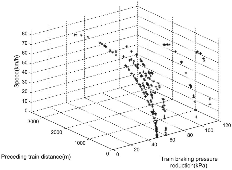
Training data of scenario 1.

Test data error of scenario 1.
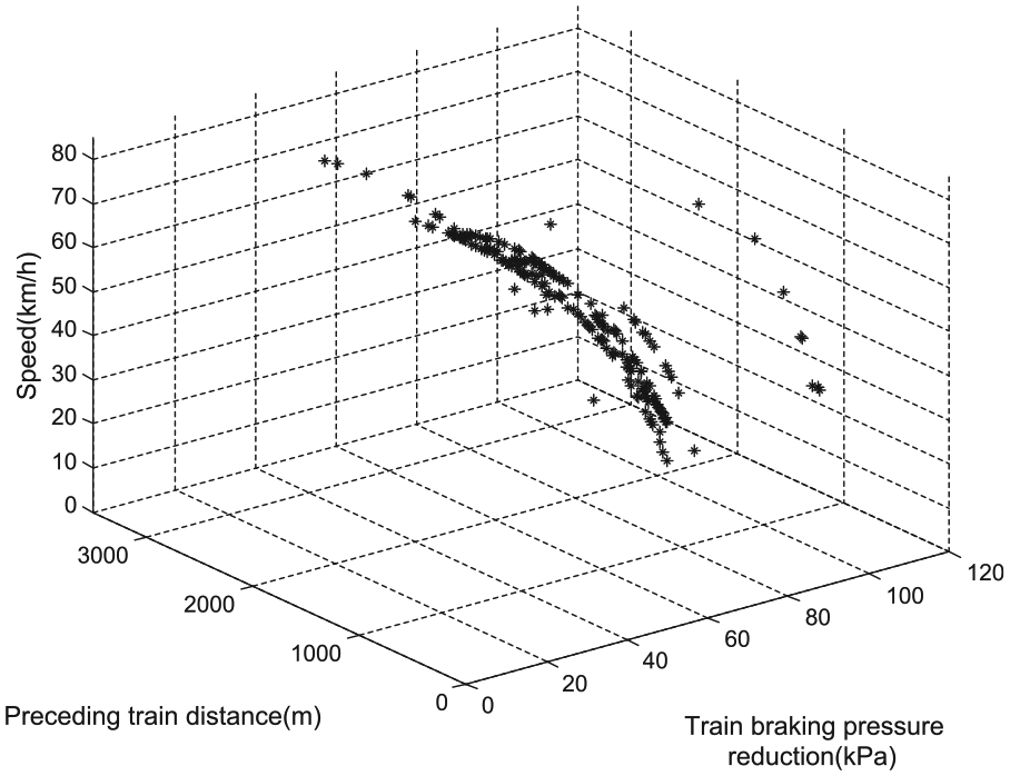
Figure 5 denotes 186 groups of training data of scenario 1 and includes the data of train BPR, speed, and preceding train distance, and Figure 6 denotes that 100 groups of data are chosen as validation data. The maximum error is 0.6, and the mean error is 1.8%.

Training data of scenario 2.

Test data error of scenario 2.
Figure 7 denotes 200 groups of training data of scenario 3 and includes the data of train BPR, speed, and preceding train distance, and Figure 8 denotes that 180 groups of data are chosen as validation data. The maximum error is 0.65, and the mean error is 2.8%.

Training data of scenario 3.

Test data error of scenario 3.
Figure 9 denotes 203 groups of training data of scenario 4 and includes the data of train BPR, speed, and preceding train distance, and Figure 10 denotes that 100 groups of data are chosen as validation data. The maximum error is 0.5, and the mean error is 1.7%.
Training data of scenario 4.

Test data error of scenario 4.
Step 3. Get the outputs r and t2 from the NN model y1, y2 and normalize the parameters. The output is written as

where k = 1, 2; i = 1,…, 7. The parameters have the same meaning as equation (5); the subscript indicates the NN layers. Then, calculate the train forces which are important in calculating the equation of train motion.
Step 4. Based on the target value, train BPR r, release time t2, and other known parameters obtain the train resultant force. Next, calculate the running speed, time, and distance for generating the train driving curve.
When the speed of the locomotive is confirmed, the locomotive traction is set as 90% of the maximum traction with the corresponding speed. Train resistance consists of basic resistance and additional resistance due to the curve and tunnel. Train air braking force is formed by the friction of the brake shoe. Calculation equations of the locomotive traction, train resistance, and braking force can be written as

where
The equivalent braking ratio is full and the
Value of coefficient of normal braking

When the train is braking, the train braking distance (BD) can be written as
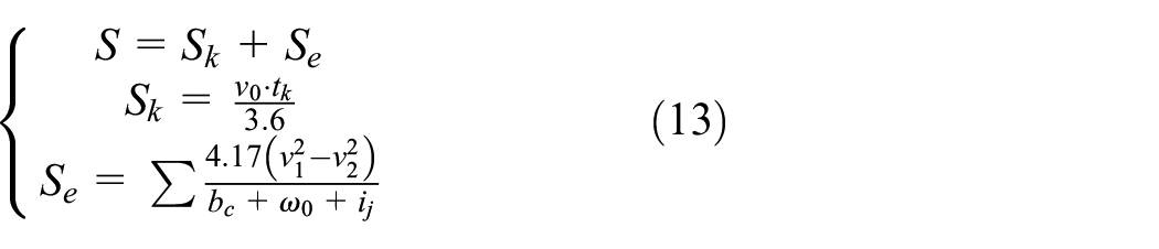
where S is the distance of train braking, which consists of the running distance
If the results meet the requirements, record the driving curve; otherwise, repeat the above steps. The constraints of the HHT are integrated as follows

where r is the target value of train BPR by air braking,
Step 5. The evaluation indices of the train under different conditions can be calculated, such as expectation and variance of speed difference, BD, and mean speed.
Step 6. Judge the driving curve results and end the process if it meets the requirements; otherwise, rerun the process.
Simulation analysis
Based on four typical operation scenarios, four cases based on Shuohuang heavy-haul railway line are conducted as examples. The generation of the driving curve is achieved by MATLAB simulation software programming. The simulation parameters are shown in Table 3.
Simulation parameters of the model.

The railway line parameters, length of slope, gradient, and cumulative distance of the four operation scenarios are shown in Tables 4–7, respectively.
Simulation railway line parameters of scenario 1.

Simulation railway line parameters of scenario 2.

Simulation railway line parameters of scenario 3.

Simulation railway line parameters of scenario 4.

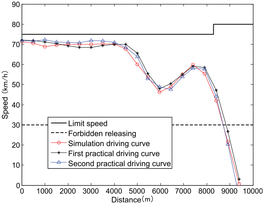
The simulation driving curve (SDC), first practical driving curve (FPDC), and second practical driving curve (SPDC) of four operation scenarios are shown in Figures 11–14, respectively.

Simulation and practical HHT driving curves of scenario 1.
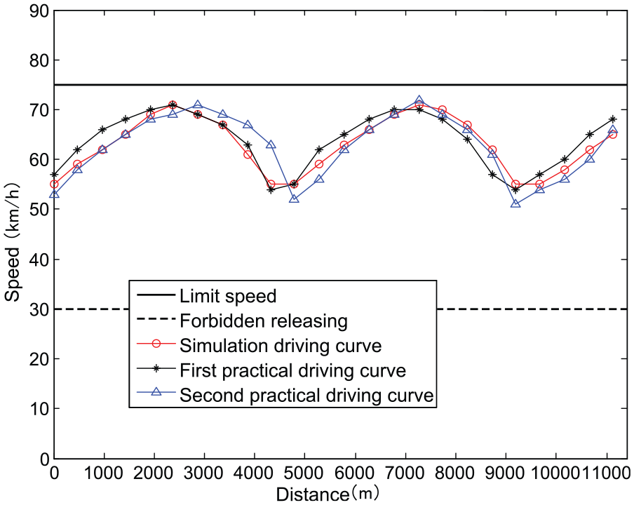
Simulation and practical HHT driving curves of scenario 2.
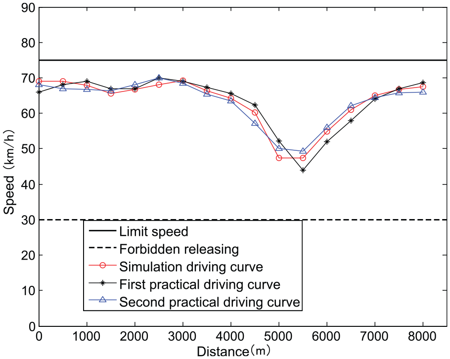
Simulation and practical HHT driving curves of scenario 3.
Simulation and practical HHT driving curves of scenario 4.
The corresponding data of Figures 11–14 are shown in Tables 8–11, respectively. The first column in the table denotes the running distance, the second column is the first practical speed of the train, and the third column is the second practical speed of the train. The fourth column denotes the simulation speed. The fifth column denotes twice the practical train BPR. The sixth column represents the train BPR in simulation. The FPDC and SPDC come from the driving data records of Shuohuang heavy-haul railway line, the value of the two curves are used to compare with the simulation results and to evaluate the effectiveness of method.
Simulation and practical driving curves data of scenario 1

BPR: braking pressure reduction.
Simulation and practical driving curves data of scenario 2.

BPR: braking pressure reduction.
Simulation and practical driving curves data of scenario 3.

BPR: braking pressure reduction.
Simulation and practical driving curves data of scenario 4.

BPR: braking pressure reduction.
In order to evaluate the simulation results, the authors define some evaluation indices, including average speed (AS), BD, expectation of speed difference between simulation curve and first practical curve (ESSF), and the corresponding variance between simulation and first practical curve (VSSF), the expectation and variance between simulation and second practical curve (ESSS/VSSS), the expectation and variance between first and second practical curve (ESFS/VSFS). According to the simulation results of four operation scenarios, evaluation indices are shown in Tables 12–15, respectively.
Simulation results of scenario 1.

AS: average speed; BD: braking distance; FPDC: first practical driving curve; SPDC: second practical driving curve; ESSF/VSSF: expectation and variance of speed difference between simulation curve and first practical curve; ESSS/VSSS: the expectation and variance between simulation and second practical curve; ESFS/VSFS: the expectation and variance between first and second practical curve; SDC: simulation driving curve.
Simulation results of scenario 2.
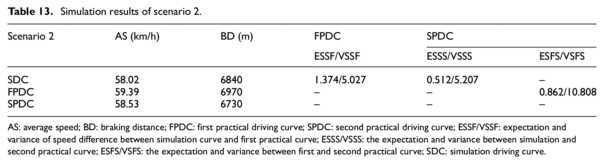
AS: average speed; BD: braking distance; FPDC: first practical driving curve; SPDC: second practical driving curve; ESSF/VSSF: expectation and variance of speed difference between simulation curve and first practical curve; ESSS/VSSS: the expectation and variance between simulation and second practical curve; ESFS/VSFS: the expectation and variance between first and second practical curve; SDC: simulation driving curve.
Simulation results of scenario 3.
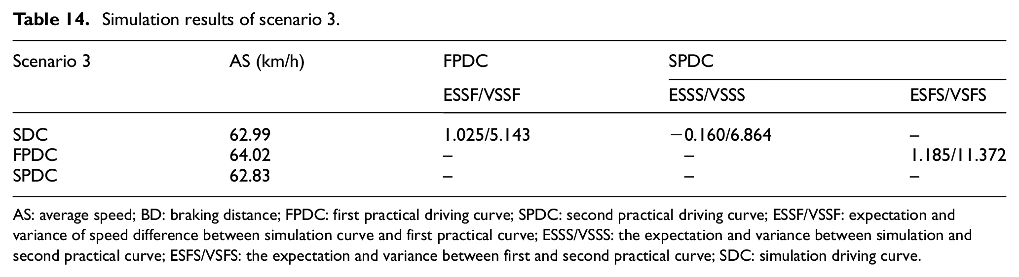
AS: average speed; BD: braking distance; FPDC: first practical driving curve; SPDC: second practical driving curve; ESSF/VSSF: expectation and variance of speed difference between simulation curve and first practical curve; ESSS/VSSS: the expectation and variance between simulation and second practical curve; ESFS/VSFS: the expectation and variance between first and second practical curve; SDC: simulation driving curve.
Simulation results of scenario 4.

AS: average speed; BD: braking distance; FPDC: first practical driving curve; SPDC: second practical driving curve; ESSF/VSSF: expectation and variance of speed difference between simulation curve and first practical curve; ESSS/VSSS: the expectation and variance between simulation and second practical curve; ESFS/VSFS: the expectation and variance between first and second practical curve; SDC: simulation driving curve.
Discussion
Based on the four typical operation scenarios of HHT, an NN driving curve generation method for HHT is proposed, which can be acted as a decision-support tool in this research. In the process, a different NN training algorithm is used and combined with the HHT characteristics and the braking operation model is built, the braking parameters are used in the motion equations and the simulation driving curves are achieved. Comparing simulation results with practical driving curves, the generation method is shown to be effective according to the speed, braking, and releasing actions of the corresponding curves, which have a similar target value for air BPR and operation trend.
The analysis of simulation results of four typical operation scenarios are as follows:
Scenario 1. A train stops at the station along a continuous downslope with initial downslope. The simulation results show that the AS differences between SDC and FPDC or SPDC are not more than ±1.73 km/h and the BD differences are not more than ±140 m. The ESSF and ESSS are 1.729 and −1.236, which are less than ESFS 2.965. The VSSF and VSSS are 18.543 and 4.38, which are all less than VSFS 32.424.
Scenario 2. A train stops at the station along a continuous downslope with initial upslope. The simulation results show that the AS differences between SDC and FPDC or SPDC are not more than ±1.37 km/h; the BD differences are not more than ±130 m. The ESSF and ESSS are 1.374 and 0.512, the ESSF is greater than ESFS 0.862, which means that speed difference between the simulation curve and the first curve is bigger than those between the first curve and the second curve, and the ESSS is less than ESFS. The VSSF and VSSS are 5.027 and 5.207, which are all less than VSFS of 10.808. The simulation results of scenario 1 and scenario 2 show that a train can run safely along a continuous downslope with initial slope and confirm that the method is effective.
Scenario 3. A train runs along a very steep slope with initial downslope. The simulation results show that the AS differences between SDC and FPDC or SPDC are not more than ±1.03 km/h. The ESSF and ESSS are 1.025 and −0.16, which are less than ESFS 1.185. The VSSF and VSSS are 5.143 and 6.864, which are all less than VSFS 11.372.
Scenario 4. A train runs along a very steep slope with initial flat slope. The simulation results show that the AS differences between SDC and FPDC or SPDC are not more than ±0.26 km/h. The ESSF and ESSS are 0.264 and 0.145, which are all greater than ESFS 0.119; the results show that speed differences between the simulation curve and the first curve, the simulation curve and the second curve are bigger than those between the first curve and the second curve. The VSSF and VSSS are 3.355 and 3.861, which are all less than VSFS 7.852. The simulation results of scenario 3 and scenario 4 show that a train can run safely under the maximum gradient of downslope with initial slope and confirm that the method is effective.
In order to get the train running curve, the rationality of running curve is judged by the limit speed value of different points of slope changing with the backing-off algorithm, when the calculated difference value between the train running speed and the limit speed exceeds the acceptable range, different backing-off strategies will be used to calculate the train running curve again, and the above process would be repeated until the calculated difference value meets the rationality. For the four kinds of HHT running scenarios in this article, there is no point of slope changing in the scenarios 1, 3, and 4; the rationality of driving curve cannot be judged by the limit speed changing; and the applicable conditions of backing-off algorithm cannot be met. And in the fourth step of NN algorithm proposed in chapter of the driving curve generating algorithm of the train, the conditions of limit speed changing and no limit speed changing conditions are both considered, the driving curve can be generated in the two conditions. So, the NN algorithm is not affected by the limit speed changing. Although the backing-off algorithm can be used in the scenario 2, it needs to iteratively calculate the difference value between the train practical speed and the limit speed in the point of slope changing and judging the rationality of driving curve simultaneously. The efficiency of entire process is low, which is generally suitable for offline calculation but not suitable for dynamic calculation. In comparison, the NN algorithm is intelligent and real-time dynamic calculation algorithm, which can be directly applied in engineering application.
The results of simulation and comparisons with back-off algorithm confirm the method of effectiveness and safety for generating a driving curve of an HHT. According to the modeling method of four typical scenarios, we can build more scenarios of the Shuohuang heavy-haul railway line and generate the driving curve of the whole line, which can be used to guide the driver’s driving operation as a decision-support tool.
For the different characteristics of heavy-haul lines and special operation scenarios, in the fourth step of NN algorithm proposed in chapter of the driving curve generating algorithm of the train, the curvature of the heavy-haul line should be considered to collect as a factor of training data. And some special operation scenarios, such as the auto-passing phase separation scenario, have effect on the driving curve generation, so how to improve the generalization ability of NN model should be considered. And, with the increase in the traction weight and the speed of the HHT, the driving curve is more closely related to the operation safety of the train. On one hand, more suitable modeling methods should be adopted to research the corresponding content to find more accurate driving curve, on the other hand, an automatic train driving method should be researched for a more efficient.
Conclusion
In this article, a driving curve generation method for HHTs based on NN model is proposed. Using the BP NN, the nonlinear braking operation model of an HHT is constructed. In the process of modeling, various nonlinear neurons are interconnected, and the field data are used to train the model. By taking the target value of train BPR as the controlled variable and then computing the train motion equation, the driving curve of an HHT using the NN model is generated finally. Based on four typical operation scenarios of HHT, four cases are conducted as examples, comparing simulation results with corresponding practical driving curves, the results show that the generation method is effective.
Footnotes
Academic Editor: Long Cheng
Declaration of conflicting interests
The author(s) declared no potential conflicts of interest with respect to the research, authorship, and/or publication of this article.
Funding
The author(s) disclosed receipt of the following financial support for the research, authorship, and/or publication of this article: This work was funded by the Beijing Jiaotong University basic scientific research funding projects under grant 2015JBM013, the Beijing municipal science and technology plan projects under grant D151100005815001, Shenhua Group scientific research funding projects under grant 20140269 and Beijing Laboratory for Urban Mass Transit.