Sage Journals: Discover world-class research

Abstract

The latest international survey shows that slow computational speed is still a significant issue for air brake models. Fluid dynamics air brake models can be more accurate but are slower in computing speed. Empirical models are reported as effective and more efficient. This article developed a new experimental based empirical air brake model that is more comprehensive and can be used to simulate both pneumatically and electronically controlled air brake systems, as well as locomotive air brake systems and brake systems for radio-based distributed power trains. Multiple functions were used to simulate various characteristics of brake cylinder pressures, which enables the model to capture more details. An activating algorithm was developed to further improve the computational efficiency. Case studies were conducted to compare the simulation results with experimental data. Simulation results and experimental data had good agreements regarding brake delays, force patterns and cylinder pressure amplitudes. The empirical air brake model is about 70 times faster than a fluid dynamics model and 7.4 times faster than real-time.

Keywords

Air brake modelling numerical simulation experimental data heavy haul train

Introduction

Railway air brakes are safety-critical systems for long heavy haul train operation. Though modelling of air brake systems has seen significant advancement in recent decades,¹ it remains as one of the most challenging steps for simulations of longitudinal train dynamics. A comprehensive international survey about air brake modelling was recently published in Wu et al.¹ According to this survey, air brake models can be roughly put into three groups. The first group was called fluid dynamics models; examples of such models can be found in Refs.^2–5 Fluid dynamics of brake pipes were considered and modelled by using partial differential equations that describe various governing laws: conservation of mass, momentum balance and energy balance. Flows and dynamics of the brake valves were then mainly described by modelling the air flows among various chambers, volumes and cylinders. Some lumped-parameter models^5,6 can also be regarded as fluid dynamic models. The second group of air brake models were called empirical models. Example of such models can be found in Refs.^7–12 Understandably, they did not explicitly model fluid dynamics behaviour of brake pipes and brake valves. Brake behaviour was simulated by fitting the time variations of pressure distributions among the studied brake cylinders. Various brake system characteristics were considered including maximum brake pressures, pressure changing rates and time delays. The third group of models were called fluid-empirical models. Such models can be found in Refs.^13–18 These models combined the features of the fluid dynamics models and empirical models by modelling brake pipes via fluid dynamics principles while modelling brake valves via the empirical way. Note that the difference between empirical air brake models (whole system models) and empirical brake valve model is that the inputs for the former are direct train driving commands from drivers, whereas the inputs for the latter are brake pipe pressures.

Computational speed is a major issue for simulations relative studies of long heavy haul trains due to the complicity of modelling and large number of vehicles.¹⁹ The international survey¹ has also pointed out the computational speed issue of air brake modelling as one of the ongoing research topics. The fluid dynamic methodology for air brake system modelling requires solving partial differential equations, which is more complex than other parts of longitudinal train dynamics, such as modelling of tractive and dynamic brake forces, modelling of resistance forces. Therefore, fluid dynamic air brake models can be a primary contributor for the slow computational speed issue. Note that the significance of computational speed also depends on the scale of the problem analysed. For simulations where only small number of vehicles and/or short simulated time is required, the computational speed becomes relatively insignificant, as the total simulation time should be acceptable anyway. Whereas for simulations that do require simulations of many vehicles and long simulated time, such as whole-trip simulations and optimisation studies,^20–22 computational speed becomes significant. Fast air brake models are also chased by researchers who focus on train driving controls.^23,24 Empirical models have been reported as computationally efficient as well as effective.^6–12 For longitudinal train dynamics simulations, results required from air brake system models are brake forces, therefore brake pipe models are not required, which also makes empirical models justified. In addition, modern intelligent transport systems often require fast models to predict system performance and to adjust train control actions. Fast empirical air brake models can play some roles in these systems as well.

This paper presents a new empirical air brake model that is developed from experimental data. Compared to other empirical air brake models, the new one has integrated a signal source searching algorithm to enable the simulations of radio-based DP trains. Multiple functions are used to simulate the time history of brake cylinder pressures, which enables the model to simulate more details. The new model can simulate multiple types of air brake systems including Pneumatically Controlled Pneumatic (PCP) brake system or Pneumatically Controlled Air brake system, Electronically Controlled Pneumatic (ECP) brake systems and locomotive air brake systems.

Air brake systems and experimental data

In this section, the working mechanism of PCP brake systems will be briefly discussed; and then experimental data about PCP brake systems, ECP brake systems, radio-based Distributed Power (DP) control and locomotive air brake systems will be presented.

Air brake systems

Railway trains have used various types of air brake systems at different development stages. These include direct air brake systems²⁵ that are not used in modern railway operation anymore; vacuum brake systems²⁶ that were mainly seen on Indian railways; and the most widely used automatic air brake systems.¹ Automatic air brake systems are the most widely used systems and they have become a norm for long heavy haul trains. Brake related issues, such as brake delays, have been a major limitation for the development of long heavy haul trains. In recent decades, two technologies have significantly reduced the limitation and have promoted the development of heavy haul trains; they are cable-based ECP and radio-based DP control (e.g. the Locotrol technology).²⁷ Note that in this article, ECP refers to cable based ECP, and PCP refers to the automatic PCP systems.

As shown in Figure 1, a railway train air brake system usually includes sub-systems for locomotives and waggons. Driver’s control valve is commonly located on the first locomotive. It is noted that the locomotive brake system in Figure 1 is heavily simplified; more information of actual locomotive brake systems can be found in Specchia et al.⁴ Once a brake command is applied from the driver’s brake valve, the system starts to discharge air from the brake pipe to atmosphere so as to reduce air pressures of the brake pipe. The pressure reduction transmits from the lead locomotive to the tail of the train along the brake pipe. This pressure reduction causes a lower pressure compared with waggon auxiliary reservoirs. If the pressure difference between bake pipe and auxiliary is significant enough, or the pressure reduction rate in the brake pipe is significant enough, the waggon brake valve will apply brake by connecting waggon auxiliary reservoir and brake cylinders. On the contrary, once a release command is applied from the driver’s valve, brake pipe will stop discharging air to atmosphere and pressurised air will be charged from the main reservoir to brake pipe so as to bring the brake pipe pressure back to its rated level. Similarly, this pressure increase will also transmit from the lead locomotive to the tail of the train. Once the pressure difference between the brake pipe and waggon auxiliary reservoir is small enough, waggon brake valve will switch the connection of brake cylinder from auxiliary reservoir to atmosphere to release brake cylinder. Above is a brief description of the brake and release processes of air brake systems, more details about different features of different air brake systems can be found in Wu et al.¹

Figure 1.

PCP brake system.

Brake delay is an important issue for modelling of air brake system. The pattern of brake delay for head-end trains is straightforward: waggons brake one by one from the head to the tail of the train. For trains with radio-based DP control, the brake delay is shown as Figure 2. Assume that there are three locomotives in the DP train; and Loco 1 is the master locomotive as shown in Figure 2(a). The master locomotive sends out brake signals to slave locomotives, that is, Loco 2 and Loco 3. Radio signals usually take seconds to be received and processed by slave locomotives. Figure 3 illustrates some test results about the delays for slave locomotives to response to the control signals of the master locomotive.²⁷ From the test results, it can be seen that there is about 50% of possibility that slave locomotives will take about 3 s to response. Therefore, before slave locomotives response to the brake signals, waggons that close to the master locomotive have started braking, as shown in Figure 2(b). To be able to model the air brake system, it is assumed that locomotives are the sources of brake signals; and for each waggon, there is only one signal source, that is, the one whose signal reaches the waggon first. In Figure 2, waggons numbered as ‘0’ are not braking; and those numbered as ‘1’, ‘2’ or ‘3’ are. Meanwhile, the numbers can be regarded as the signal sources of waggons. Combining the implications of radio signal propagation and that of brake wave propagation, a status shown as Figure 2(c) will be reached.

Figure 2.

Brake delay in trains with radio-based DP control: (a) start of the process, (b) signals reach remote locomotives and (c) brake pressure changes propagation.

Figure 3.

Radio-based DP control performance.

ECP systems use on-board cables to transmit brake signals as shown in Figure 4. Since air pressure signals and radio signals are replaced by electronic signals, there is almost no brake delay for waggons in the trains; brake applications throughout the train are applied at almost the same time.

Figure 4.

Train with the ECP system.

Experimental data

Brief information of the experimental data used in this paper is listed in Table 1. All data about the type 120 brake valve were provided by Southwest Jiaotong University, China, they were measured on an indoor test rig that had the capability of simulating 150 brake valves at a time. The left column of Figure 5 is a representation of the dataset 1 in Table 1. The experimental data is plotted side-by-side with simulated results from Section 4. In this figure, the numbers in the legends indicate the position of the waggon brake valve in the train. It is noted that in Figure 5(c), (e) and (g), the brake release data is not available. This is also mainly due to the fact that brake cases of 140 kPa, 170 kPa, and the emergency are mainly used to stop the train and when the train is stopped, the brake release performance is less significant than that in the 50 kPa case which is usually used to correct train speeds during normal operation.

Table 1.

Descriptions of experimental data.

Data	Brake system	Valve number	Measured scenarios	Measured positions
Set 1	Chinese type 120 valve	150	50 kPa+release, 140 kPa, 170 kPa and Emergency	1st, 75th and 150th
Set 2	Chinese type 120 valve	150	50 kPa+release, 140 kPa and emergency	1st, 75th and 150th
Set 3	Chinese type 120 valve	120	50 kPa+release, 70 kPa+release, 100 kPa+release, 170 kPa+release and Emergency	1st and 120th
Set 4	Chinese type 120 valve	108	50 kPa+release, 70 kPa+release 170 kPa+release	Every 10 waggon
Set 5	Chinese ECP	7	170 kPa+release	All
Set 6	Imported ECP	150	Full-service brake	1st, 75th and 150th
Set 7	Chinese HXD locomotive	2	50 kPa+release, 150 kPa+release and emergency	All
Set 8	Chinese HXD locomotive	2	50 kPa+release and 150 kPa+release	All

Figure 5.

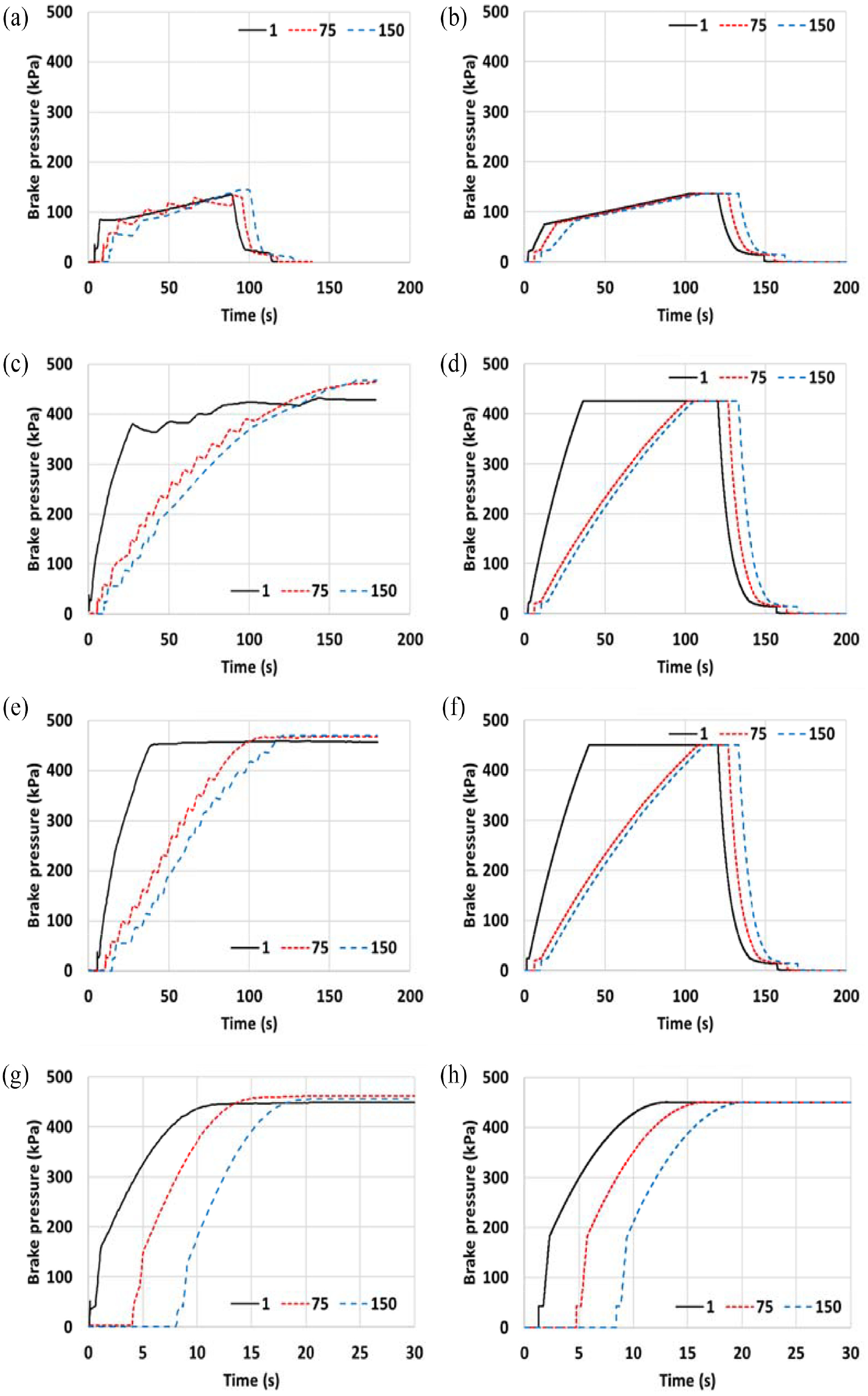
Brake cylinder pressure results of a PCP system (the pressure in sub-captions indicate final pressure reduction of the brake pipe): (a) measured results, 50 kPa, (b) simulated results, 50 kPa, (c) measured results, 140 kPa, (d) simulated results, 140 kPa, (e) measured results, 170 kPa, (f) simulated results, 170 kPa, (g) measured results, emergency and (h) simulated results, emergency.

Two sets of experimental data (dataset 5 and dataset 6 in Table 1) about ECP systems²⁸ were used. The measured results in Figure 6(a) are representations of the dataset 5. Note that since the brake cylinder pressures at different positions overlap each other in the time domain, only one curve was plotted in Figure 6.

Figure 6.

Results of an ECP system: (a) measured results and (b) simulated results.

Two sets of experimental data (datasets 7 and 8) about locomotive air brake systems were provided by Southwest Jiaotong University, China. Datasets 7 and 8 were measured on a test bench for air brake systems used on Chinese HXD electric locomotives. Figure 7(a) is a representation of dataset 7. In the figure legends, 50 and 150 kPa indicate brake commands with 50 and 150 kPa (brake pipe) pressure reductions respectively.

Figure 7.

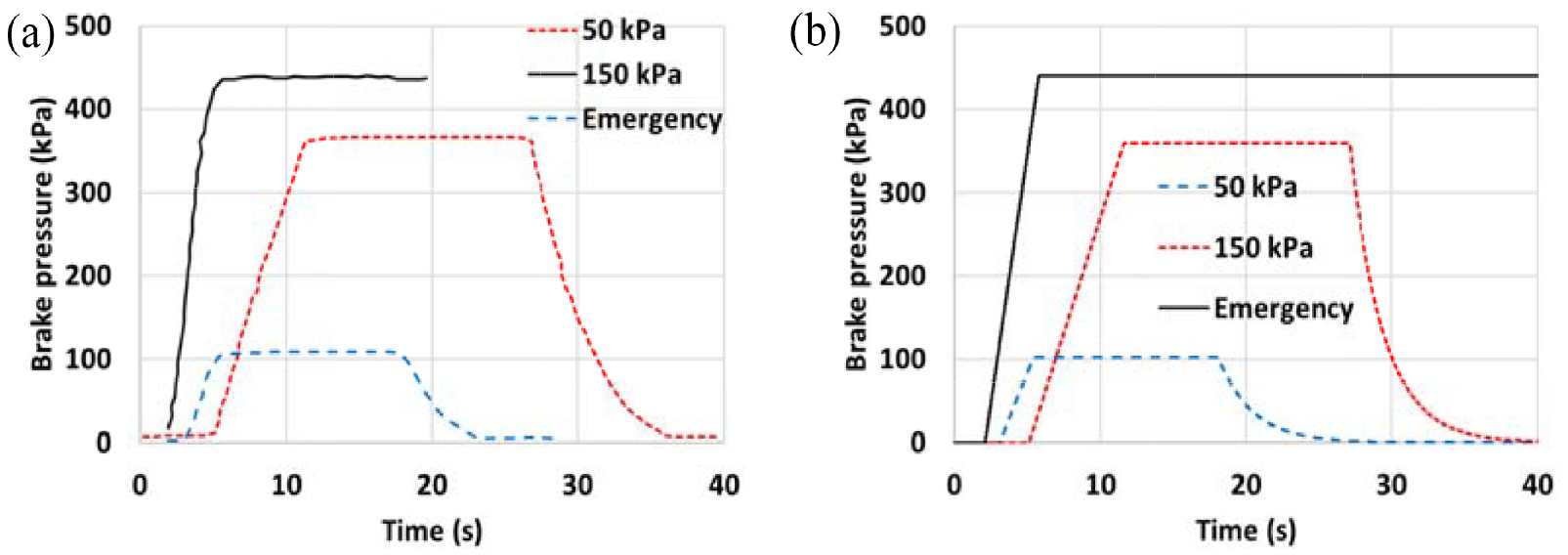
Results of locomotive air brake system: (a) measured results and (b) simulated results.

Modelling of air brake

Modelling will first focus on PCP systems, and then models of ECP systems and locomotive air brake systems can be easily derived from that of PCP systems. To develop an empirical air brake model, the first step is to characterise the dynamic behaviour of the air brake system and to determine their quantifying parameters. Then, a mathematic function has to be selected to fit quantifying parameters. During this process, fitting tools such as the Matlab can be used.

Brake pressures in steady states

Brake cylinder pressures after an air brake system reaches a steady state (e.g. pressure after the 20th second in Figure 5(g)) is considered as a nonlinear function of the inputs, that is, the brake commands indicate the final pressure reductions in the brake pipe,

P_{s} = ε f_{1} (P_{r}),

(1)

where $P_{r}$ is brake commands that indicate the final pressure reduction; $P_{s}$ is the brake cylinder pressures in a steady state; $ε$ is a parameter used to account for empty-load or diaphragm type brake system, that is, load dependent pressure control; $f_{1}$ is a look-up table function. Note that in some books, such as Rao,²⁵ linear function expressed as equation (2), is used.

P_{s} = P_{r} V_{a} / V_{b} - 100,

(2)

where $V_{a}$ is the volume of the auxiliary reservoir; $V_{b}$ is the volume of the brake cylinder. Whereas information abstracted from experimental data indicates that a nonlinear function is required.

Brake delay

Time delays of brake and release of air brakes are influenced by the propagation speeds of pressure waves in brake pipes as well as by the formations of different trains, that is, positions of the locomotives and number of waggons. In this paper, pressure wave propagation speed is modelled as a nonlinear function of the brake inputs as:

v_{air} = f_{2} (P_{r}),

(3)

where $v_{air}$ is pressure change wave propagation speed; $f_{2}$ is a look-up table function. To determine brake delays for waggons in a DP train, their signal sources have to be determined as discussed in Section 2.1. An algorithm expressed as equation (4) can be used to determine the time delay for waggons.

t_{d, i} = \min {t_{dL, j} + \frac{s_{i} - s_{L, j}}{v_{air}}} (j = 1, n_{loco}),

(4)

where $i$ indicates the waggon position in the train; $t_{d, i}$ indicates the time delay experienced by the $i^{th}$ waggon; $j$ indicates the sequence number of the locomotive; $n_{loco}$ indicates the number of locomotives that are being used in the train; $t_{dL, j}$ is the time delay of the radio signal received by the $j^{th}$ locomotive; $s_{i}$ is the waggon position in meterage on the track of the $i^{th}$ waggon; $s_{L, j}$ is the position in meterage on the track of the $j^{th}$ locomotive. Since the nearest signal source for a locomotive is the locomotive itself, $(s_{i} - s_{L, j})$ will be zero for locomotives, which means equation (4) can be used for all vehicles in the train, including waggons and locomotives. Note that for trains that are equipped with end-of-train (EOT) devices²⁷ or so-called train tails, the last waggon has to be taken as a signal source.

Brake cylinder charging

As can be seen from the measured data in Figure 5, the charging processes for brake cylinders are of nonlinearity in the time domain. And the charging processes for cylinders at different positions are different from each other. A summary of various braking scenarios can lead to that the overall pattern of the charging processes is of an approximate exponential pattern; therefore, an equation expressed as equation (5) was proposed to approximate the processes.

\begin{matrix} P_{i, t} = P_{m, i} + (P_{s} - P_{m, i}) {1 - \exp [- β_{i} (t - t_{d, i})]} \\ (P_{s} \leq P_{i, t} \leq P_{m, i}), \end{matrix}

(5)

where $t$ indicates time; $P_{i, t}$ indicates the current brake pressure on the $i^{th}$ waggon of the train; $P_{m, i}$ indicates the most recently changed brake cylinder pressure. $β_{i}$ is a parameter that is used to adjust pressure ascending rate, this control parameter is further modelled as:

β_{i} = f_{3} (P_{r}, k_{i}) γ_{i},

(6)

$k_{i}$ indicates the number of waggons that are located between the studied waggon and its nearest locomotives; $γ_{i}$ is parameter that is used to further adjust the charging parameter ( $β_{i}$ ) for the purpose of modelling DP trains; $f_{3}$ is a three-dimensional look-up table function in which pressure reduction and waggon position are used as searching interpolating indexes. Note that there can be two types of signal sources in a train, that is, locomotive and EOT device. Therefore, a waggon can be located between three types of signal source combinations: locomotive-locomotive (e.g. in the first waggon group of a DP train), locomotive-EOT (e.g. in the last waggon group of a train with an EOT device) and locomotive only (e.g. in a head-end train without EOT devices). Experimental data indicates that the changing patterns of charging rates along the train for different combinations are different; therefore, $γ_{i}$ shall have different values according to signal combinations.

As can be seen from Figure 5 that the nonlinearities of the charging processes include other characteristics, for example, the surging of pressure at the very beginning of the brake application; rapid linear increase in the emergency brake scenario (e.g. 2nd–3rd second of the waggon 001, Figure 5(g)) and the slow increase in the minimum brake scenarios (20th–80th second of the waggon 001, Figure 5(a)). All these characteristics can be simulated by using extra correction functions, as shown in Figure 8, to confine brake pressures within certain ranges.

Figure 8.

Correction functions.

Modelling of brake cylinder release

Release models are similar to that for brake cylinder charging, which are expressed by exponential function (equation (7)) and correction functions.

P_{i, t} = P_{s} + (P_{m, i} - P_{s}) \exp [- δ_{i} (t - t_{d, i})] (P_{s} \leq P_{i, t} \leq P_{m, i}),

(7)

where $δ_{i}$ is a similar parameter to $β_{i}$ , which is used to modify the releasing rate. Summary of experimental data leads to the expression of equation (8).

δ_{i} = f_{4} (P_{r}) φ_{i},

(8)

where $φ_{i}$ is a similar parameter to $γ_{i}$ , which is used to modify $δ_{i}$ for DP trains; $f_{4}$ is a look-up table function used to for $δ_{i}$ .

Modelling of ECP and locomotive air brake

Modelling of ECP is based on the PCP model described in Sections 3.1–3.4. To derive an ECP model, differences between PCP and ECP systems have to be acknowledged. First, ECP uses on-board cable instead of air brake waves to transmit control signals. Therefore, the signal speed for ECP is significantly faster than that of PCP systems. For ECP models, equation (3) can be replaced by a relatively big constant value (e.g. 3000.0); and $t_{dL, j}$ in equation (4) can be replaced by a small constant value (e.g. 0.01). By doing so, source codes for PCP brake models can be used with minor changes, so it will be easy to switch between ECP systems and PCP systems for different simulations. As the charging rate and release rate for ECP systems are generally higher than that of PCP systems (twice the rates of PCP emergency case), certain adjustments for parameters in equations (6) and (8) are needed.

For locomotive air brake models, delays of radio signals have to be considered; this can be done by using the algorithm expressed by equation (4). Locomotive air brake systems are usually direct brake systems, by examining the experimental data shown as Figure 7(a) it can be found that the charging process can be approximated as linear. While the slopes for charging processes are related to brake signals. Another nonlinear function, $f_{5}$ (equation (9)), has to be developed to fit the relationship between brake signals and slopes.

k_{c} = f_{5} (P_{r}),

(9)

where $k_{c}$ is the charging slope. In regard to the modelling of release for locomotive air brake, equation (7) can still be used but with different parameters. A set of example parameters used for the look-up table functions are listed in Table 2. It is noted that the parameters can only be used for the results presented in Figures 5 and 7.

Table 2.

Key parameters for look-up table functions.

Function (unit)	50 kPa	70 kPa	100 kPa	140 kPa	170 kPa
$f_{1}$ (kPa)	137	250	340	452	464
$f_{2}$ (m/s)	220	220	220	220	220
$f_{3}$ before 120th (-)	2.52e-2	2.45e-2	2.30e-2	2.05e-2	1.83e-2
$f_{3}$ after 120th (-)	1.52e-2	1.20e-2	0.90e-2	0.73e-2	0.68e-2
$f_{4}$ (-)	0.150	0.156	0.162	0.170	0.180
$f_{5}$ (-)	54.50	59.22	61.75	62.00	62.00

A comparison of the measured and simulated pressure ascending time of the results presented in Figures 5 to 7 is summarised in Table 3. It is noted that in the modelling method presented in this paper, maximum steady brake cylinder pressures and brake delays directly uses the parameters summarised from the measured results, therefore there is no differences in these two parameters. Under this simulation, the ascending time is compared as recommended in Wu et al.¹ In this table the difference is calculated as (Simulated-Measured)/Measured and is presented in percentages. For the PCP case, only results of the waggon 150 are presented as simulation experience indicates that waggon 150 usually shows the largest differences between the simulation and measured results. The results show that stimulation results were well matched with experimental data; the maximum difference between the measured and simulated results was less than 10%.

Table 3.

A comparison of the pressure ascending time.

Case	Measured (s)	Simulated (s)	Difference (%)
PCP 50 kPa waggon 150	92.03	98.40	7
PCP 140 kPa waggon 150	104.06	98.25	−6
PCP 170 kPa waggon 150	109.48	104.66	−4
PCP Emergency waggon 150	11.20	11.60	4
ECP	5.42	5.04	−7
Locomotive 50 kPa	2.41	2.60	8
Locomotive 150 kPa	6.49	6.55	1
Locomotive emergency	3.36	3.66	9

Further improvement of computational speed

Simulation experience indicates that for whole-trip simulations brake applications take account of a very small portion of the total simulated time. For example, for a whole-trip simulation that lasts for 3 h (simulated time), brake applications could only take 20 min (simulated time). For conventional longitudinal train dynamics simulations, air brake forces are computed for every time-step. It is understandable that there is no brake force if brake applications are not applied or the brake release command has been issued for a while, for example, 120 s after the brake release command. In other words, for a large portion of simulated time, brake forces do not have to be computed. Combing the fact that air brake models (especially fluid dynamic models) are relatively computationally expensive, significant amount of computing time can be saved from the conventional scheme of air brake models.

In this article, an algorithm shown as Figure 9 and expressed as equation (10) was developed to activate computing of air brake forces when it is necessary.

{\begin{matrix} P_{s} > 0 & activated \\ P_{s} = 0 . and . t_{m} > 120 & deactivated \end{matrix}

(10)

Figure 9.

Activation of air brake model.

where $t_{m}$ is the most recent time when the brake signal was changed. Numerical experiments indicate that for the programme used in this article, about 20% of simulation time can be reduced (whole-trip simulations, 214 vehicles, no shorter than 1 h of simulated time) by adding the algorithm expressed as equation (10).

Case studies

Simulations were carried out against experimental data for PCP systems, ECP systems and locomotive brake systems. Corresponding simulated results have been plotted in Figures 5, 7 and 8. Note that simulation conditions for these results were the same with corresponding experimental conditions. Simulation results show that the empirical air brake model developed in this paper is well matched with experimental data regarding various system behaviour, for example, brake delays, pressure amplitudes and force patterns.

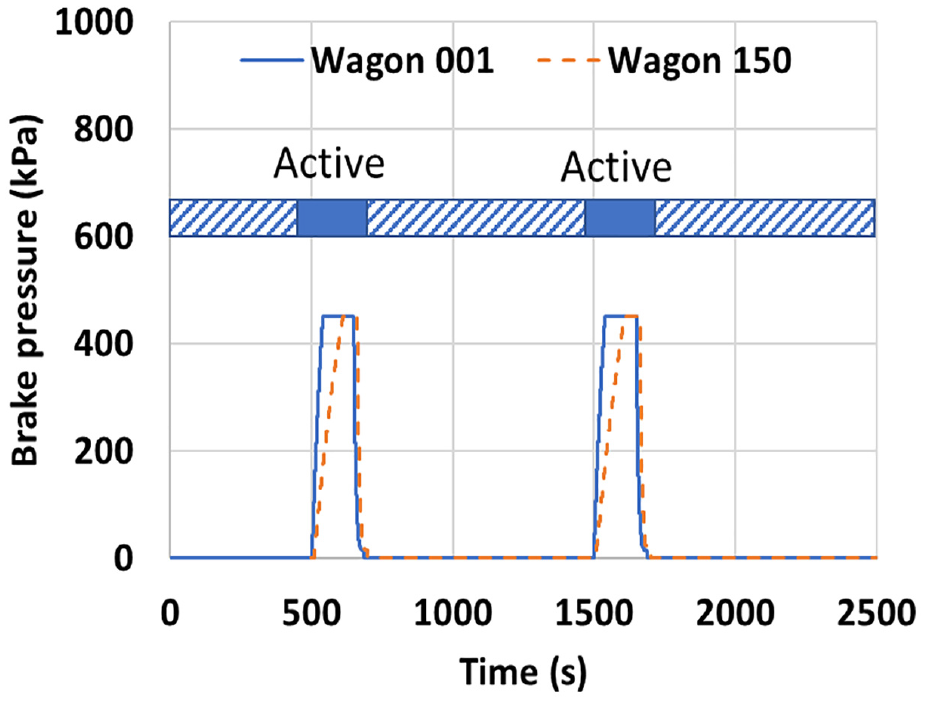
To examine the patterns of brake delays for DP trains, a long heavy haul train model was developed to use two locomotives at the front and then 105 waggons, and then two locomotives in the middle and then 105 waggons at the end. Emergency brakes for DP trains with and without EOT devices were simulated. Delays of radio signals for all slave locomotives and EOT devices were 3.5 s; the corresponding simulated results are shown as Figure 10. As can be seen form Figure 10, the simulated patterns of brake delays agree with the discussions in Section 2.1.

Figure 10.

Simulated results of radio-based DP trains: (a) with EOT devices and (b) without EOT devices.

To demonstrate the advantage of the empirical model in terms of computational speed, the same simulations presented in Figure 10 were repeated using the fluid dynamics model developed in Wu et al.²⁹ The computing time of the simulations is compared in Table 4. The results show that the detailed fluid dynamics model was about 9.5 times slower than real-time. To simulate a 25-s brake operation, the fluid dynamics model required about 240 s. However, the empirical air brake model was significantly faster. The same simulations only took the empirical model 3.4 s, which was about 7.4 times faster than real-time. comparatively, the empirical model was about 70 times faster than the fluid dynamics model.

Table 4.

Summary of computing time.

Simulation cases	Brake operation time (s)	Computing time (s)
Simulation cases	Brake operation time (s)	Fluid dynamics model	Empirical model
With EOT devices	25	242	3.4
Without EOT devices	25	238	3.4

Discussion and conclusion

The latest survey¹ shows that slow computational speed is still a significant issue for air brake models. Fluid dynamic models can be more accurate to simulate air brake systems; empirical models have their own advantages, specifically, sufficiently accurate, effective and more computationally efficient. For large scale long heavy haul train simulations, empirical models can be a good choice. The limitation for empirical models is that a final model can be limited to the formation of the train and the specific type of the brake system from which the experimental data were obtained from. For the empirical model to be used for a different train formation and a different type of air brake system, model equations proposed in this paper can be used but the specific model parameters may need to be adjusted. For the development of a comprehensive model, all commonly seen brake and release cases are recommended to be considered during the model development process.

Compared to other empirical models, the model developed in this article is more comprehensive, which can be used to simulate PCP, ECP and locomotive air brake systems. It can also be used to simulate radio-based DP trains. A special algorithm to further improve the computational efficiency of the new model was developed. Numerical experiments indicate that about 20% of improvement for computational efficiency can be achieved for whole-trip simulations. Experimental data about PCP brake systems, ECP brake systems, radio-based DP control and locomotive air brake system were presented. Simulation results were well matched with experimental data regarding time delays, pressure patterns and cylinder pressure amplitudes. Computational speed of the empirical air brake model was compared with a fluid dynamics air brake model. The results show that the empirical air brake model is about 70 times faster than the fluid dynamics model and 7.4 times faster than real-time.

Footnotes

Handling Editor: Chenhui Liang

Declaration of conflicting interests

The author(s) declared no potential conflicts of interest with respect to the research, authorship, and/or publication of this article.

Funding

The author(s) received no financial support for the research, authorship, and/or publication of this article.

ORCID iD

Honghua Wu

References

Cole

Spiryagin

, et al. Freight train air brake models. Int J Rail Transp. Epub ahead of print 21 December 2021. DOI: 10.1080/23248378.2021.2006808.

Wei

, et al. An air brake model for longitudinal train dynamics studies. Veh Syst Dyn 2017; 55: 517–533.

Pugi

Rindi

Ercole

, et al. Preliminary studies concerning the application of different braking arrangements on Italian freight trains. Veh Syst Dyn 2011; 49: 1339–1365.

Specchia

Afshari

Shabana

, et al. A train air brake force model: locomotive automatic brake valve and brake pipe flow formulations. Proc IMechE, Part F: J Rail and Rapid Transit 2013; 227: 19–37.

Teodoro

ÍP

Eckert

Lopes

, et al. Parallel simulation of railway pneumatic brake using OpenMP. Int J Rail Transp 2020; 8: 180–194.

Kamiński

. A simplified lumped parameter model for pneumatic tubes. Math Comput Model Dyn Syst 2017; 23: 523–535.

Nasr

Mohammadi

. The effects of train brake delay time on in-train forces. Proc IMechE, Part F: J Rail and Rapid Transit 2010; 224: 523–534.

Murtaza

. Railway air brake simulation: an empirical approach. Proc IMechE, Part F: J Rail and Rapid Transit 1993; 207: 51–56.

Luo

Cole

. Longitudinal dynamics and energy analysis for heavy haul trains. J Mod Transp 2014; 22: 127–136.

10.

Oprea

Cruceanu

Spiroiu

. Alternative friction models for braking train dynamics. Veh Syst Dyn 2013; 51: 460–480.

11.

Wang

Tang

. Optimal control of heavy haul train based on approximate dynamic programming. Adv Mech Eng 2017; 9: 1–15.

12.

Huang

Bai

Meng

, et al. Research on the driving strategy of heavy-haul train based on improved genetic algorithm. Adv Mech Eng 2018; 10: 1–16.

13.

Belforte

Cheli

Diana

, et al. Numerical and experimental approach for the evaluation of severe longitudinal dynamics of heavy freight trains. Veh Syst Dyn 2008; 46: 937–955.

14.

Cantone

Crescentini

Verzicco

, et al. A numerical model for the analysis of unsteady train braking and releasing manoeuvres. Proc IMechE, Part F: J Rail and Rapid Transit 2009; 223: 305–317.

15.

Cantone

Durand

. Longitudinal forces evaluation of SNCF trains. Paper presented at: the 9th World Congress on Railway Research, Lille, France, 22–26 May 2011.

16.

Schick . A digital test bench for pneumatic brakes simulating the brake behaviour of freight trins. Master’s Thesis, KTH Sweden, 2021.

17.

Abdol-Hamid

. Analysis and simulation of the pneumatic braking system of freight train. PhD Thesis, University of New Hampshire, 1986.

18.

Cantone

. TrainDy: the new Union Internationale Des Chemins de Fer software for freight train interoperability. Proc IMechE, Part F: J Rail and Rapid Transit 2011; 225: 57–70.

19.

Evans

Berg

. Challenges in simulation of rail vehicle dynamics. Veh Syst Dyn 2009; 47: 1023–1048.

20.

Bosomworth

Spiryagin

Alahakoon

, et al. The influence of vehicle system dynamics on rail foot heat transfer. Aust J Mech Eng 2018; 16: 126–138.

21.

McClanachan

Cole

. Current train control optimization methods with a view for application in heavy haul railways. Proc IMechE, Part F: J Rail and Rapid Transit 2012; 226: 36–47.

22.

Cole

Spiryagin

. Parallel computing enables whole-trip train dynamics optimizations. J Comput Nonlinear Dyn 2016; 11: article no. 044503.

23.

Huang

Tan

Chen

, et al. A neural network driving curve generation method for the heavy-haul train. Adv Mech Eng 2016; 8: 1–14.

24.

Huang

Zhang

Guo

, et al. Synchronous control system based on wireless data transmission for 50,000-t heavy-haul trains. Adv Mech Eng 2018; 10: 1–9.

25.

Rao

. Train brake. 2nd ed. Beijing: China Science Publishing House, 2010. (in Chinese)

26.

Bharath

Nakra

Gupta

. Modelling and analysis of pneumatic railway brake system. Appl Math Model 1990; 14: 58–66.

27.

Geng

. Heavy-haul transportation technologies on Datong-Qinhuangdao Railway. Beijing: China Railway Publishing House, 2010 (in Chinese).

28.

Zhang

. Test and simulation study on traction and brake system of combined heavy haul train. PhD Thesis, China Academy of Railway Sciences, Beijing, China 2009. (in Chinese)

29.

Cole

Spiryagin

, et al. Railway air brake model and parallel computing scheme. J Comput Nonlinear Dyn 2017; 12: article no. 051017.

An experiment-based empirical model for heavy-haul train air brake

Abstract

Keywords

Introduction

Air brake systems and experimental data

Air brake systems

Experimental data

Modelling of air brake

Brake pressures in steady states

Brake delay

Brake cylinder charging

Modelling of brake cylinder release

Modelling of ECP and locomotive air brake

Further improvement of computational speed

Case studies

Discussion and conclusion

Footnotes

Declaration of conflicting interests

Funding

ORCID iD

References