Stability analysis of machine tool spindle under uncertainty

Abstract

Chatter is a harmful machining vibration that occurs between the workpiece and the cutting tool, usually resulting in irregular flaw streaks on the finished surface and severe tool wear. Stability lobe diagrams could predict chatter by providing graphical representations of the stable combinations of the axial depth of the cut and spindle speed. In this article, the analytical model of a spindle system is constructed, including a Timoshenko beam rotating shaft model and double sets of angular contact ball bearings with 5 degrees of freedom. Then, the stability lobe diagram of the model is developed according to its dynamic properties. The Monte Carlo method is applied to analyse the bearing preload influence on the system stability with uncertainty taken into account.

Introduction

The dynamics of spindle system plays a crucial role in machining processes. During the process, vibrations between the workpiece and the cutting tool may cause degradations of machining accuracy and surface processing quality. The vibrations are usually classified into two types according to their sources: forced vibrations induced by periodic varying cutting loads and self-excited chatter vibrations caused by the variation in chips thickness, which is the result of dynamic cutting forces and in turn modulates the cutting force. ¹ Combined with the effects of these vibrations, if the spindle-tool-workpiece system works in unstable state, the cutting force may grow very large until the tool cracks. The forced cutting vibrations cannot be eliminated but can be reduced to an accepted level with respect to both costs and technical feasibility. It is well known that the onset of chatter is bound up with the process parameters, such as spindle speed, depth of cut;^2,3 therefore, by keeping these parameters below certain limits, unstable cutting vibrations can be avoided.

The foundation of chatter theory and study on the stability of the cutting process is ascribed to Tlusty and Tobias. Then, a considerable amount of research related to selection of chatter-free process parameters has been done for decades. In order to determine the boundaries of stable machining with high material removal rates, the dynamic property of the spindle-tool system is required in terms of the tool nose frequency response function (FRF). It can be obtained analytically or experimentally. The experimental approaches involve modal testing techniques. However, the testing is time-consuming and has to be repeated for different machines. And even when a minor adjustment is made to the spindle-tool assembly, a new test will be needed since the spindle-tool system dynamics has changed. Schmitz and colleagues^4,5 and Erturk et al. ⁶ implemented receptance coupling theory of substructures dynamics in order to reduce the number of tests. The main idea underlying their proposals can be summarized as follows: first, investigating the dynamical properties of different specifications of the components of spindle-tool assembly individually, such as spindles, toolholder and tools, instead of the dynamics of a specific spindle–toolholder–tool combination as a whole; then, determining the coupling parameters between the components’ contact interface, such as cross FRF stiffness and damping ratio; and finally, the dynamics of components concerned are combined as desired to obtain the dynamics of a specific spindle–toolholder–tool assembly. The first two steps can be done analytically or experimentally, while the last step almost offline analytically.

However, in a real machining situation, there are usually some uncertainties that make the dynamic performance of a spindle system not as consistent with the experimental and analytical hybrid model as expected. Even the same model of spindles may exhibit different dynamic performance because of the variations of commissioning conditions, for example, the preload of bearings during spindle installation. The Monte Carlo simulation is an effective approach to address uncertainty in engineering analysis, provided that the uncertainty factors could be described as random variables with certain statistical distributions.^7,8

The purpose of this article is to perform a Monte Carlo–based study to investigate the stability predictions of the spindle systems under uncertainty. Specifically, a spindle system is first constructed using the finite element method with Timoshenko beam elements to idealize its shaft including the tool, and the bearings are idealized by two 5 degree-of-freedom (DOF) stiffness models. In the modelling, the system’s structural damping coefficients and bearings preload are assumed to be random variables to simulate uncertainty effects. Subsequently, the dynamics of the analytical spindle system model is computed with Monte Carlo simulation. Then, the system’s stability lobe diagrams are generated and the reliability of the stability boundary is analysed.

Dynamics model of spindle systems

Figure 1(a) shows the spindle assembly of a high-speed milling centre. The shaft is supported by two groups of HSS71922 angular contact ball bearings in tandem at the front and the rear, respectively, and is designed to operate up to 12,000 r/min with a 20 kW motor connected to the shaft with a reducer.

Figure 1.

Spindle system: (a) physical prototype and (b) finite element model scheme.

In this article, the methods for the modelling of spindle systems presented by Nelson ⁹ and Cao and Altintas ¹⁰ were applied with some simplifications. Since the main purpose is not a repetition of comprehensively modelling the spindle system but an application of its dynamics information to predict the stability with reliability, the contact interfaces of the toolholder and the holder-shaft are assumed to be rigid. The finite element model of the spindle system is shown in Figure 1(b). The black dots represent element nodes, and the white circles represent the nonlinear spring models for the bearings.

Modelling of the shaft

A typical two-node Timoshenko beam element is shown in Figure 2, with a Cartesian reference coordinate system, X-Y-Z. Every node of the element has 5 DOF: three translational u, v and w with respect to the X-, Y- and Z-axes, respectively, and two rotational degrees Ω _y and Ω _z with respect to the Y- and Z-axes. The dashed line between nodes 1 and 2 is the longitudinal axis of the beam.

Figure 2.

Timoshenko beam.

Therefore, the inertia matrix M^e of an element is a 10-dimension symmetric matrix and can be expressed as follows

$$\begin{array}{cc}\multicolumn{1}{c}{}& {\mathbf{M}}^{\mathbf{e}}=\left[\begin{array}{cc}\hfill {\mathbf{M}}_{11}\hfill & \hfill {\mathbf{M}}_{12}\hfill \\ \multicolumn{1}{c}{{\mathbf{M}}_{21}}& \hfill {\mathbf{M}}_{22}\hfill \end{array}\right]\hfill \\ \multicolumn{1}{c}{}& {\mathbf{M}}_{11}=\rho \mathrm{AL}\left[\begin{array}{ccccc}\hfill \frac{1}{3}\hfill & \hfill 0\hfill & \hfill 0\hfill & \hfill 0\hfill & \hfill 0\hfill \\ \multicolumn{1}{c}{0}& \hfill \frac{13}{35}+\frac{6I}{5A{L}^2}\hfill & \hfill 0\hfill & \hfill 0\hfill & \hfill \frac{11L}{210}+\frac{I}{10\mathrm{AL}}\hfill \\ \multicolumn{1}{c}{0}& \hfill 0\hfill & \hfill \frac{13}{35}+\frac{6I}{5A{L}^2}\hfill & \hfill -\frac{11L}{210}-\frac{I}{10\mathrm{AL}}\hfill & \hfill 0\hfill \\ \multicolumn{1}{c}{0}& \hfill 0\hfill & \hfill -\frac{11L}{210}-\frac{I}{10\mathrm{AL}}\hfill & \hfill \frac{L^2}{105}+\frac{2I}{15A}\hfill & \hfill 0\hfill \\ \multicolumn{1}{c}{0}& \hfill \frac{11L}{210}+\frac{I}{10\mathrm{AL}}\hfill & \hfill 0\hfill & \hfill 0\hfill & \hfill \frac{L^2}{105}+\frac{2I}{15A}\hfill \end{array}\right]\hfill \\ \multicolumn{1}{c}{}& {\mathbf{M}}_{22}=\rho \mathrm{AL}\left[\begin{array}{ccccc}\hfill \frac{1}{3}\hfill & \hfill 0\hfill & \hfill 0\hfill & \hfill 0\hfill & \hfill 0\hfill \\ \multicolumn{1}{c}{0}& \hfill \frac{13}{35}+\frac{6I}{5A{L}^2}\hfill & \hfill 0\hfill & \hfill 0\hfill & \hfill -\frac{11L}{210}-\frac{I}{10\mathrm{AL}}\hfill \\ \multicolumn{1}{c}{0}& \hfill 0\hfill & \hfill \frac{13}{35}+\frac{6I}{5A{L}^2}\hfill & \hfill \frac{11L}{210}+\frac{I}{10\mathrm{AL}}\hfill & \hfill 0\hfill \\ \multicolumn{1}{c}{0}& \hfill 0\hfill & \hfill \frac{11L}{210}+\frac{I}{10\mathrm{AL}}\hfill & \hfill \frac{L^2}{105}+\frac{2I}{15A}\hfill & \hfill 0\hfill \\ \multicolumn{1}{c}{0}& \hfill -\frac{11L}{210}-\frac{I}{10\mathrm{AL}}\hfill & \hfill 0\hfill & \hfill 0\hfill & \hfill \frac{L^2}{105}+\frac{2I}{15A}\hfill \end{array}\right]\hfill \end{array}$$

(1)

where ρ is the material density, A is the cross-sectional area, L is the length of the element and I is the second moment of area. The stiffness matrix K^e is also a 10-dimensional symmetric matrix and can be expressed as follows

$$\begin{array}{cc}\multicolumn{1}{c}{}& {\mathbf{K}}^{\mathbf{e}}=\left[\begin{array}{cc}\hfill {\mathbf{K}}_{11}\hfill & \hfill {\mathbf{K}}_{12}\hfill \\ \multicolumn{1}{c}{{\mathbf{K}}_{21}}& \hfill {\mathbf{K}}_{22}\hfill \end{array}\right]\hfill \\ \multicolumn{1}{c}{}& {\mathbf{K}}_{11}=\frac{E}{L^3}\left[\begin{array}{ccccc}\hfill A{L}^2\hfill & \hfill 0\hfill & \hfill 0\hfill & \hfill 0\hfill & \hfill 0\hfill \\ \multicolumn{1}{c}{0}& \hfill \frac{12I}{(1+\Phi )}\hfill & \hfill 0\hfill & \hfill 0\hfill & \hfill \frac{6\mathrm{IL}}{(1+\Phi )}\hfill \\ \multicolumn{1}{c}{0}& \hfill 0\hfill & \hfill \frac{12I}{(1+\Phi )}\hfill & \hfill -\frac{6\mathrm{IL}}{(1+\Phi )}\hfill & \hfill 0\hfill \\ \multicolumn{1}{c}{0}& \hfill 0\hfill & \hfill -\frac{6\mathrm{IL}}{(1+\Phi )}\hfill & \hfill \frac{(4+\Phi )I{L}^2}{(1+\Phi )}\hfill & \hfill 0\hfill \\ \multicolumn{1}{c}{0}& \hfill \frac{6\mathrm{IL}}{(1+\Phi )}\hfill & \hfill 0\hfill & \hfill 0\hfill & \hfill \frac{(4+\Phi )I{L}^2}{(1+\Phi )}\hfill \end{array}\right]\hfill \\ \multicolumn{1}{c}{}& {\mathbf{K}}_{21}={\mathbf{K}}_{21}^{\mathrm{T}}=\frac{E}{L^3}\left[\begin{array}{ccccc}\hfill -A{L}^2\hfill & \hfill 0\hfill & \hfill 0\hfill & \hfill 0\hfill & \hfill 0\hfill \\ \multicolumn{1}{c}{0}& \hfill -\frac{12I}{(1+\Phi )}\hfill & \hfill 0\hfill & \hfill 0\hfill & \hfill -\frac{6\mathrm{IL}}{(1+\Phi )}\hfill \\ \multicolumn{1}{c}{0}& \hfill 0\hfill & \hfill -\frac{12I}{(1+\Phi )}\hfill & \hfill \frac{6\mathrm{IL}}{(1+\Phi )}\hfill & \hfill 0\hfill \\ \multicolumn{1}{c}{0}& \hfill 0\hfill & \hfill -\frac{6\mathrm{IL}}{(1+\Phi )}\hfill & \hfill \frac{(2-\Phi )I{L}^2}{(1+\Phi )}\hfill & \hfill 0\hfill \\ \multicolumn{1}{c}{0}& \hfill \frac{6\mathrm{IL}}{(1+\Phi )}\hfill & \hfill 0\hfill & \hfill 0\hfill & \hfill \frac{(2-\Phi )I{L}^2}{(1+\Phi )}\hfill \end{array}\right]\hfill \\ \multicolumn{1}{c}{}& {\mathbf{K}}_{22}=\frac{E}{L^3}\left[\begin{array}{ccccc}\hfill A{L}^2\hfill & \hfill 0\hfill & \hfill 0\hfill & \hfill 0\hfill & \hfill 0\hfill \\ \multicolumn{1}{c}{0}& \hfill \frac{12I}{(1+\Phi )}\hfill & \hfill 0\hfill & \hfill 0\hfill & \hfill -\frac{6\mathrm{IL}}{(1+\Phi )}\hfill \\ \multicolumn{1}{c}{0}& \hfill 0\hfill & \hfill \frac{12I}{(1+\Phi )}\hfill & \hfill \frac{6\mathrm{IL}}{(1+\Phi )}\hfill & \hfill 0\hfill \\ \multicolumn{1}{c}{0}& \hfill 0\hfill & \hfill \frac{6\mathrm{IL}}{(1+\Phi )}\hfill & \hfill \frac{(4+\Phi )I{L}^2}{(1+\Phi )}\hfill & \hfill 0\hfill \\ \multicolumn{1}{c}{0}& \hfill -\frac{6\mathrm{IL}}{(1+\Phi )}\hfill & \hfill 0\hfill & \hfill 0\hfill & \hfill \frac{(4+\Phi )I{L}^2}{(1+\Phi )}\hfill \end{array}\right]\hfill \end{array}$$

(2)

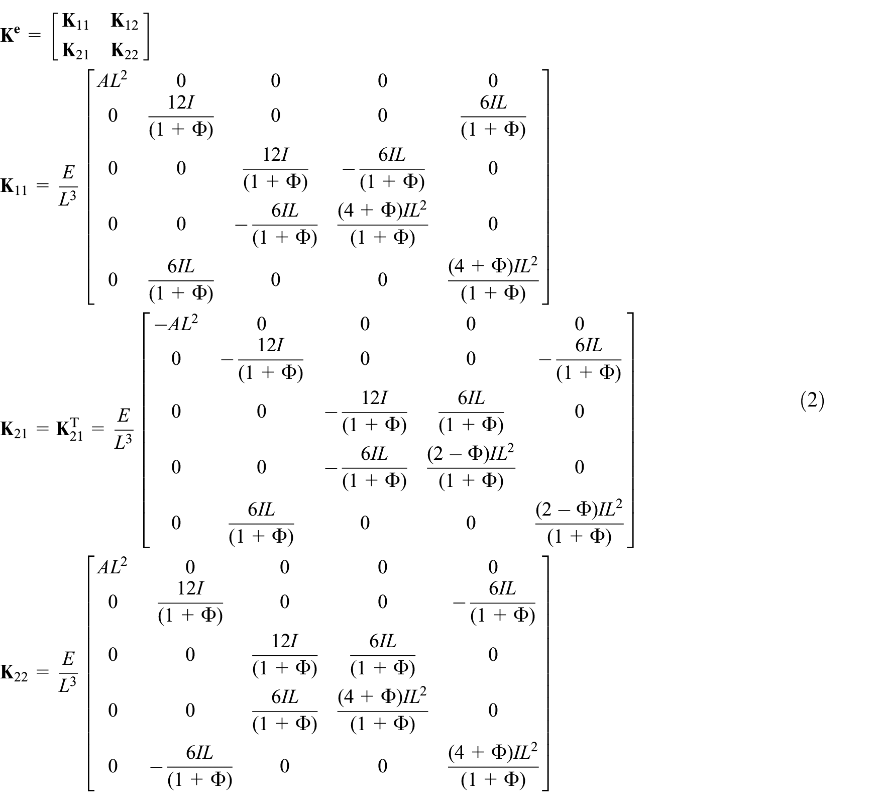
where Φ is the coefficient that concerns the beam shear deflection and is calculated as follows

$$\Phi =\frac{12\mathrm{EI}}{k_s\mathrm{GA}{L}^2}$$

(3)

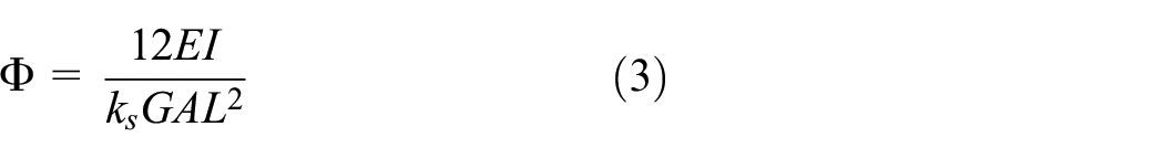
where E is Young’s modulus of the material, k_s is the shear factor set to 0.5 for tube-like beams and G is the shear modulus.

When the inertia and stiffness matrices of each element are obtained and number consecutively, they are assembled to construct the global inertia matrix M and stiffness matrix K of the shaft. Due to the longitudinal axes of all the beams of the shaft are collinear, as shown in Figure 1(b), the matrices of elements can be assembled directly without coordinate transformations

$$\begin{array}{cc}\multicolumn{1}{c}{}& \mathbf{M}=\left[\begin{array}{cccccc}\hfill {\mathbf{M}}_{11}^1\hfill & \hfill {\mathbf{M}}_{12}^1\hfill & \hfill 0\hfill & \hfill 0\hfill & \hfill \cdots \hfill & \hfill 0\hfill \\ \multicolumn{1}{c}{{\mathbf{M}}_{21}^1}& \hfill {\mathbf{M}}_{22}^1+{\mathbf{M}}_{11}^2\hfill & \hfill {\mathbf{M}}_{12}^2\hfill & \hfill 0\hfill & \hfill \cdots \hfill & \hfill 0\hfill \\ \multicolumn{1}{c}{0}& \hfill {\mathbf{M}}_{21}^2\hfill & \hfill {\mathbf{M}}_{22}^2+{\mathbf{M}}_{12}^3\hfill & \hfill \ddots \hfill & \hfill \cdots \hfill & \hfill 0\hfill \\ \multicolumn{1}{c}{⋮}& \hfill ⋮\hfill & \hfill \ddots \hfill & \hfill ⋮\hfill & \hfill {\mathbf{M}}_{22}^{n-1}+{\mathbf{M}}_{11}^n\hfill & \hfill {\mathbf{M}}_{12}^n\hfill \\ \multicolumn{1}{c}{0}& \hfill 0\hfill & \hfill 0\hfill & \hfill \cdots \hfill & \hfill {\mathbf{M}}_{21}^n\hfill & \hfill {\mathbf{M}}_{22}^n\hfill \end{array}\right]\hfill \\ \multicolumn{1}{c}{}& \mathbf{K}=\left[\begin{array}{cccccc}\hfill {\mathbf{K}}_{11}^1\hfill & \hfill {\mathbf{K}}_{12}^1\hfill & \hfill 0\hfill & \hfill 0\hfill & \hfill \cdots \hfill & \hfill 0\hfill \\ \multicolumn{1}{c}{{\mathbf{K}}_{21}^1}& \hfill {\mathbf{K}}_{22}^1+{\mathbf{K}}_{11}^2\hfill & \hfill {\mathbf{K}}_{12}^2\hfill & \hfill 0\hfill & \hfill \cdots \hfill & \hfill 0\hfill \\ \multicolumn{1}{c}{0}& \hfill {\mathbf{K}}_{21}^2\hfill & \hfill {\mathbf{K}}_{22}^2+{\mathbf{K}}_{12}^3\hfill & \hfill \ddots \hfill & \hfill \cdots \hfill & \hfill 0\hfill \\ \multicolumn{1}{c}{⋮}& \hfill ⋮\hfill & \hfill \ddots \hfill & \hfill ⋮\hfill & \hfill {\mathbf{K}}_{22}^{n-1}+{\mathbf{K}}_{11}^n\hfill & \hfill {\mathbf{K}}_{12}^n\hfill \\ \multicolumn{1}{c}{0}& \hfill 0\hfill & \hfill 0\hfill & \hfill \cdots \hfill & \hfill {\mathbf{K}}_{21}^n\hfill & \hfill {\mathbf{K}}_{22}^n\hfill \end{array}\right]\hfill \end{array}$$

(4)

where the superscript of matrices block denotes the first, second, …, nth elements.

Damping coefficients

Damping plays an important role in the dynamic analysis of the structures and foundations. In this article, the damping is treated as an equivalent Rayleigh damping model, which may be expressed as follows

$$\mathbf{C}=\alpha \mathbf{M}+\beta \mathbf{K}$$

(5)

where $\mathbf{C}$ is the damping matrix of the shaft, α and β are pre-defined constants which satisfy the follow equations

$$2{\zeta }_i{\omega }_i=\alpha +\beta {\omega }_i^2$$

(6)

where ζ_i and ω_i are the ith damping ratio in uncoupled mode and ith natural frequency of the system, respectively. As only a first few modes are significantly relevant to the dynamic performance of most engineering structures, α and β could be determined by the following steps: ¹¹ (1) selecting the damping ratios for a first few modes, say ζ₁ to ζ₅ and (2) extracting the corresponding natural frequencies from the system eigenvalue equation, and then linearly interpolating equation (6).

Modelling of the bearings

The stiffness of angular contact ball bearings has a significant influence on the dynamics of a rotating shaft; therefore, the stiffness determination for bearings is critical in the research or design of machine tool spindle systems. A few researchers and bearing vendors have published empirical formulae to determine bearing stiffness. ¹² However, the majority of these models or formulae describe the bearing as a translational stiffness element in radial and axial dimensions. This can only predict in-plane motions transmitted through the bearing. Hernot developed a single 5-DOF bearing model, based on the load–deflection behaviour of the bearing using the Hertzian contact stress theory for point contacts. ¹³ In his research, he also proposed a double 2-DOF angular contact ball bearing for the bearing-shaft system. Hence, a double 5-DOF bearing assembly model could be derived by combining both the models proposed by Hernot.

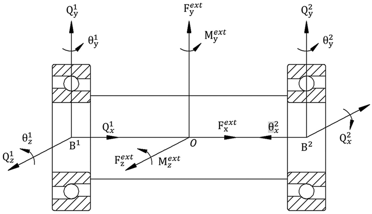
As shown in Figure 3, a 5-DOF bearing has the displacement Q and load F vector, which are as follows

$$\begin{array}{cc}\multicolumn{1}{c}{}& \mathbf{Q}=[Q_x,Q_y,Q_z,{\theta }_y,{\theta }_z{]}^T\hfill \\ \multicolumn{1}{c}{}& \mathbf{F}=[F_x,F_y,F_z,M_y,M_z{]}^T\hfill \end{array}$$

(7)

Figure 3.

Coordinate system and displacements of single 5-DOF bearing.

The load–displacement relationship could be expressed as follows

$$\mathbf{F}=\mathbf{KQ}$$

(8)

The elements of the stiffness matrix K could be calculated as follows

$$\begin{array}{cc}\multicolumn{1}{c}{}& \mathbf{K}=\left[\begin{array}{ccccc}\hfill k_{\mathrm{xx}}\hfill & \hfill k_{\mathrm{xy}}\hfill & \hfill k_{\mathrm{xz}}\hfill & \hfill k_{x{\theta }_y}\hfill & \hfill k_{x{\theta }_z}\hfill \\ \multicolumn{1}{c}{}& \hfill k_{\mathrm{yy}}\hfill & \hfill k_{\mathrm{yz}}\hfill & \hfill k_{y{\theta }_y}\hfill & \hfill k_{y{\theta }_z}\hfill \\ \multicolumn{1}{c}{}& \hfill \hfill & \hfill k_{\mathrm{zz}}\hfill & \hfill k_{z{\theta }_y}\hfill & \hfill k_{z{\theta }_z}\hfill \\ \multicolumn{1}{c}{}& \hfill \mathrm{sym}\hfill & \hfill \hfill & \hfill k_{{\theta }_y{\theta }_y}\hfill & \hfill k_{{\theta }_y{\theta }_z}\hfill \\ \multicolumn{1}{c}{}& \hfill \hfill & \hfill \hfill & \hfill \hfill & \hfill k_{{\theta }_z{\theta }_z}\hfill \end{array}\right]\hfill \\ \multicolumn{1}{c}{}& k_e=\mathrm{Zk}(Q_x\sin \alpha +{\Delta }_r\cos \alpha {)}^{n-1}\hfill \\ \multicolumn{1}{c}{}& k_{\mathrm{xx}}=k_e{\sin }^2\alpha J_a(\epsilon )\hfill \\ \multicolumn{1}{c}{}& k_{\mathrm{xy}}=k_e\sin \alpha \cos \alpha \cos {\phi }_r{J}_{\mathrm{ra}}(\epsilon )\hfill \\ \multicolumn{1}{c}{}& k_{\mathrm{xy}}=k_e\sin \alpha \cos \alpha \sin {\phi }_r{J}_{\mathrm{ra}}(\epsilon )\hfill \\ \multicolumn{1}{c}{}& k_{x{\theta }_y}=k_{\mathrm{xz}}{R}_I\tan \alpha \hfill \\ \multicolumn{1}{c}{}& k_{x{\theta }_z}=-k_{\mathrm{xy}}{R}_I\tan \alpha \hfill \end{array}$$

(9)

$$k_{\mathrm{yy}}=k_e{\cos }^2\alpha ({\sin }^2{\phi }_r{J}_{\mathrm{aa}}(\epsilon )+({\cos }^2{\phi }_r-{\sin }^2{\phi }_r)J_{\mathrm{rr}}(\epsilon ))$$

$$k_{\mathrm{yz}}=k_e{\cos }^2\alpha \sin {\phi }_r\cos {\phi }_r(2J_{\mathrm{rr}}(\epsilon )-J_{\mathrm{aa}}(\epsilon ))$$

$$k_{y{\theta }_y}=k_{\mathrm{yz}}{R}_I\tan \alpha$$

$$k_{y{\theta }_z}=-k_{\mathrm{yy}}{R}_I\tan \alpha$$

$$k_{\mathrm{zz}}=k_e{\cos }^2\alpha ({\cos }^2{\phi }_r{J}_{\mathrm{aa}}(\epsilon )-({\cos }^2{\phi }_r-{\sin }^2{\phi }_r)J_{\mathrm{rr}}(\epsilon ))$$

$$k_{z{\theta }_y}=k_{\mathrm{zz}}{R}_I\tan \alpha$$

$$k_{z{\theta }_z}=-k_{\mathrm{yz}}{R}_I\tan \alpha$$

$$k_{{\theta }_y{\theta }_y}=k_{\mathrm{zz}}{R}_I^2{\tan }^2\alpha$$

$$k_{{\theta }_y{\theta }_z}=-k_{\mathrm{yz}}{R}_I^2\mathrm{ta}{\mathrm{n}}^2\alpha$$

$$k_{{\theta }_z{\theta }_z}=k_{\mathrm{yy}}{R}_I^2{\tan }^2\alpha$$

where Z is the number of balls, α is the contact angle and R_I is the radius of the intersection between the contact cone and the inner raceway median plane. J_aa, J_ra and J_rr are Sjovall’s integrals whose values can be found in a table ¹⁰ for a range of ε. φ_r represents the direction of the maximum radial displacement, and Δ _r is the radial displacement of the inner ring pressure centre, which may be calculated as follows

$$\begin{array}{l}{\phi }_r=\{\begin{array}{c}\mathrm{atan}\left(\frac{Q_z+R_I\tan \alpha {\theta }_y}{Q_y-R_I\tan \alpha {\theta }_z}\right),Q_y-R_I\tan \alpha {\theta }_z>0\\ \mathrm{atan}\left(\frac{Q_z+R_I\tan \alpha {\theta }_y}{Q_y-R_I\tan \alpha {\theta }_z}\right)+\pi ,Q_y-R_I\tan \alpha {\theta }_z\mathrm{<}0\end{array}\\ {\Delta }_r=\sqrt{{(Q_y-R_I\tan \alpha {\theta }_z)}^2+{(Q_z+R_I\tan \alpha {\theta }_y)}^2}\end{array}$$

(10)

As we can observe from the above equations, several elements of the stiffness matrix K are functions of the displacement Q. Hence, given the load and bearing parameters, the displacements cannot be directly calculated. Hence, certain iteration algorithms must be adopted. For example, equation (8) can be modified as follows

$$r=(\mathbf{K}(\mathbf{Q})\mathbf{Q}-\mathbf{F}{)}^2$$

(11)

Next, using an optimization algorithm, a solution Q may be found such that r attains the minimum. Then, the solution Q will be inserted back into equation (9) to determine the stiffness matrix K.

With respect to the bearings assembly shown in Figure 4, three steps are required to obtain the stiffness matrices for the bearings. First, assuming the bearing and shaft system are rigid bodies, the equivalent external force on the centre of the system is determined. Second, according to the geometry consistent condition and the rigid body equilibrium condition, the reaction forces and moments for each bearing are determined. In the final step given the individual reaction forces, equation (11) can be used to find out the displacement of the bearings and their stiffness metrics.

Figure 4.

Coordinate system and displacements of the two 5-DOF bearings arrangement.

The stability lobe diagram

According to Tlusty and colleague,^1,14 whether or not the machining process is stable depends on the cutting depth and its associated spindle speeds. The formula for cutting chip depth b can be expressed as follows

$$b=-\frac{1}{2K_c{N}_t^{*}\mathrm{Re}(G(\omega ))}$$

(12)

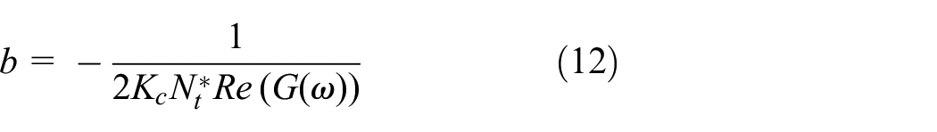
where K_c is the cutting stiffness, $N_t^{*}$ denotes the effective number of teeth in the cut and Re(G(ω)) represents the real part of G(ω), the oriented FRF of the tool nose. The K_c is an empirical coefficient which is dependent on the workpiece material and tool geometry. Both $N_t^{*}$ and G(ω) are related to the cutting geometry and can be determined using the formulas in equation (13) respectively, as depicted in Figure 5 for a down milling application

$$\begin{array}{cc}\multicolumn{1}{c}{}& N_t^{*}=\frac{{\varphi }_{\mathrm{exit}}-{\varphi }_{\mathrm{ent}}}{(2\pi /N_t)}\hfill \\ \multicolumn{1}{c}{}& G(\omega )=-\cos ({\varphi }_{\mathrm{ave}})G_y(\omega )-\sin ({\varphi }_{\mathrm{ave}})G_z(\omega )\hfill \end{array}$$

(13)

Figure 5.

Geometry for determining the effective number of cutting teeth and the oriented FRF.

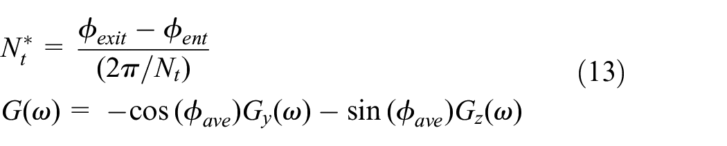
where the angle φ_ent is the entry angle of cutting, φ_exit is the exit angle of cutting, N_t is the real number of the tool, φ_ave is the bisected or average angle of φ_ent and φ_exit, while G_z(ω) and G_y(ω) are the FRFs of the tool nose in Z- and Y-directions. The direction n in Figure 5 is the effective normal direction of the cutting surface in which the cutting chip thickness is calculated to determine the varying cutting force. Obviously, these cutting angles are related to r_d, the radial depth of cut.

From equation (12), it can be determined that the extreme value of b, denoted as b_lim, occurs at the maximum negative value of Re(G(ω)) when frequency $\omega ={\omega }_n\sqrt{1+2\zeta }$ . The b_lim is also referred to as absolute stable cutting depth since keeping the cutting chip depth below b_lim can avoid unstable cutting no matter what spindle speed is chosen. Given the spindle system vibration modes information, the relevant natural frequency ω_n, the damping factor ζ and the stiffness of the mechanical system k can then be determined analytically. Following this, b_lim can be determined using equation (14)

$$b_{\lim }=\frac{2k\zeta (1+\zeta )}{\sin ({\varphi }_{\mathrm{ave}})K_c{N}_t^{*}}$$

(14)

Hence, the key to determining the stable cutting depths is first identifying the FRF of the tool nose. Also, according to regenerative chatter theory, chatter occurs whenever there is a shift of the phase angle ψ between the current and previous surface waviness. ¹⁴ The ratio of the tool vibration frequency ω to the tooth-stroke frequency ω_teeth represents the number of surface waves between consecutive cutter teeth and can be written as follows

$$\begin{array}{cc}\multicolumn{1}{c}{}& \frac{\omega }{{\omega }_{\mathrm{teeth}}}=n+\frac{\psi }{2\pi },n=1,2,\dots \hfill \\ \multicolumn{1}{c}{}& {\omega }_{\mathrm{teeth}}=\Omega N_t\hfill \end{array}$$

(15)

where Ω is the spindle speed. The phase shift angle ψ between the current and previous surface waviness may be expressed as follows

$$\psi =\pi +2\mathrm{atan}\frac{\mathrm{Im}(G(\omega ))}{\mathrm{Re}(G(\omega ))}$$

(16)

where Im(G(ω)) represents the imaginary part of the oriented FRF of the tool nose.

Now that the governing relationships for cutting depth, spindle speeds and chatter have been formulated, the stability lobe diagram can be generated by plotting b_lim within frequency range of interest versus the associated spindle speeds. In the stability diagram, any combination of cutting depth and speed below the lobe curves represents stable cutting parameters while any combination above the lobes indicates unstable cutting.

Stability analysis using Monte Carlo simulation

Monte Carlo simulation uses numerical experimentation to obtain the statistics of a system’s outputs, given the statistics of its input variables. In each experiment, the input random variables are sampled based on their distributions, and the outputs are calculated using the mathematical model of the system. Since each calculation is deterministic when the input random variables have been sampled, the experiments are known as deterministic analysis. However, the data of all experiment results of a large number of deterministic analyses for different sets of values of the input variables will constitute a subset approximating the statistical population of the system’s output.

The procedure of Monte Carlo simulation can be restated as follows. In the first step, values of the system input random variables according to their distribution functions are generated. Then, the deterministic calculation according to the system’s model equation is performed and the results are recorded. The third step involves repeating steps 1 and 2 several times (100–1000 times or even more). The final step involves statistically analysing the previous computation results to find out the interesting features of the system’s statistical performance.

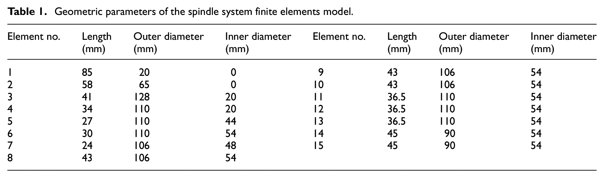
In previous sections, the dynamical modelling procedure of the spindle system has been detailed and according to Figure 1(b), the shaft together with the tool and toolholder have been divided into 15 elements, and the geometric parameters of these elements are listed in Table 1, with the elements numbered from the left to the right. The shaft is made of 38CrMoAlA with a Young’s modulus of E = 2.12 × 10¹¹ Pa.

Table 1.

Geometric parameters of the spindle system finite elements model.

Element no.	Length (mm)	Outer diameter (mm)	Inner diameter (mm)	Element no.	Length (mm)	Outer diameter (mm)	Inner diameter (mm)
1	85	20	0	9	43	106	54
2	58	65	0	10	43	106	54
3	41	128	20	11	36.5	110	54
4	34	110	20	12	36.5	110	54
5	27	110	44	13	36.5	110	54
6	30	110	54	14	45	90	54
7	24	106	48	15	45	90	54
8	43	106	54

By substituting these parameters into equations (1)–(6) and then assembling all the matrices, together with the bearings stiffness matrix, the FRF for the spindle system can be expressed as follows

$$G(\omega )=(-\mathbf{M}{\omega }^2+\mathbf{C}\omega +\mathbf{K}{)}^{-1}$$

(17)

where the damping matrix C was constructed by assuming the damping ratio for the first mode and the sixth mode linearly increasing the mean value from 0.01 to 0.05. These damping ratios were assumed to be random variables with a coefficient of variation of 5%.

In order to complete the stiffness matrix K in equation (17), the stiffness matrix of bearings should be calculated in advance and be added to the stiffness matrix of the shaft at nodes 5 and 10. The tool point was assumed to be subject to the static load F = [900 N, −2000 N, −1800 N, 0, 0] ^T . The axial preload of the bearings was assumed to be a random variable with a coefficient of variation of 5%, and the mean value is 3000 N.

As shown in Figure 6, the Latin hypercube algorithm was used to generate 1000 samples of the bivariate normal distribution for the independent random variables, the damping ratio and the bearing axial preload. Each cross represented a sampled combination of the values of the damping ratio and the bearing axial preload and would be used once in the numerical experimentations to obtain the dynamic performance of the spindle system. The histograms along the abscissa axis and ordinate illustrated the marginal distributions of each variable, respectively. It can be seen that both variables were sampled from a normal distribution. These crosses depicted the joint distribution of the two variables and represented the whole input domain of the Monte Carlo simulations, D. Most of the points in D (about 95%) scattered within the interval of [2700, 3300] for bearing preload and [0.009, 0.011] for damping ratio of the first mode.

Figure 6.

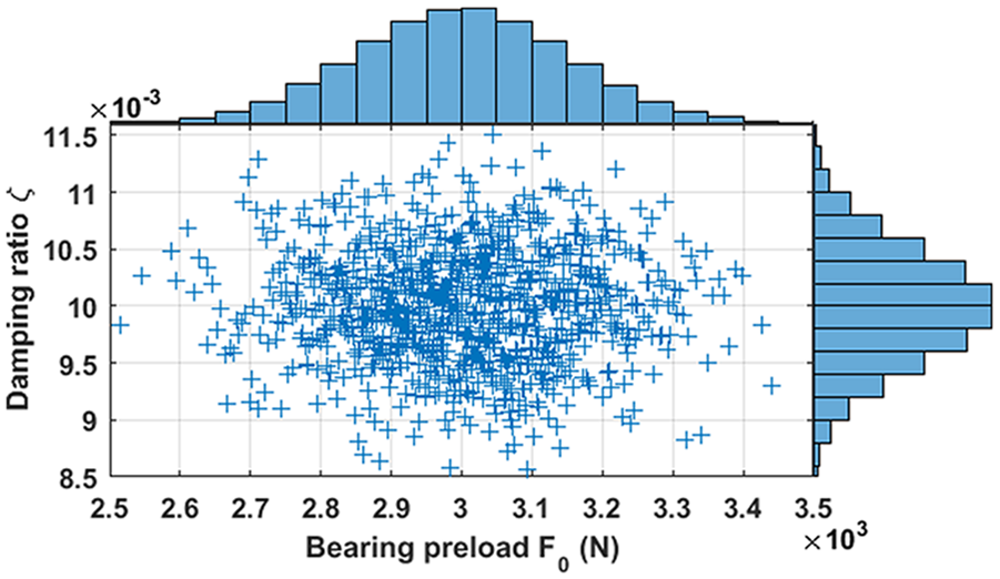
Input domain of the Monte Carlo simulations.

Simulation and experimental results

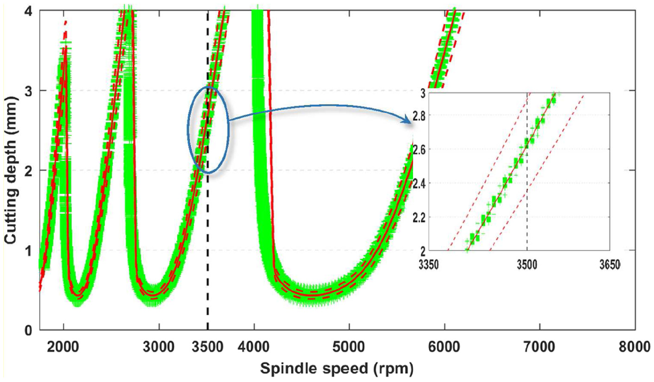
After 1000 deterministic analyses had been carried out, the first modes of the direct FRFs of the tool nose along the Z- and Y-axes were used to generate the stability lobe diagram according to equation (12), as shown in Figure 7. As stated before, the value of the coefficient K_c is related to workpiece material and tool geometry; therefore, it varies from one specific application to another. In this article, the value of K_c is 2410 N/mm², which was obtained by linear regression after a series of cutting tests.

Figure 7.

Stability lobe diagram with the random F0 and random ζ.

The red solid line was plotted with the mean values of the bearing preload and damping ratio, so it represented the nominal stability boundary of the spindle system. In usual applications, machining parameter pairs of the cutting depth and associated spindle speed below the line will be chosen to avoid unstable cutting. A 95% confidence region of the nominal boundary was also plotted with two red dashed lines which were generated according to the so-called two-sigma rule of thumb, which equals the mean values of cutting depth b plus ±2σ. The σ denotes the standard deviation which is the product of the mean value and the coefficient of variation. Then, if the spindle speed is set to 3500 r/min, the nominal stable cutting depth will be 2.58 mm and the maximum stable depth with 95% confidence will be 2.36 mm.

The green crosses which scattered along the nominal stability boundary were obtained using Monte Carlo simulations. Each cross represented a value of output of a Monte Carlo experiment, whose input was a sampled combination of the bearing preload and the damping ratio from the input domain D. Although those crosses shifted a little to the right away from the nominal red line towards higher speeds as the cutting depth increased, they were distributed symmetrically around the nominal stability boundary at fixed speeds. Hence, the proposed spindle model exhibited symmetric response variation when the values of the two chosen parameters varied with normal distribution.

It was evident from Figure 7 that there were a large number of crosses falling outside the 95% confidence region enclosed by the red dashed lines. Therefore, several cutting tests were carried out to verify the stability lobe diagram. A workpiece of carbon steel (ISO C45E4) was machined with a SANDVIK four teeth, 20 mm diameter carbide endmill. The axial cutting depths and associated spindle speeds were represented by blue triangles in Figure 7 and the radial depth of cut was kept constant at 4 mm. The results of cutting tests are shown in Figure 8. Since all the machining parameters were chosen below the red line in Figure 7, stable cutting should be expected. However, as shown in Figure 8, when the spindle speed was 3500 r/min and the cutting axial depths were large than 2.1 mm, the cutting had entered into unstable region.

Figure 8.

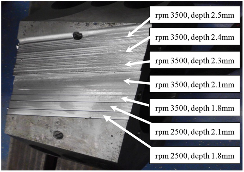
Workpiece of cutting tests.

Through statistical analysis on the data slice at 3500 r/min in Figure 7, it could be find out that there were 69% results of the Monte Carlo simulation lay above 2.36 mm. In other words, when the values of the bearing preload and the damping ratio vary with a coefficient of variation of 5%, it could only guarantee a 69% chance of keeping 2.36 mm below the stable boundaries, as shown in Figure 9.

Figure 9.

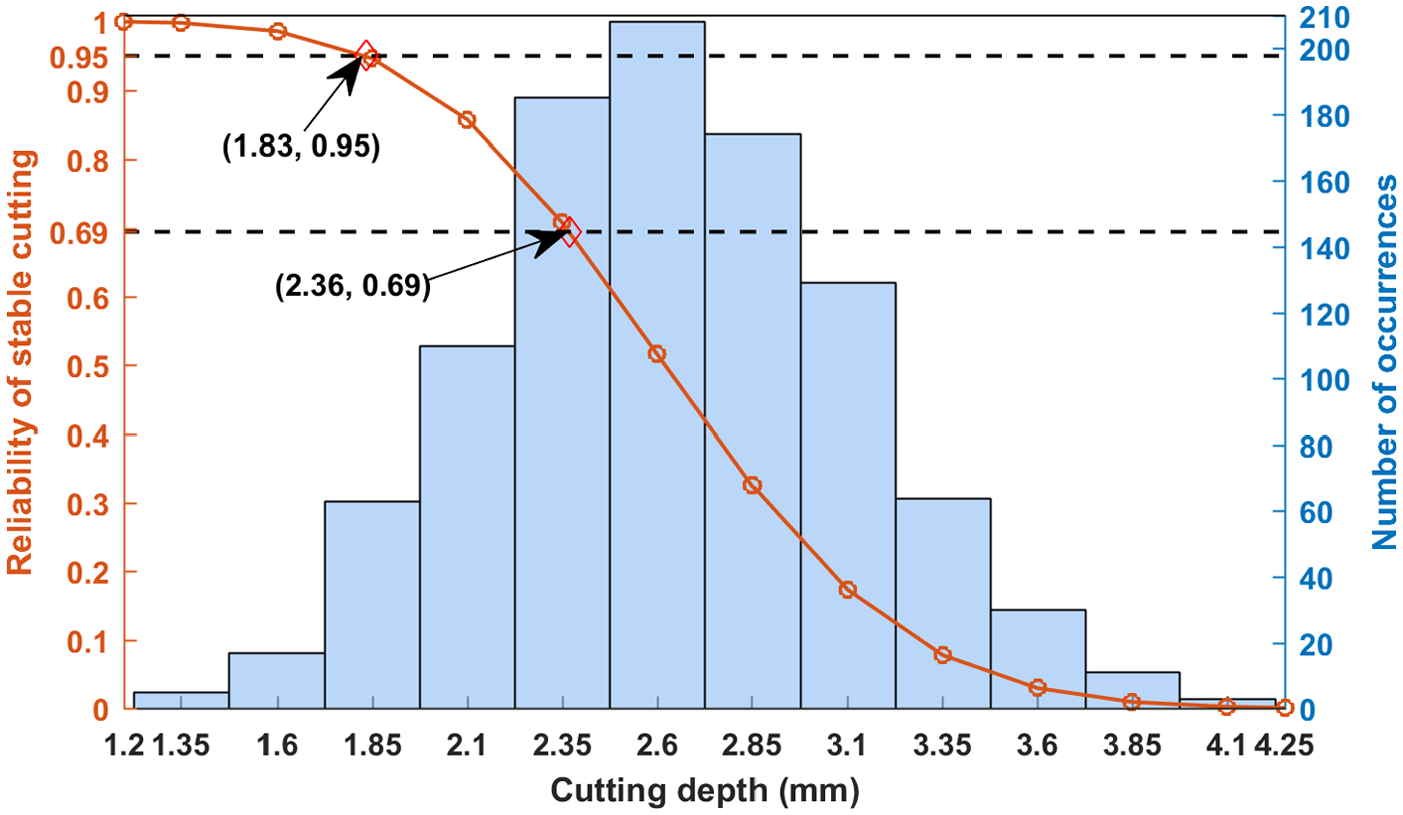
Reliability of stable cutting at spindle speed 3500 r/min.

The histogram in Figure 9 illustrated cutting depth occurrence distribution of 1000 Monte Carl simulations at spindle speed 3500 r/min. The horizontal axis was the cutting depth and the right vertical axis represented the occurrence frequency. The left vertical was the associate reliability of stable cutting. It could be seen that in order to obtain a 95% reliability of avoiding chatter, the cutting depth should be set less than 1.83 mm. This explained why some of the cutting tests got unstable results when the machining parameters were chosen below the nominal stability lobe.

Next, another 1000 Monte Carlo simulations had been carried out, with the bearing preload remaining constant, and only the damping ratio being a random variable. The red solid line was the nominal lobe diagram, which was also lying in the middle of the green crosses. Compared with Figure 7, the simulation results in Figure 10 spread much narrowly. Since the simulations in Figure 7 involved both random variables while the simulations in Figure 10 involved only one, it implied that with the same level of uncertainty (5% coefficient of variation), the damping ratio of the spindle system will not cause large stability prediction errors, while the inaccurate imposed bearing preload should result in the same level of dispersion error in the stability prediction.

Figure 10.

Stability lobe diagram with random ζ.

We can obtain the detail statistical information at any spindle speed as before. For example, by statistical analysing the data slice at 3500 r/min in Figure 10, it could be find out that if the objective was to avoid chatter with a 95% confidence, then the cutting depth should be set below 2.65 mm, as shown in Figure 11.

Figure 11.

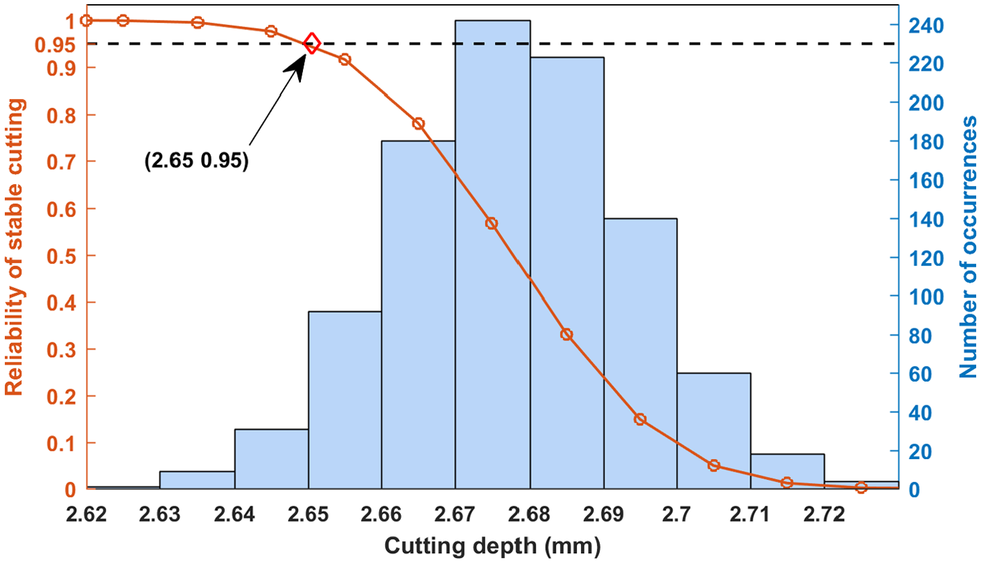
Reliability of stable cutting with random ζ at spindle speed 3500 r/min.

It should be pointed out that the assumption behind the analysis results in Figures 10 and 11 was what we had determined the exact value of the preload of the bearings. However, the cutting tests indicated that the bearing preload had deviated from the nominal value.

Conclusion

The dynamical model of a machine tool spindle system was developed to study its chatter stability, with two key parameters being random variables. The estimation of the true values of these key parameters of the system is challenging, because approximation or uncertainty errors always exist in studies of dynamic engineering systems. If reliability is a crucial specification in the analysis or design application, those uncertainties should be taken into account. The step-by-step modelling process and random sampling simulation method presented in this article provide effective ways to address the uncertainty in engineering analysis. The damping variations do not cause much dispersion or divergence in the spindle stability. However, it is notable that the preloads of bearings, in addition to significantly influencing the static stiffness of a spindle system, also cause fluctuations in its dynamic performance.