Mobile robot nonlinear feedback control based on Elman neural network observer

Abstract

This article presents a new approach to control a wheeled mobile robot without velocity measurement. The controller developed is based on kinematic model as well as dynamics model to take into account parameters of dynamics. These parameters related to dynamic equations are identified using a proposed methodology. Input–output feedback linearization is considered with a slight modification in the mathematical expressions to implement the dynamic controller and analyze the nonlinear internal behavior. The developed controllers require sensors to obtain the states needed for the closed-loop system. However, some states may not be available due to the absence of the sensors because of the cost, the weight limitation, reliability, induction of errors, failure, and so on. Particularly, for the velocity measurements, the required accuracy may not be achieved in practical applications due to the existence of significant errors induced by stochastic or cyclical noise. In this article, Elman neural network is proposed to work as an observer to estimate the velocity needed to complete the full state required for the closed-loop control and account for all the disturbances and model parameter uncertainties. Different simulations are carried out to demonstrate the feasibility of the approach in tracking different reference trajectories in comparison with other paradigms.

Introduction

Many research articles have dealt with the design of control laws for nonholonomic mobile robots. This interest comes from the continuous need for mobile robots in industry, field, and service robots. Mobile robots are no more restricted to factories and some specific places but are becoming closer to human beings when they moved to our homes. More particularly, robots are used to assist people at home or assist disabled individuals if their powered chairs are made intelligent.^1,2 In the early works, the controllers developed for wheeled mobile robots are based on kinematic models. Many works have investigated the trajectory tracking problem using the kinematic model of the mobile robot, and many control laws have been developed including intelligent techniques of the fuzzy logic and neural network. This interest has been extended to dynamic models in order to take into account parameters of dynamics such as mass, moment of inertia, and so on, which might give unforeseen behavior in case they are neglected or badly determined. Based on the dynamic model, many articles focused on tracking and stabilization issues using different types of controllers.^3,4 The controllers developed for this purpose require some accurate knowledge on the parameters to give good performances. In the presence of uncertainties, robust methodologies must be developed in order to meet the imposed performances.^5–7 Moreover, the developed controllers require sensors to obtain the states needed for the closed-loop system. However, some states may not be available due to the absence of the sensors because of the cost, the weight limitation, reliability, induction of errors, failure, and so on. Particularly, for the velocity measurements, the required accuracy may not be achieved in practical applications due to the existence of significant errors induced by stochastic or cyclical noise. For these reasons, software sensors, also called observers, are developed to overcome all the above-cited problems. Tracking control using observers when velocity measurement is not possible has been proposed in some articles.^8–10 In fact, observers constitute the backbone of the system that is to be controlled by estimating the uncertain parameters and compensate for modeling errors and noise. ¹¹ The success and superiority of dynamic neural network over static neural network in system identification and control of dynamical systems^12–17 motivated us to use it as an observer. In this article, Elman neural network (ENN) is proposed for that purpose to estimate the velocity needed to complete the full state required for the closed-loop control. Unlike the static neural network, the ENN has certain dynamical advantages, such as its capability to estimate the velocity in a fraction of the fundamental cycle, avoiding the delay often introduced by static neural networks. When the dynamic model is to be integrated with the nonholonomic kinematics constraints, the problem of trajectory tracking becomes more interesting and more realistic. Motivated by the work of Sarkar et al. ¹⁸ and Yun and Yamamoto, ¹⁹ our goal is to develop a control law approach based on input–output linearization while estimating the nonmeasured system states using ENN trained with the error back-propagation (EBP) algorithm. Thus, the principal contribution of this article is twofold. First, we provide the PowerBot parameter determinations which are necessary in finding the PowerBot dynamic model. Second, the nonmeasured mobile robot velocity is estimated using a proposed ENN observer based on an input–output linearization controller. The proposed observer is inserted to estimate the right and left wheel angular velocities necessary to compute the estimated components of the linear velocity vector. The proposed controller is based on dynamic model. But it seems that PowerBot user interface components do not offer the developer the possibility to access the low-level software but Arcos. Thus, to develop a control software application, one needs to talk to Arcos interface. Further work in this direction is under progress, and only simulation results are presented in this article.

This article is organized as follows. In section “PowerBot parameters determination,” we elaborate the parameter determination of PowerBot, taking into account the physical and mobility parameters that help in determining the inertia tensors and the position of gravity center. The kinematic and dynamic modeling of the mobile robot are presented in section “Kinematic and dynamic modelization.” Section “Mobile robot control” presents the controller’s design for path following. In section “ENN observer,” the proposed procedure of the ENN-based observer is performed for estimating the missing state in the presence of some disturbances. Simulation results are given in section “Simulation results” and section “Conclusion” concludes this article.

PowerBot parameters determination

The PowerBot development platform for this project is one of the most critical components when it comes to successfully achieving the project goals. The project requires us to determine the unknown parameters that serve in elaborating the dynamics model. For this purpose, we propose to give the physical parameters of PowerBot and go through all the steps that lead to the determination of the position of the center of gravity and the different tensors.

PowerBot characteristics

PowerBot, among many research robots developed by Adept Corporation, is a research indoor platform mobile robot. ²⁰ Below, we report the characteristics of PowerBot in terms of its physical and mobility parameters necessary to derive the dynamics model.

Inertia tensors of PowerBot

PowerBot is constituted of elements with different masses and dimensions (Figure 1). Referring to Figure 1, we note that the batteries are fixed in the extreme left robot’s chassis. Therefore, the inertial tensor is not in the geographic center of the robot. For this reason, we propose to split the robot into two rectangular parts as depicted in Figure 2. The first part contains the batteries and the second part the different electronic cards and components.

Figure 1.

Side and top views of PowerBot.

Figure 2.

Center of gravity placements (side view).

The PowerBot characteristics and mobility parameters are defined as follows:

• G _e: center of mass of the electronic cards and components part;

• G_b : center of mass of the batteries part;

• G: center of mass of the robot;

• L: length of the robot: 83.2 cm;

• 2b: width of the Robot: 62.6 cm;

• L_e : length of the electronic part: 43.2 cm;

• L_b : length of the Batteries part: 40 cm;

• L_c : distance from the driving wheel axis to a look ahead reference point P_r: 43 cm;

• H: height of the mobile robot: 48 cm;

• r: drive wheel radius: 27 cm;

• r_c : caster wheel radius: 14 cm;

• m_e : mass of the electronic part: 62 kg;

• m_b : mass of the batteries part: 50 kg;

• m_t : total mass of the electronic and batteries part: 112 kg;

• m_w : mass of each drive wheel: ≅6 kg;

• m_c : mass of each caster wheel: ≅3 kg;

• ${\theta }_l$ : angular position of the front left wheel;

• ${\theta }_r$ : angular position of the front right wheel;

• ϕ: heading angle of the mobile robot;

• I_e : inertia tensor of the electronic part;

• I_b : inertia tensor of the batteries part;

• I_f : inertia tensor of each front driving wheel and the motor rotor;

• I_r : inertia tensor of each rear wheel (caster wheel);

• I_p : inertia tensor of the platform;

• N: transmission ratio = 22.3:1;

• J_r : rotor inertia of one motor = 0.04 kg m².

We calculate the abscissa of the center of mass G as

$$\overline{\mathrm{OG}}=\frac{m_e\frac{L_e}{2}+m_b(L_e+\frac{L_b}{2})}{m_t}$$

(1)

The distance between G and G_b is

$$G{G}_b=\frac{m_b}{2m_t}L$$

The distance between G and G_e is

$$G{G}_e=\frac{m_e}{2m_t}L$$

We obtain the inertia tensors for the electronic part, the batteries part, and the platform as described in the coordinate system of Figure 2, with the origin at the center of mass by applying the parallel axis theorem. Using equation (1), one can determine the abscissa of the center of gravity which is

$$\overline{\mathrm{OG}}=49.1\mathrm{cm}$$

Note that this distance could be slightly different if we take into account the masses of each of the SICK laser sensor, which is equal to 4.5 kg and Bumblebee stereo vision camera, which weights 3 kg. With these values, the center of mass moves backward, and the distance OG would be

$$\overline{\mathrm{OG}}=47.37\mathrm{cm}$$

Now, if the Bumblebee is excluded from calculation, the distance OG becomes

$$\overline{\mathrm{OG}}=48.03\mathrm{cm}$$

The inertia tensors are explained in the following.

Inertia tensor of the platform: I_p

$$I_b=\left[\begin{array}{c}\hfill (4b^2+H^2)\frac{m_b}{12}00\hfill \\ \multicolumn{1}{c}{0(L_b^2+H^2)\frac{m_b}{12}+{\left(\frac{m_{b}L}{2m_t}\right)}^2{m}_{b}0}\\ \multicolumn{1}{c}{00(L_b^2+4b^2)\frac{m_b}{12}+{\left(\frac{m_{b}L}{2m_t}\right)}^2{m}_b}\end{array}\right]$$

(2)

$$I_e=\left[\begin{array}{c}\hfill (4b^2+H^2)\frac{m_e}{12}00\hfill \\ \multicolumn{1}{c}{0(L_e^2+H^2)\frac{m_e}{12}+{\left(\frac{m_{e}L}{2m_t}\right)}^2{m}_{e}0}\\ \multicolumn{1}{c}{00(L_e^2+4b^2)\frac{m_e}{12}+{\left(\frac{m_{e}L}{2m_t}\right)}^2{m}_e}\end{array}\right]$$

(3)

$$I_p=\left[\begin{array}{c}\hfill (4b^2+H^2)\frac{m_t}{12}00\hfill \\ \multicolumn{1}{c}{0\frac{m_t}{12}{H}^2+\frac{m_b{L}_b^2+m_e{L}_e^2}{12}+\frac{L^2}{4m_t^2}(m_b^3+m_e^3)0}\\ \multicolumn{1}{c}{00\frac{m_t}{3}{b}^2+\frac{m_b{L}_b^2+m_e{L}_e^2}{12}+\frac{L^2}{4m_t^2}(m_b^3+m_e^3)}\end{array}\right]$$

(4)

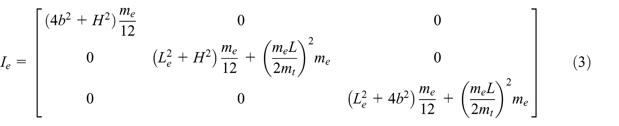
Inertia tensor of each drive wheel: I_f

We consider the wheel as a homogeneous cylinder of radius r and height h. Now, considering the inertia of the motor with respect to its revolution axis, we write the inertia tensor of each front wheel as

$$I_f=\left[\begin{array}{c}\hfill \frac{m_w{r}^2}{4}+\frac{m_w{h}_w^2}{12}00\hfill \\ \multicolumn{1}{c}{0\frac{m_w{r}^2}{2}+N^2{J}_{r}0}\\ \multicolumn{1}{c}{00\frac{m_w{r}^2}{4}+\frac{{\mathrm{mh}}_w^2}{12}}\end{array}\right]$$

(5)

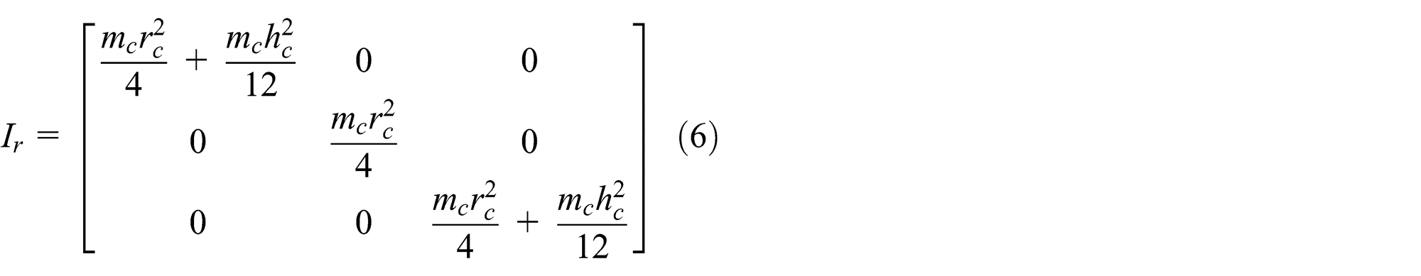
Inertia tensor of each rear (caster) wheel: I_r

We consider the wheel as a homogeneous cylinder of radius r _c and height h_c . The inertia tensor of each caster wheel is written as

$$I_r=\left[\begin{array}{c}\hfill \frac{m_c{r}_c^2}{4}+\frac{m_c{h}_c^2}{12}00\hfill \\ \multicolumn{1}{c}{0\frac{m_c{r}_c^2}{4}0}\\ \multicolumn{1}{c}{00\frac{m_c{r}_c^2}{4}+\frac{m_c{h}_c^2}{12}}\end{array}\right]$$

(6)

Kinematic and dynamic modelization

In the sequel, we use the kinematic model and the dynamic model to determine the motion equation of the robot. All the tensors calculated above will be useful in the equations.

Kinematic model

The model of PowerBot is presented in Figure 3. The model has two diametrically opposed drive wheels of radius r, the distance between the wheels is 2b, the angular speeds of the drive wheels are ω_L and ω_R , and ϕ is the heading angle defined to be the angle between the x-axis attached to the robot and the x-axis of the world coordinates. The coordinates of the center of gravity P_G and the origin of the robot coordinate system P _C are (x_G, y_G ) and (x_C, y_C ), respectively. The distance separating these two points is d. We assume that the mobile robot moves in the direction of the axis of symmetry, and the driving wheels do not sleep while moving. These assumptions can be formulated in a three constraint equations: one is holonomic, and the remaining two are nonholonomic such that

$${\stackrel{·}{y}}_G\cos \varphi -{\stackrel{·}{x}}_G\sin \varphi -d\stackrel{·}{\varphi }=0$$

(7)

$${\stackrel{·}{x}}_G\cos \varphi +{\stackrel{·}{y}}_G\sin \varphi +b\stackrel{·}{\varphi }-r{\stackrel{·}{\theta }}_r=0$$

(8)

$${\stackrel{·}{x}}_G\cos \varphi +{\stackrel{·}{y}}_G\sin \varphi -b\stackrel{·}{\varphi }-r{\stackrel{·}{\theta }}_l=0$$

(9)

Figure 3.

Kinematic model of PowerBot.

To ensure no singularity in the control solution, it has been shown that the point of control P_r cannot be located at the intersection of axis of symmetry of the platform^18,21 but in front of the mobile robot. In the sequel, we will use the three constraints given by equations (7)–(9) and define the configuration of the mobile robot by the vector q of the generalized coordinates which is written as $\mathit{q}={\left[\begin{array}{c}\hfill x_G{y}_G\varphi {\theta }_r{\theta }_l\hfill \end{array}\right]}^T$ .

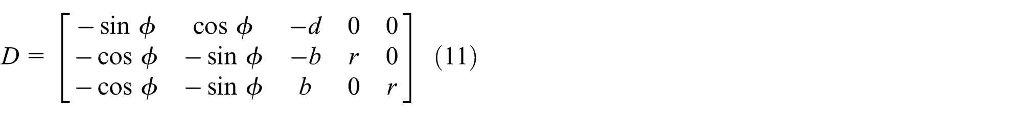
In a more compact form, we write the above three constraint equations in a matrix form as

$$D\left(\mathit{q}\right)\stackrel{·}{\mathit{q}}=0$$

(10)

where

$$D=\left[\begin{array}{c}\hfill -\sin \varphi \cos \varphi -d00\hfill \\ \multicolumn{1}{c}{-\cos \varphi -\sin \varphi -br0}\\ \multicolumn{1}{c}{-\cos \varphi -\sin \varphi b0r}\end{array}\right]$$

(11)

Dynamic model

The dynamic study consists in determining the forces or torques to be applied to the articulations in order to obtain the desired configurations. The standard method that uses the Euler–Lagrange equations is applied in order to obtain the dynamic equations

$$\frac{d}{\mathrm{dt}}\frac{\partial L}{\partial \stackrel{·}{q}}-\frac{\partial L}{\partial q}=E\tau -D^T\lambda$$

(12)

To elaborate the dynamic model, we choose the vector of the generalized coordinates as follows: Our goal is to control the mobile robot over predefined trajectories. Hence, we take x_G and y_G as elements of the vector of the generalized coordinates. However, we want to control the torques of each driving wheel. Therefore, we add the angular position of the driving wheels as elements of this vector. We obtain the following form

$$M\left(q\right)\stackrel{··}{q}+B(q,\stackrel{·}{q})+G\left(q\right)=E\tau -D^T\lambda$$

(13)

where

$$\begin{array}{c}\multicolumn{1}{c}{M\left(q\right)=}\\ \multicolumn{1}{c}{\left[\begin{array}{c}\hfill m_t+2m_{w}02m_{w}d\sin \varphi 00\hfill \\ \multicolumn{1}{c}{0m_t+2m_w-2m_{w}d\cos \varphi 00}\\ \multicolumn{1}{c}{2m_{w}d\sin \varphi -2m_{\mathrm{w}}d\cos \varphi I00}\\ \multicolumn{1}{c}{000I_{f22}0}\\ \multicolumn{1}{c}{0000I_{f22}}\end{array}\right]}\end{array}$$

(14)

The remaining terms are found to be

$$\begin{array}{c}\multicolumn{1}{c}{B(q,\stackrel{·}{q})=\left[\begin{array}{c}\hfill m_{t}d{\stackrel{·}{\varphi }}^2\cos \varphi \hfill \\ \multicolumn{1}{c}{m_{t}d{\stackrel{·}{\varphi }}^2\sin \varphi }\\ \multicolumn{1}{c}{0}\\ \multicolumn{1}{c}{0}\\ \multicolumn{1}{c}{0}\end{array}\right],}\\ \multicolumn{1}{c}{E=\left[\begin{array}{c}\hfill 00\hfill \\ \multicolumn{1}{c}{00}\\ \multicolumn{1}{c}{00}\\ \multicolumn{1}{c}{10}\\ \multicolumn{1}{c}{01}\end{array}\right],\mathrm{and}G\left(q\right)=\left[0\right]}\end{array}$$

$I=I_{p33}+2m_w(b^2+d^2)+2I_{f22}$ and $\tau ={\left[\begin{array}{c}\hfill 000{\tau }_r{\tau }_l\hfill \end{array}\right]}^T$ such that τ_r and τ_l are the torques of the right and left drive wheels, respectively. The vector of Lagrange multipliers is $\lambda =[{\lambda }_{1,}{\lambda }_2{]}^T$ . In order to eliminate the Lagrange multipliers vector λ, we use the angular speeds of the left and right wheels to determine the matrix S(q) such that

$$D\left(q\right)S\left(q\right)=\left[0\right]$$

(15)

Solving the system (15), we obtain the matrix S(q), such that

$$\begin{array}{c}\multicolumn{1}{c}{S\left(q\right)=\left[\begin{array}{c}\hfill s_1\left(q\right)s_2\left(q\right)\hfill \end{array}\right]=}\\ \multicolumn{1}{c}{\left[\begin{array}{c}\hfill c(b\cos \varphi -d\sin \varphi )c(b\cos \varphi +d\sin \varphi )\hfill \\ \multicolumn{1}{c}{c(b\sin \varphi +d\cos \varphi )c(b\sin \varphi -d\cos \varphi )}\\ \multicolumn{1}{c}{c-c}\\ \multicolumn{1}{c}{10}\\ \multicolumn{1}{c}{01}\end{array}\right]}\end{array}$$

(16)

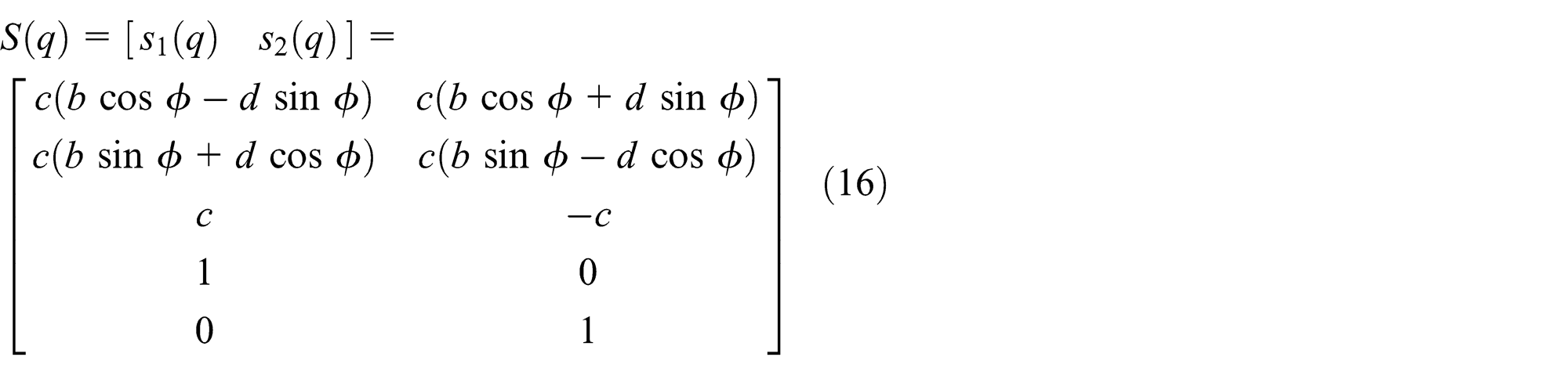
where c = r/2b; hence, the columns of S(q) are in the null space of D, and consequently, S(q) spans N(D). As $\stackrel{·}{q}$ is in the null space of D, there exists a velocity vector ω such that ¹⁸

$$\stackrel{·}{q}=S\left(q\right)\omega$$

(17)

where $\omega =[\begin{array}{c}\hfill {\stackrel{·}{\theta }}_r{\stackrel{·}{\theta }}_l\hfill \end{array}{]}^T$

Multiplying equation (13) by S^T (q), we obtain

$$S^T\left(q\right)E\left(q\right)\left[\begin{array}{c}\hfill {\tau }_l\hfill \\ \multicolumn{1}{c}{{\tau }_r}\end{array}\right]=S^T\left(q\right)M\left(q\right)\stackrel{··}{q}+S^T\left(q\right)B(q,\stackrel{·}{q})$$

(18)

This expression represents the inverse dynamic model of the mobile robot. It helps in elaborating the reference signals to be sent to the motors. We remark that the torques are written in terms of the robot acceleration. However, we are usually interested in controlling the mobile robot in terms of the angular speed and acceleration of the wheels. Thus, we can establish a relation between the motor torques and the system parameters. Deriving equation (17), we obtain

$$\stackrel{··}{q}=\stackrel{·}{S}\left(q\right)\omega +S\left(q\right)\stackrel{·}{\omega }$$

(19)

When substituting $\stackrel{··}{q}$ into equation (18), we obtain

$$\begin{array}{c}\multicolumn{1}{c}{S^{T}E\tau =S^T\left(q\right)M\left(q\right)S\left(q\right)\stackrel{·}{\omega }+S^T\left(q\right)M\left(q\right)\stackrel{·}{S}\left(q\right)\omega }\\ \multicolumn{1}{c}{+S^T\left(q\right)B(q,\stackrel{·}{q})}\end{array}$$

(20)

Mobile robot control

State space representation

Considering the state vector x

$$x={\left[\begin{array}{c}\hfill q\omega \hfill \end{array}\right]}^T$$

(21)

The system state equation (20) can be written as

$$\stackrel{·}{x}=\left[\begin{array}{c}\hfill \stackrel{·}{q}\hfill \\ \multicolumn{1}{c}{\stackrel{·}{\omega }}\end{array}\right]=\left[\begin{array}{c}\hfill S\left(q\right)\omega \hfill \\ \multicolumn{1}{c}{f_2}\end{array}\right]+\left[\begin{array}{c}\hfill \left[0\right]\hfill \\ \multicolumn{1}{c}{{\left(S^T\left(q\right)M\left(q\right)S\left(q\right)\right)}^{-1}{S}^{T}E}\end{array}\right]\tau$$

(22)

Such that $f_2={(S^T\mathrm{MS})}^{-1}{S}^T(-M\stackrel{·}{S}\omega -B)$ .

Once the system is put in its state space form, it can be used for the determination of the control law. By introducing a new input variable u, such that

$$\tau ={\left({(S^T\mathrm{MS})}^{-1}{S}^{T}E\right)}^{-1}(u-f_2)$$

(23)

The state equation given by equation (22) can be further simplified to

$$\stackrel{·}{x}=\left[\begin{array}{c}\hfill \stackrel{·}{q}\hfill \\ \multicolumn{1}{c}{\stackrel{·}{\omega }}\end{array}\right]=\left[\begin{array}{c}\hfill S\left(q\right)\omega \hfill \\ \multicolumn{1}{c}{{\left[0\right]}_{2\times 1}}\end{array}\right]+\left[\begin{array}{c}\hfill {\left[0\right]}_{5\times 1}\hfill \\ \multicolumn{1}{c}{I_{2\times 1}}\end{array}\right]u$$

(24)

In a more compact form, we can write

$$\stackrel{·}{x}=f\left(x\right)+g\left(x\right)u$$

(25)

$$f\left(x\right)=\left[\begin{array}{c}\hfill S\left(q\right)\omega \hfill \\ \multicolumn{1}{c}{f_b}\end{array}\right]$$

(26)

$$g\left(x\right)=\left[\begin{array}{c}\hfill {\left[0\right]}_{5\times 2}\hfill \\ \multicolumn{1}{c}{I_{2\times 2}}\end{array}\right]$$

(27)

System (24) can be partitioned into two subsystems facilitating its analysis and implementation of the control law; we write

$$\{\begin{array}{c}\hfill {\stackrel{·}{x}}_a=f_a\left(x\right)+g_a\left(x\right)u\hfill \\ \multicolumn{1}{c}{{\stackrel{·}{x}}_b=f_b\left(x\right)+g_b\left(x\right)u}\end{array}$$

(28)

Such that

$$\{\begin{array}{c}\hfill f_a\left(x\right)=S\left(q\right)\omega \hfill \\ \multicolumn{1}{c}{f_b\left(x\right)=\left[0\right]}\end{array}$$

(29)

and

$$\{\begin{array}{c}\hfill g_a\left(x\right)=\left[0\right]\hfill \\ \multicolumn{1}{c}{g_b\left(x\right)=I}\end{array}$$

(30)

From system (24), we can identify the time derivative of the state variable x_a and x_b to be

$$\{\begin{array}{c}\hfill {\stackrel{·}{x}}_a=\stackrel{·}{q}\hfill \\ \multicolumn{1}{c}{{\stackrel{·}{x}}_b=\stackrel{·}{\omega }}\end{array}$$

(31)

Then, the system can be expressed into its reduced form

$$\{\begin{array}{c}\hfill {\stackrel{·}{x}}_a=f_a\left(x\right)\hfill \\ \multicolumn{1}{c}{{\stackrel{·}{x}}_b=g_b\left(x\right)u}\end{array}$$

(32)

Nonlinear feedback control

The nonlinear feedback control is used to eliminate nonlinearities present within the system and impose desired linear dynamics. This approach was a success of a large variety of applications. The theory of the nonlinear feedback control has been well established in Slotine and Li ²² and Isidori. ²³ The first application in robotics was introduced on robot manipulators in Tam et al. ²⁴ and extended to mobile robots,^25,26 where the authors showed the usefulness of the approach and revealed its limitations. It is shown in Sarkar et al. ²⁶ that input–output linearization can be achieved using a static state feedback of a reference point whose coordinates are located on the front of the mobile robot and cannot be realized when the point is located at the middle of the axis of symmetry with the driving wheel axis. For this reason, the reference point P_r located in the front side and distant from P_a , by L_r , is chosen as the controlling point. Based on the distance of the center of gravity determined to be equal to 47.37 cm and given the length of the mobile platform L = 83.73 cm, and the distance from the driving wheel axis to a look ahead reference point P_r  = 43 cm, one can deduce the distances d and L_r such that d = 7.17 cm and L_r  = 35.83 cm.

Hence, the output vector is written as

$$y=h\left(x\right)=\left[\begin{array}{c}\hfill x_r\left(q\right)\hfill \\ \multicolumn{1}{c}{y_r\left(q\right)}\end{array}\right]=\left[\begin{array}{c}\hfill x_G+L_r\cos \varphi \hfill \\ \multicolumn{1}{c}{y_G+L_r\sin \varphi }\end{array}\right]$$

(33)

Taking the time derivative of y yields

$$\stackrel{·}{y}=\frac{\partial h}{\partial x}\stackrel{·}{x}=\frac{\partial h}{\partial x}(f\left(x\right)+g\left(x\right)u)$$

(34)

$$\stackrel{·}{y}=L_{f}h\left(x\right)+L_{g}h\left(x\right)u$$

(35)

Letting α = c(d + Lr) and β = c·b, we can verify that

$$L_{f}h\left(x\right)=\left[\begin{array}{c}\hfill -\alpha ({\stackrel{·}{\theta }}_r-{\stackrel{·}{\theta }}_l)\sin \varphi +\beta ({\stackrel{·}{\theta }}_r+{\stackrel{·}{\theta }}_l)\cos \varphi \hfill \\ \multicolumn{1}{c}{\alpha ({\stackrel{·}{\theta }}_r-{\stackrel{·}{\theta }}_l)\cos \varphi +\beta ({\stackrel{·}{\theta }}_r+{\stackrel{·}{\theta }}_l)\sin \varphi }\end{array}\right]$$

(36)

and since L_gh(x) = [0], we compute once more the Lie derivative of equation (35) in order to make the input control u appear in the equation, we obtain

$$\stackrel{··}{y}=L_f^{2}h\left(x\right)+L_g{L}_{f}h\left(x\right)u$$

(37)

$$L_g{L}_{f}h\left(x\right)=\left[\begin{array}{c}\hfill -\alpha \sin \varphi +\beta \cos \varphi \alpha \sin \varphi +\beta \cos \varphi \hfill \\ \multicolumn{1}{c}{\alpha \cos \varphi +\beta \sin \varphi -\alpha \cos \varphi +\beta \sin \varphi }\end{array}\right]$$

(38)

Deriving equation (36), one obtains

$$L_f^{2}h\left(x\right)=\left[\begin{array}{c}\hfill -\alpha c{({\stackrel{·}{\theta }}_r-{\stackrel{·}{\theta }}_l)}^2\cos \varphi -\beta c({\stackrel{·}{\theta }}_r^2-{\stackrel{·}{\theta }}_l^2)\sin \varphi \hfill \\ \multicolumn{1}{c}{-\alpha c{({\stackrel{·}{\theta }}_r-{\stackrel{·}{\theta }}_l)}^2\sin \varphi +\beta c({\stackrel{·}{\theta }}_r^2-{\stackrel{·}{\theta }}_l^2)\cos \varphi }\end{array}\right]$$

(39)

If the matrix L_gLf_h (x) in equation (38) is invertible, then the control vector u can be determined. This is always true since its determinant is always negative: det(L_gLf_h (x)) = −2αβ = −2c ²(d + L_r )b < 0.

Hence, from equation (37), the control law is obtained as

$$u={\left(L_g{L}_{f}h\left(x\right)\right)}^{-1}(\stackrel{··}{y}-L_f^{2}h\left(x\right))$$

(40)

This control law eliminates the nonlinearities and permits to obtain a simple input–output relationship which can stabilize the whole system such that

$$\stackrel{··}{y}=v$$

(41)

Thus, the linearized system is controlled by the outer loop chosen as

$$v=\stackrel{··}{\eta }-K_v\stackrel{·}{e}-K_{p}e$$

(42)

where the vector $\eta ={(x^d,y^d)}^T$ represents the desired trajectories along the x- and y-axes, respectively. The error and its time derivative are the difference between the desired and measured trajectories such that $e=\eta -y$ and $\stackrel{·}{e}=\stackrel{·}{\eta }-\stackrel{·}{y}$ , and K_p and K_v are diagonal gain matrices whose elements are positive and well chosen to assure stability and precision.

Stability analysis

In the preceding section, we have shown that the stability and performance of the linearized system can be realized by a good choice of the gains K_p and K_v . However, the dynamic behavior of the obtained system depends also on the internal dynamics. Since the control law must take into consideration all the dynamics, the internal behavior must be carefully considered. The question is to know whether the internal states stay bounded. The equations which determine internal dynamics are called zero dynamics. They are defined as the dynamics of the system when the state feedback law u ₀ maintains the output y and its time derivatives identically equal to zero, such that

$$u_0=-\frac{L_f^{2}h\left(x\right)}{L_g{L}_{f}h\left(x\right)}$$

(43)

To study the behavior of the internal dynamics, consider the state transformation of the nonlinear system represented by equations (25) and (33). It is transformed to the normal form by constructing the following diffeomorphism, z ₁ = h ₁(x), z ₂ = L_fh ₁(x), z ₃ = h ₂(x), and z ₄ = L_fh ₂(x). Since the variable x is seven dimensional, three more components are added. We choose to complete the vector by adding the right and left wheel angles, z ₅ = θ_l and z ₆ = θ_r , as well as the orientation angle z ₇ = ϕ. However, since z ₇ depends on z ₅ and z ₆, by the relation z ₇ = c(z ₅ − z ₆), the vector z is only six dimensional, z = [h ₁(x), L_fh ₁(x), h ₂(x), L_fh ₂(x), θ_l, θ_r ,] ^T

$$\left[\begin{array}{c}\hfill {\stackrel{·}{z}}_1\hfill \\ \multicolumn{1}{c}{{\stackrel{·}{z}}_2}\\ \multicolumn{1}{c}{{\stackrel{·}{z}}_3}\\ \multicolumn{1}{c}{{\stackrel{·}{z}}_4}\\ \multicolumn{1}{c}{{\stackrel{·}{z}}_5}\\ \multicolumn{1}{c}{{\stackrel{·}{z}}_6}\end{array}\right]=\left[\begin{array}{c}\hfill z_2\hfill \\ \multicolumn{1}{c}{L_f^2{h}_1\left(x\right)}\\ \multicolumn{1}{c}{z_4}\\ \multicolumn{1}{c}{L_f^2{h}_2\left(x\right)}\\ \multicolumn{1}{c}{{\stackrel{·}{\theta }}_r}\\ \multicolumn{1}{c}{{\stackrel{·}{\theta }}_l}\end{array}\right]+\left[\begin{array}{c}\hfill 00\hfill \\ \multicolumn{1}{c}{L_g{L}_{f}h\left(x\right)0}\\ \multicolumn{1}{c}{00}\\ \multicolumn{1}{c}{0L_g{L}_{f}h\left(x\right)}\\ \multicolumn{1}{c}{00}\\ \multicolumn{1}{c}{00}\end{array}\right]\left[\begin{array}{c}\hfill u_1\hfill \\ \multicolumn{1}{c}{u_2}\end{array}\right]$$

(44)

Equations (36) can be rearranged to obtain

$$\left[\begin{array}{c}{L}_f{h}_1\left(x\right)\\ L_f{h}_2\left(x\right)\end{array}\right]=\left[\begin{array}{c}{z}_2\\ z_4\end{array}\right]=\left[\begin{array}{cc}-\alpha \sin \varphi +\beta \cos \varphi & \alpha \sin \varphi +\beta \cos \varphi \\ \alpha \cos \varphi +\beta \sin \varphi & -\alpha \cos \varphi +\beta \sin \varphi \end{array}\right]\left[\begin{array}{c}{\dot{\theta }}_r\\ {\dot{\theta }}_l\end{array}\right]$$

Thus

$$\left[\begin{array}{c}\hfill {\stackrel{·}{\theta }}_r\hfill \\ \multicolumn{1}{c}{{\stackrel{·}{\theta }}_l}\end{array}\right]=\left[\begin{array}{c}\hfill \beta \sin \varphi -\alpha \cos \varphi -\beta \cos \varphi -\alpha \sin \varphi \hfill \\ \multicolumn{1}{c}{-\beta \sin \varphi -\alpha \cos \varphi \beta \cos \varphi -\alpha \sin \varphi }\end{array}\right]\left[\begin{array}{c}\hfill z_2\hfill \\ \multicolumn{1}{c}{z_4}\end{array}\right]$$

(45)

After applying the feedback (40), the system of the mobile robot is written in the following form

$$\begin{array}{c}\multicolumn{1}{c}{\left[\begin{array}{c}\hfill {\stackrel{·}{z}}_1\hfill \\ \multicolumn{1}{c}{{\stackrel{·}{z}}_2}\\ \multicolumn{1}{c}{{\stackrel{·}{z}}_3}\\ \multicolumn{1}{c}{{\stackrel{·}{z}}_4}\\ \multicolumn{1}{c}{{\stackrel{·}{z}}_5}\\ \multicolumn{1}{c}{{\stackrel{·}{z}}_6}\end{array}\right]}\\ \multicolumn{1}{c}{=\left[\begin{array}{c}\hfill 010000\hfill \\ \multicolumn{1}{c}{000000}\\ \multicolumn{1}{c}{000100}\\ \multicolumn{1}{c}{000000}\\ \multicolumn{1}{c}{0\beta \sin \varphi -\alpha \cos \varphi 0-\beta \cos \varphi -\alpha \sin \varphi 10}\\ \multicolumn{1}{c}{0-\beta \sin \varphi -\alpha \cos \varphi 0\beta \cos \varphi -\alpha \sin \varphi 01}\end{array}\right]z}\\ \multicolumn{1}{c}{+\left[\begin{array}{c}\hfill 00\hfill \\ \multicolumn{1}{c}{10}\\ \multicolumn{1}{c}{00}\\ \multicolumn{1}{c}{01}\\ \multicolumn{1}{c}{00}\\ \multicolumn{1}{c}{00}\end{array}\right]v}\end{array}$$

(46)

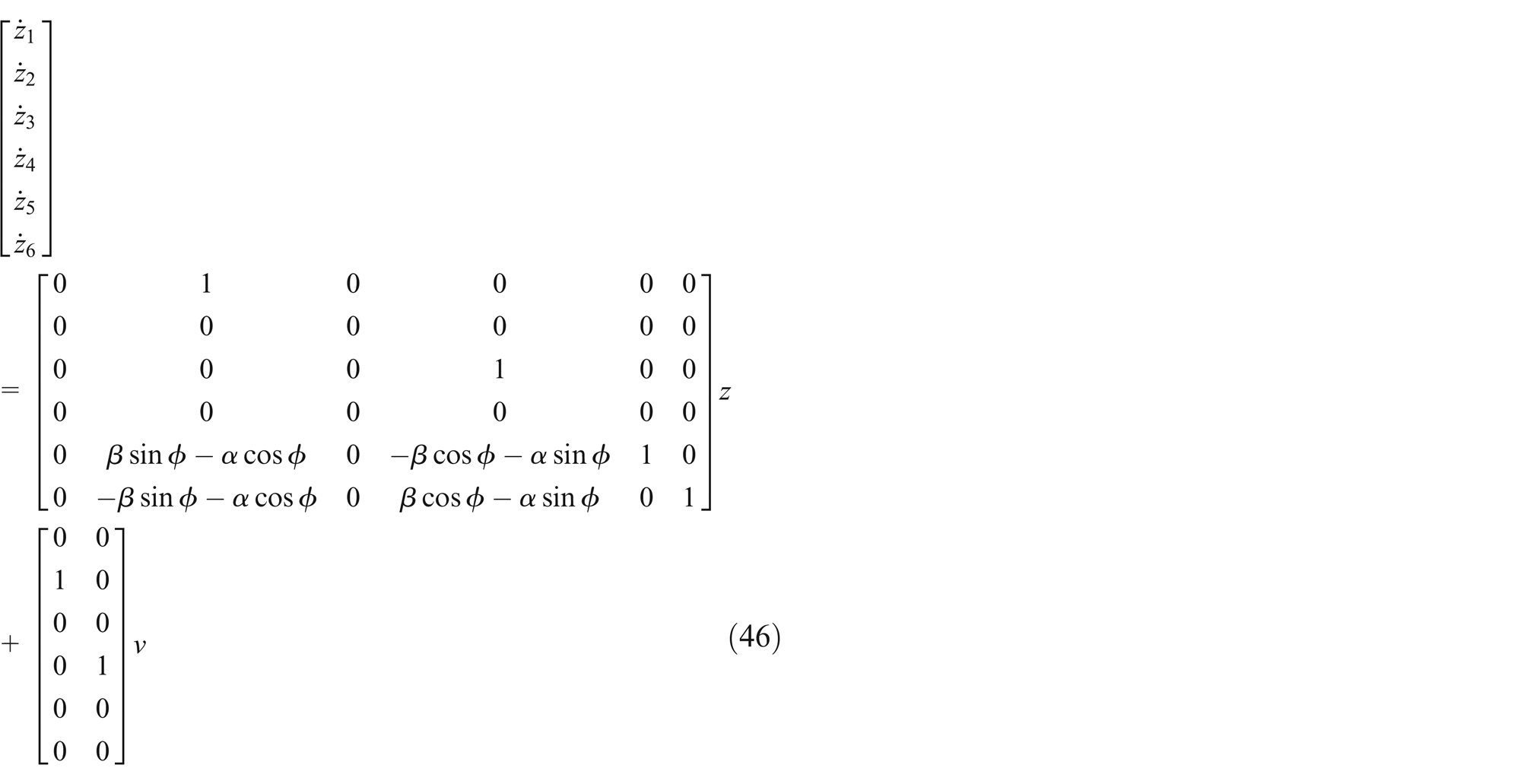
where v can be chosen as in equation (42) or by pole placement, that is, v = −Kz. The internal dynamics associated with the input–output linearization correspond to the two last equations. In this case, the equations are split into two groups, where the second group corresponds to the zero dynamics and written as

$$\left[\begin{array}{c}\hfill {\stackrel{·}{z}}_5\hfill \\ \multicolumn{1}{c}{{\stackrel{·}{z}}_6}\end{array}\right]=\left[\begin{array}{c}\hfill \beta \sin \varphi -\alpha \cos \varphi -\beta \cos \varphi -\alpha \sin \varphi \hfill \\ \multicolumn{1}{c}{-\beta \sin \varphi -\alpha \cos \varphi \beta \cos \varphi -\alpha \sin \varphi }\end{array}\right]\left[\begin{array}{c}\hfill z_2\hfill \\ \multicolumn{1}{c}{z_4}\end{array}\right]$$

(47)

The zero dynamics are defined as the dynamics of the system when the output y and its time derivatives are identically equal to zero, that is, z ₁ = z ₂ = z ₃ = z ₄ = 0. Hence, ${\stackrel{·}{z}}_5={\stackrel{·}{z}}_6=0$ , which means that z ₅ and z ₆ remain constant. Consequently, the zero dynamics are stable but not asymptotically stable. Yun and Yamamoto ²⁷ have shown that the mobile robot has a stable behavior if it moves in the forward direction but an unstable behavior when it has to move backward.

ENN observer

ENN is a partial neural network model that was first proposed for speech processing. ¹² Recently, the ENN has been widely used for the identification and control of dynamical systems. In this section, we propose a design based on this type of recurrent neural network to estimate the time derivative of the mobile robot coordinates. For our convenience, the model expressed by equation (13) can be written in state equation form. Choosing x ₁ = q and $x_2=\stackrel{·}{q}$ as the state variables of the system, the following state representation is obtained

$$\{\begin{array}{c}\hfill {\stackrel{·}{x}}_1=x_2\hfill \\ \multicolumn{1}{c}{{\stackrel{·}{x}}_2=M^{-1}\left(x_1\right)(E\tau -B(x_1,x_2)-D^T\lambda )}\end{array}$$

(48)

If we suppose that only the position state can be measured and the inertial matrix M is approximately known, it imposes the necessity to observe the second state and account for uncertainties. The control law presented in this article is based on only estimating a portion of the second state vector such that ${\hat{x}}_2=({\stackrel{·}{x}}_G,{\stackrel{·}{y}}_G,\stackrel{·}{\varphi },\stackrel{·}{\hat{}}{\theta }_1,\stackrel{·}{\hat{}}{\theta }_2)$ . The assumption used is that there exist a vector W(x) and an optimal parameter vector ${\theta }^{*}$ such that

$$x={\theta }^{*T}W$$

(49)

For our purpose, the Elman recurrent neural network model is chosen as an observer to estimate the nonmeasurable states. It is inserted in the controlled system as shown in Figure 4. The estimated output can be expressed in the following form

$$x^{(2)}={\hat{\theta }}^{T}W$$

(50)

Figure 4.

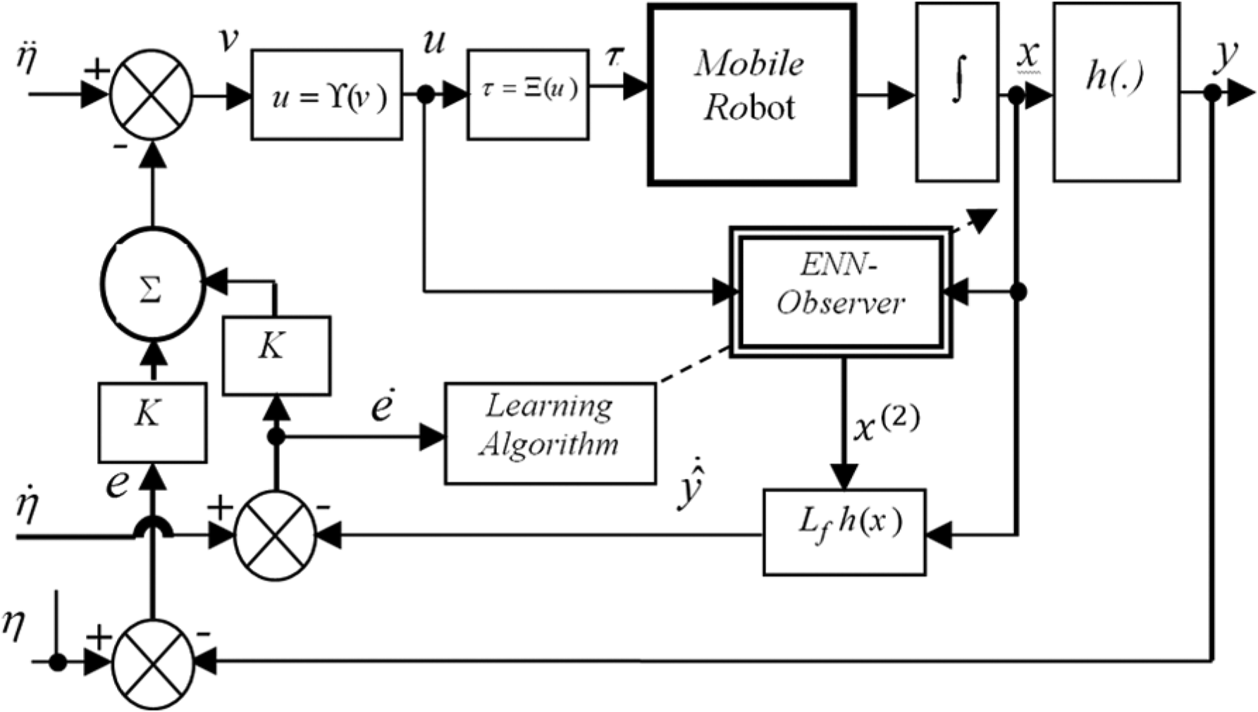
Input–output control with a neural network.

where $\hat{\theta }$ is the parameter vector that is computed when the network is trained using dynamic back-propagation algorithm. The control objective is to force the tracking error between the desired output $\stackrel{·}{\eta }$ and the estimated time derivative output $\stackrel{·}{\hat{}}y$ to converge to a neighborhood of zero. Consider the ENN structure shown in Figure 5. It is a recurrent neural network with four layers of neurons, namely, input layer, hidden layer, context layer, and output layer. The structure has an output layer weight matrix $W^{(0)}$ whose elements connect the hidden layer to the output layer, and a hidden layer weight matrix $W^{(0)}=[W^{(0i)},W^{(0c)}]$ consisted of two sub-weight matrices $W^{(0i)}\mathrm{and}{W}^{(0c)}$ , whose elements connect the input layer and the context layer to the hidden layer, respectively.

Figure 5.

Structure of the ENN.

Input layer

In this layer, the input variables are the measured position and orientation of the mobile robot: $(x_G,y_G,\varphi )$ , and the corresponding computed controller vector: $(u_r,u_l)$ .

Context layer

The context layer behaves like the input layer. The context node input values are simply the calculated values of the hidden output nodes transmitted via recurrent connections through a unit delay, that is, ${\mathit{x}}^{(1)}(t-1)$ . Thus, the number of context nodes is equal to the hidden layer neurons. In this case, the input data of the input layer 0 are ${\mathit{x}}^{(0)}=(x_G,y_G,\varphi ,u_{\mathrm{r}},u_l,{\mathit{x}}^{(1)}(t-1),\rho x_c^{(0)}(t-1))$ , such that ${\mathit{x}}^{(1)}(t-1)$ and $\rho x_c^{(0)}(t-1)$ denote the output signals of the hidden and context neurons in the previous time, respectively, and $0\le \rho <1$ is the self-connecting feedback gain.

Hidden layer

In this layer, each neuron is described by an activation sigmoid function. The number of hidden layer neurons is equal to m. This number is chosen arbitrary; one can always begin with a minimum number of nodes and keep increasing until no more improvement could be seen. The output ${\mathit{x}}_i^{(1)}$ of the ith hidden neuron can be expressed as

$${\mathit{x}}_i^{(1)}=\frac{2}{1+e^{-4(\mathrm{ne}{t}_i)}}-1$$

(51)

where

$$\mathrm{ne}{t}_i={\displaystyle \sum _{j=1}^{m+5}}{W}_{\mathrm{ij}}^{(0)}{x}_j^{(0)}i=1,\dots ,m=7$$

(52)

$W^{(0)}$ is the matrix that includes the connections weights between the input–context layers and the hidden layer.

Output layer

In this application, only terms that cannot be measured are estimated. Therefore, only a portion of the second state vector is observed, that is, ${\mathit{x}}^{(2)}=[{\widehat{\stackrel{·}{\theta }}}_1,{\widehat{\stackrel{·}{\theta }}}_2{]}^T$ . Each neuron of the output layer is described by an activation linear function, and the output of the jth output is expressed as

$${\mathit{x}}_i^{(2)}={\hat{x}}_{2i}=G\times \left(\mathrm{ne}{t}_i\right),i=1,2$$

(53)

where G is a certain chosen gain and $\mathrm{ne}{t}_i={\displaystyle \sum _{j=1}^{m=7}}{W}_{\mathrm{ij}}^{(1)}{x}_j^{(1)}$ , such that $W^{(1)}$ is the matrix that includes the connection weights between the hidden and output layers. We can define the measured error as the squared error between the desired output and the estimated output defined as

$$E=\frac{1}{2}{\Vert \dot{\eta }-\dot{\widehat{y}}\Vert }^2=\frac{1}{2}\left({\left({\dot{x}}^d-{\dot{\widehat{y}}}_1\right)}^2+{\left({\dot{y}}^d-{\dot{\widehat{y}}}_2\right)}^2\right)$$

(54)

The aim is to find the appropriate weights by minimizing the error E. The output error signals are found by taking the ordered derivative given by the expression

$$\begin{array}{l}{\epsilon }_{2,i}=\frac{{\partial }^{+}E}{\partial x_i^{(2)}}=\frac{\partial E}{\partial x_i^{(2)}}=\frac{\partial E}{\partial {\dot{\widehat{y}}}_1}\frac{\partial {\dot{\widehat{y}}}_1}{\partial x_i^{(2)}}+\frac{\partial E}{\partial {\dot{\widehat{y}}}_2}\frac{\partial {\dot{\widehat{y}}}_2}{\partial x_i^{(2)}}\\ {\epsilon }_{2,i}=-\left({\dot{x}}^d-{\dot{\widehat{y}}}_1\right)\frac{\partial {\dot{\widehat{y}}}_1}{\partial x_i^{(2)}}-\left({\dot{y}}^d-{\dot{\widehat{y}}}_2\right)\frac{\partial {\dot{\widehat{y}}}_2}{\partial x_i^{(2)}}\end{array}$$

(55)

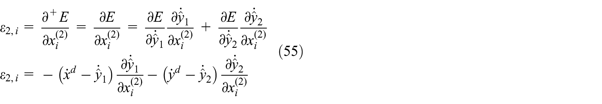
Proceeding with each error signal, we obtain

$$\begin{array}{l}{\epsilon }_{2,1}=-\left({\dot{x}}^d-{\dot{\widehat{y}}}_1\right)\left(-\alpha \sin \varphi +\beta \cos \varphi \right)-\left({\dot{y}}^d-{\dot{\widehat{y}}}_2\right)\left(\alpha \cos \varphi +\beta \sin \varphi \right)\\ {\epsilon }_{2,2}=-\left({\dot{x}}^d-{\dot{\widehat{y}}}_1\right)\left(\alpha \sin \varphi +\beta \cos \varphi \right)-\left({\dot{y}}^d-{\dot{\widehat{y}}}_2\right)\left(-\alpha \cos \varphi +\beta \sin \varphi \right)\end{array}$$

(56)

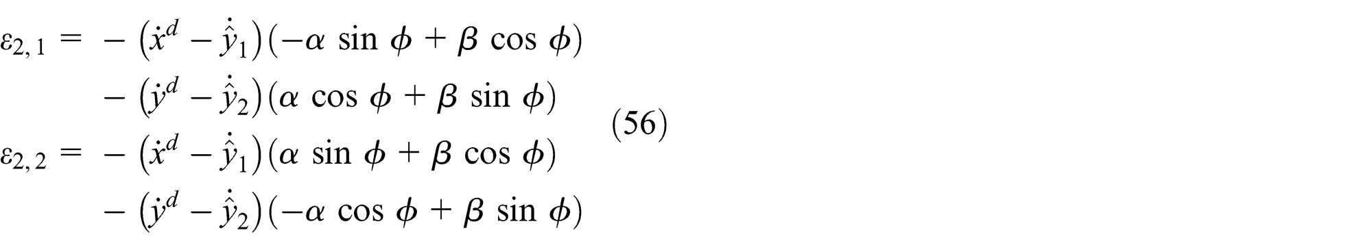
For the hidden, input, and the context layer nodes, the error signals can be derived using the functional decomposition rule

$${\epsilon }_{l,i}={\displaystyle \sum _{j=1}^{N(l+1)}}{\epsilon }_{l+1,j}\frac{\partial x_j^{(l+1)}}{\partial x_i^{(l)}}$$

(57)

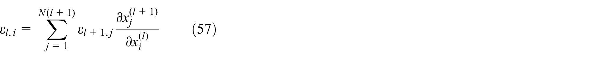
where N(l + 1) is the number of neurons in layer (l + 1). One can verify that the obtained error signal back to the hidden layer is obtained as

$${\epsilon }_{1,i}={\displaystyle \sum _{j=1}^{n=5}}{\epsilon }_{2,j}\frac{\partial x_j^{(2)}}{\partial x_i^{(1)}},i=1,\dots ,7$$

(58)

Proceeding with the calculations, one can find

$${\epsilon }_{1,i}={\displaystyle \sum _{j=1}^{n=5}}{\epsilon }_{2,j}{W}_{\mathrm{ji}}^{(1)},i=1,\dots ,7$$

(59)

The error signal back propagated to the input layer is obtained as

$$\begin{array}{c}\multicolumn{1}{c}{{\epsilon }_{0,i}={\displaystyle \sum _{j=1}^{m=7}}{\epsilon }_{1,j}\frac{\partial x_j^{(1)}}{\partial x_i^{(0)}}={\displaystyle \sum _{j=1}^{m=7}}{\epsilon }_{1,j}\frac{\partial x_j^{(1)}}{\partial \left(\mathrm{ne}{t}_j\right)}\frac{\partial \left(\mathrm{ne}{t}_j\right)}{\partial x_i^{(0)}}}\\ \multicolumn{1}{c}{i=1,\dots ,12}\end{array}$$

(60)

It can be easily shown that

$$\begin{array}{c}\multicolumn{1}{c}{{\epsilon }_{0,i}={\displaystyle \sum _{j=1}^{m=7}}{\epsilon }_{1,j}\frac{\partial x_j^{(1)}}{\partial x_i^{(0)}}=\frac{1}{2}{\displaystyle \sum _{j=1}^{m=7}}{\epsilon }_{1,j}(1-{\left(x_j^{(1)}\right)}^2)W_{\mathrm{ji}}^{(0)}}\\ \multicolumn{1}{c}{i=1,\dots ,12}\end{array}$$

(61)

The Elman back-propagation algorithm is used to update the output and hidden layers recursively at each iteration so that E (t) is minimized. Momentum method is used to accelerate the convergence of the EBP learning algorithm. In this case, a fraction of the most recent weight adjustment is added according to the following formula

$$W_{ij}^{(l)}\left(t+1\right)=W_{ij}^{(l)}\left(t\right)-\alpha \frac{{\partial }^{+}E}{\partial W_{ij}^{(l)}\left(t\right)}+\beta \Delta W^{(l)}\left(t\right),forl=0,1$$

(62)

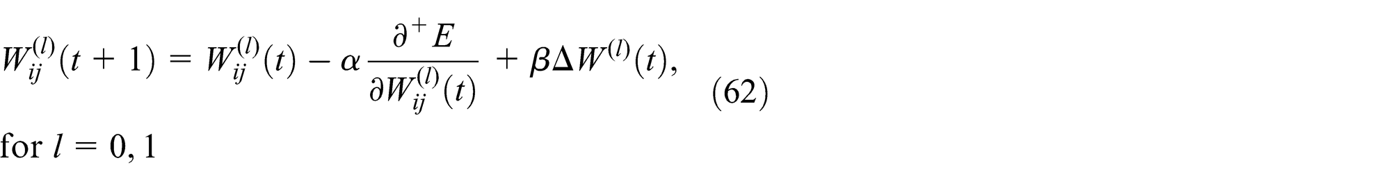
where α is the learning rate coefficient of the EBP and β is a user-selected positive momentum constant typically chosen between 0.1 and 0.9. The third term can be determined as follows

$$\frac{{\partial }^{+}E}{\partial W_{\mathrm{ij}}^{(l)}}=\frac{{\partial }^{+}E}{\partial x_i^{(l+1)}}\times \frac{\partial x_i^{(l+1)}}{\partial W_{\mathrm{ij}}^{(l)}}={\epsilon }_{(l+1),i}\times \frac{\partial x_i^{(l+1)}}{\partial W_{\mathrm{ij}}^{(l)}}$$

(63)

For the hidden-to-output layer weight adjustment: l = 1

$$\frac{{\partial }^{+}E}{\partial W_{\mathrm{ij}}^{(1)}}={\epsilon }_{2,i}\times \frac{\partial x_i^{(2)}}{\partial W_{\mathrm{ij}}^{(1)}}={\epsilon }_{2,i}{x}_j^{(1)}$$

(64)

For the input-to-hidden layer weight adjustment: l = 0

$$\begin{array}{c}\multicolumn{1}{c}{\frac{{\partial }^{+}E}{\partial W_{\mathrm{ij}}^{(0)}}={\epsilon }_{1,i}\times \frac{\partial x_i^{(1)}}{\partial W_{\mathrm{ij}}^{(0)}}={\epsilon }_{1,i}\frac{\partial x_i^{(1)}}{\partial \mathrm{ne}{t}_i}\times \frac{\partial \mathrm{ne}{t}_i}{\partial W_{\mathrm{ij}}^{(0)}}}\\ \multicolumn{1}{c}{=\frac{1}{2}{\epsilon }_{1,i}(1-{\left(x_i^{(1)}\right)}^2)x_j^{(0)}}\end{array}$$

(65)

Simulation results

We present in this section the computer simulation results. The mobile robot is supposed to track two different reference trajectories, namely, a straight line path and a circular path (cf. Figures 6 and 7, respectively). These trajectories are purposely chosen to be analogous to those found in Coelho and Nunes. ⁷ In the presented simulations, the system is linked with the observer based on an ENN design. The training algorithm is carried out through a back-propagation algorithm. The gradient of the objective function with respect to neural network parameters is calculated and used to update the weight parameters, starting from the output layer and propagating backward. To accelerate convergence, a momentum term is being added to the learning expression. The values of the learning rates depend on the problem being solved since the convergence depends significantly on these values. Hence, there is a tradeoff between small values and large values. Small values may lead to the solution but with a small convergence rate; however, large values may overshoot the solution. After some trials, the values retained in this application are found to be α = 0.8 and β = 0.3. We consider errors of 10% on all parameters of the system in order to test the robustness of the proposed scheme with respect to the parametric and structural errors. Simulation results are performed for a specific initial condition which incorporates the true nonlinear nature of the problem with the gains K_p  = 3 and K_v  = 7. In all the experiments, the velocities are reconstructed from the observer. In Figure 6, the initial pose of the mobile robot is (0°, 0°, 90°), while in Figure 7, the initial pose is (5°, 30.6°, 225°). In both cases, the mobile robot tries in the first step to cancel the position error by rapidly approaching the reference paths. Once the paths are reached, the path following is achieved in a well-stable behavior. This tracking behavior is observed in Figures 8 and 9, which show the distance error between the actual and the desired paths. Figures 10 and 11 depict the evolution of the heading angles in both cases. In fact, in case of a straight line path tracking, the transient angle lasts about 8 s before the heading angle stabilizes to a fixed positive value of 45°. However, this angle is observed to increase linearly as the mobile robot turns around the circular path. Note that the desired paths are followed with the mobile robot in the forward motion and the measured forward measured linear velocities are depicted in Figures 12 and 13. The estimated and measured angular velocities of the right wheels are shown in Figures 14 and 15 for the straight line and circular paths, respectively. Figures 16 and 17 depict those of the left wheels for both tracking paths. The curves of the estimated angular speeds attained the measured ones after small lapse of time, which prove the convergence of the ENN observer. The simulation carried on the established model of the mobile robot showed the feasibility of the approach and the successfulness of the observer in estimating the missing states of a system subjected to error modeling.

Figure 6.

Evolution of the mobile robot along a straight line trajectory.

Figure 7.

Evolution of the mobile robot along a circular trajectory.

Figure 8.

Distance error between actual and desired paths performed by the mobile robot in following a straight line path.

Figure 9.

Distance error between actual and desired paths performed by the mobile robot in following a circular path.

Figure 10.

Heading angle plot.

Figure 11.

Heading angle plot.

Figure 12.

Forward velocity of the mobile robot in following a straight line path.

Figure 13.

Forward velocity of the mobile robot in following a circular path.

Figure 14.

Estimated and measured right wheel speeds of the mobile robot in following a straight line path.

Figure 15.

Estimated and measured left wheel speeds of the mobile robot when tracking a circular path.

Figure 16.

Estimated and measured right wheel speeds of the mobile robot in following a straight line path.

Figure 17.

Estimated and measured left wheel speeds of the mobile robot in following a circular path.

Conclusion

The theoretical work in the field of wheeled mobile robot control is large and offers different solutions to solve the problems of displacement. However, the integration of the control laws on an experimental requires us to take into account certain constraints. We presented in this article the different steps in the design, modeling, and control of a mobile robot modular wheel. We initially identify important parameters for the control of mobile robot. This allowed us to make choices not only on the assumptions of behavior but also on the formalism adopted for the kinematic and dynamic modeling. In this article, feedback linearizing control law is used to allow tracking a specified reference trajectory. It is supposed that only the position state can be measured, and some of the parameters that intervene in the modelization are approximately known. To solve these problems, an ENN-based observer is proposed to estimate the nonmeasured velocity vector of the mobile robot. Simulations are carried out and the results obtained show that the complete controlled system presented good performances and stability under uncertainties on the model parameters, which confirm the feasibility of the approach. Further work in this direction is under progress, and our goal is to build the controller on the true PowerBot and carry out the experimental tests.