Model-free active input–output feedback linearization of a single-link flexible joint manipulator: An improved active disturbance rejection control approach

Abstract

Traditional input–output feedback linearization requires full knowledge of system dynamics and assumes no disturbance at the input channel and no system’s uncertainties. In this paper, a model-free active input–output feedback linearization technique based on an improved active disturbance rejection control paradigm is proposed to design feedback linearization control law for a generalized nonlinear system with a known relative degree. The linearization control law is composed of a scaled generalized disturbance estimated by an improved nonlinear extended state observer with saturation-like behavior and the nominal control signal produced by an improved nonlinear state error feedback. The proposed active input–output feedback linearization cancels in real-time fashion the generalized disturbances which represent all the unwanted dynamics, exogenous disturbances, and system uncertainties and transforms the system into a chain of integrators up to the relative degree of the system, which is the only information required about the nonlinear system. Stability analysis has been conducted based on the Lyapunov functions and revealed the convergence of the improved nonlinear extended state observer and the asymptotic stability of the closed-loop system. Verification of the outcomes has been achieved by applying the proposed active input–output feedback linearization technique on the single-link flexible joint manipulator. The simulations results validated the effectiveness of the proposed active input–output feedback linearization tool based on improved active disturbance rejection control as compared to the conventional active disturbance rejection control–based active input–output feedback linearization and the traditional input–output feedback linearization techniques.

Introduction

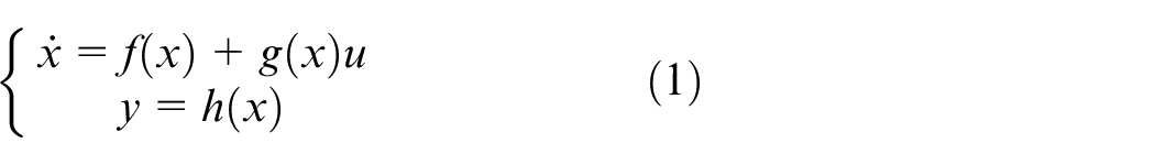
There are numerous classes of nonlinear models, given the following one

$$\{\begin{array}{c}\stackrel{·}{x}=f\left(x\right)+g\left(x\right)u\hfill \\ \multicolumn{1}{c}{y=h\left(x\right)}\end{array}$$

(1)

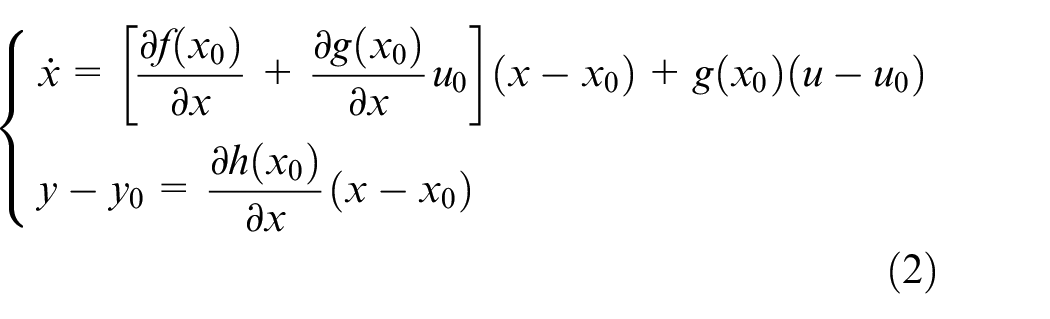
where $x=(x_1{x}_2\dots x_2{)}^T\in {\mathbb{R}}^n$ is the state vector, $u\in \mathbb{R}$ is the control input, and $y\in \mathbb{R}$ is the system output. The functions $f,g,\mathrm{and}h$ are sufficiently smooth in a domain $D\subset {\mathbb{R}}^n$ . The mappings $f:D\to {\mathbb{R}}^n$ and $g:D\to {\mathbb{R}}^n$ are called vector fields on D. Consider the Jacobian linearization of system (1) about the equilibrium point $(x_0.y_0.u_0)$

$$\{\begin{array}{c}\stackrel{·}{x}=[\frac{\partial f\left(x_0\right)}{\partial x}+\frac{\partial g\left(x_0\right)}{\partial x}{u}_0](x-x_0)+g\left(x_0\right)(u-u_0)\hfill \\ y-y_0=\frac{\partial h\left(x_0\right)}{\partial x}(x-x_0)\hfill \end{array}$$

(2)

It is worthy to observe that the nonlinear system is accurately represented by the Jacobian model only at the equilibrium point $(x_0,y_0,u_0)$ . Consequently, any control policy built on the linearized model may produce unacceptable performance at other operating points. Input–output feedback linearization (IOFL) is another class of nonlinear control methods that can yield linear models, that is, a precise depiction of the fundamental nonlinear model among a wide set of the equilibrium points. ¹ IOFL is a technique which eliminates all the nonlinearities with the result that the nonlinear dynamical system is represented by a chain of integrators. IOFL can be applied in the following three steps. The first step is transforming the nonlinear system into a linearized model; this is achieved through an appropriate nonlinear change of variables. After this stage, the equations of the system are linear but with the cost of a linearization control law (LCL) (u) which converts the system into a chain of integrators up to the relative degree of the system with linear control law (v). The second step is applying one of the traditional linear control methods such as state feedback, proportional–integral–derivative (PID) control, and so on, to design a linear control law (v) to control the linearized model. The third step is the stability investigation of the internal dynamics. ²

IOFL has been applied in recent years in various research and industrial fields, for example, in the control of induction motors, ³ spacecraft models that include reaction wheel configuration, ⁴ and surface permanent magnet synchronous generator (SPMSG). ⁵ Further applications include maximum power point tracking (MPPT) technique to achieve the desired performance under sudden irradiation drops, setpoint changes, and load disturbances, ⁶ adaptive input–output feedback linearization to damp the low-frequency oscillations in power systems, ⁷ and for the reduction of torque ripple of brushless direct current (DC) motors, ⁸ and finally, in robust nonlinear controller design for the voltage-source converters of high voltage, DC transmission link using IOFL and sliding mode control approach. ⁹

Active methods for feedback linearization of nonlinear systems have been addressed by many researchers using adaptive control techniques such as approximating the nonlinear function $f(x)$ using the Gaussian radial basis function neural networks (RBF-NNs) ¹⁰ or a particular form of a Brunovsky type neuro-fuzzy dynamical system (NFDS). ¹¹ Simple output feedback adaptive control scheme is developed in Zhou et al. ¹² for a general class of nonlinear systems preceded by an actuator with hysteresis nonlinearity, where a new hysteresis inverse is obtained for the hysteresis and is used to efficiently cancel the hysteresis effects when developing the control scheme with the backstepping approach. An adaptive output feedback control methodology for nonaffine minimum-phase nonlinear systems using nonlinearly parameterized single hidden layer neural networks (SH-NNs) as approximation model is presented in Hovakimyan et al., ¹³ with the assumption that the system is globally exponentially minimum phase. Other recent scenarios for output tracking control can be found in previous studies^14–18 and the references therein. Several nonlinear models can be considered for the proposed control technique in this paper such as aircraft engine, ¹⁹ maglev train,^20–22 unmanned aerial vehicle (UAV), ²³ and pneumatic artificial muscles (PAMs). ²⁴

Although the aforementioned approaches of adaptive control methods^10–13 have much higher power and significantly enhance the ability of a feedback system in dealing with uncertainty beyond robust control, nevertheless, this enhancement is obliged by the variation rates of the system parameters, and performance worsens quickly when the variation rates reach a specific limit. ²⁵ This traditional method to deal with deterministic adaptive control has some intrinsic restrictions which have been very much perceived in the literature^14,26 and the references therein. Most remarkably, if unknown parameters vary in intricate manners, it might be extremely hard to develop a “continuously parameterized” group of competitor controllers. Moreover, adaptation continuously over a period of time may likewise be an arduous mission. These issues turn out to be particularly harsh if high performance and robustness are looked for. Therefore, the plan of adaptive control techniques includes a substantial number of particular procedures and frequently relies upon experimentation. ²⁶

This paper proposes a new robust method for IOFL in an active manner, namely, active input–output feedback linearization (AIOFL), in which the nonlinearities, model uncertainties, and external disturbance are excellently estimated and canceled using improved active disturbance rejection control (IADRC) paradigm, such that the resulting nonlinear system is reduced into a chain of integrators up to the relative degree of the system. The key points of the proposed method are as follows: AIOFL is a model-free method and thus requires only the relative degree of the nonlinear system in contrast to conventional IOFL, which requires complete knowledge of the nonlinear system to design the linearizing control law (u); the second key point is that there is no need to do any diffeomorphism transformation; and finally, the most important key point is that in contrast to conventional IOFL, the proposed AIOFL is highly immune to system uncertainties and exogenous disturbances.

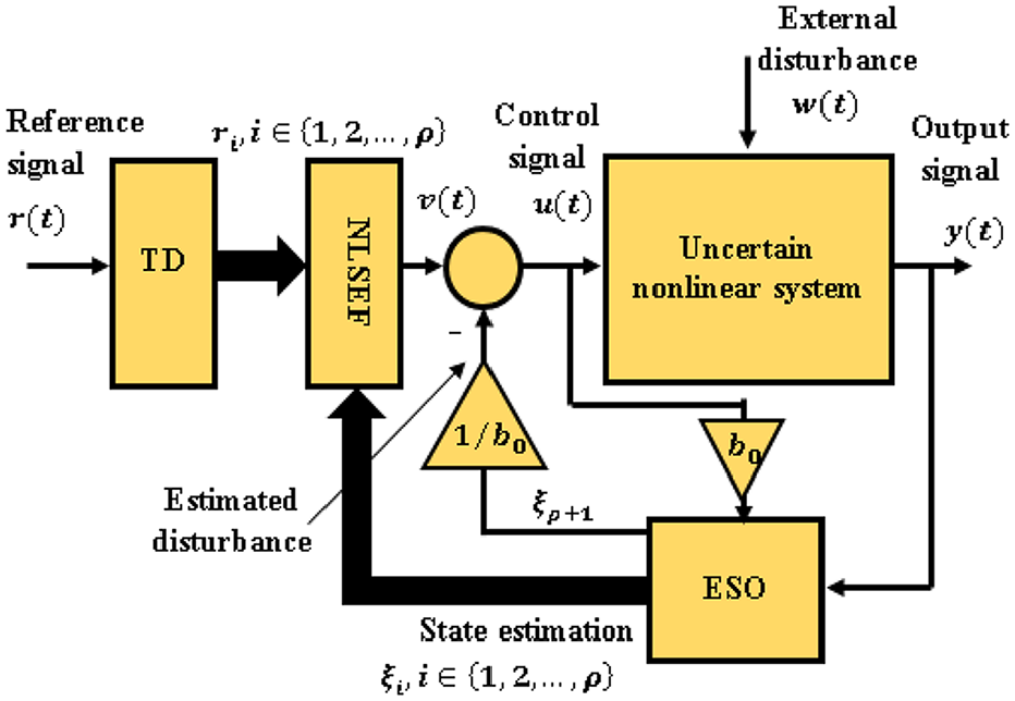
Active disturbance rejection control (ADRC) is an advanced robust control strategy, which works by augmenting the mathematical model of the nonlinear dynamical system with an additional virtual state. This virtual state describes all the unwanted dynamics, uncertainties, and exogenous disturbances, named as the “generalized disturbance” or “total disturbance.” This virtual state together with the states of the dynamic system is observed in real-time fashion using the extended state observer (ESO), which is the core part of the ADRC. It performs direct and active prediction and cancelation to the generalized disturbance by feeding back the estimated generalized disturbance into the input channel after simple manipulation. With ADRC, controlling a complex time-varying nonlinear system is transformed into a simple and linearized process. The superiority that makes it such a successful, robust control tool is that it is an error-driven technique, rather than model-based control law. Mainly, ADRC consists of an ESO, a tracking differentiator (TD), and a nonlinear state error combination (NLSEF) as illustrated in Figure 1,^27–29 where $r\in \mathbb{R}$ is the reference input, $(r_1{r}_2\dots r{)}^T\in {\mathbb{R}}^n$ is the transient profile, $v\in \mathbb{R}$ is the control input for the linearized model, $({\hat{\xi }}_1{\hat{\xi }}_2\dots {\hat{\xi }}_{n+1}{)}^T\in {\mathbb{R}}^{n+1}$ is the augmented estimated vector which comprises the plant states ${\hat{\xi }}_1,\dots ,{\hat{\xi }}_n$ and the estimated generalized disturbance ${\hat{\xi }}_{n+1}$ , which are produced by the ESO, and $b_0$ is the input gain.

Figure 1.

Structure of conventional ADRC.

Statement of contribution

The contribution of this paper lies in the following:

1. Proposing an AIOFL technique for a single-link flexible joint manipulator (SLFJM) which is a highly nonlinear uncertain system based on the IADRC with an improved nonlinear extended state observer (INLESO) of a saturation-like behavior developed in our previous work. ²⁹

2. We used the INLESO not only as an estimator for the system states $(x_1,\dots ,x_n)$ but also as a part of the linearization process where the generalized disturbance $(x_{n+1})$ is rejected from the input channel in an online manner as shown in Figure 1. The advantage of this technique is that it transforms any nonlinear uncertain system with exogenous disturbances and uncertainties into a pure chain of integrators up to the relative degree of the system. The proposed AIOFL method is effective due to its simplicity; for linearization, the only required information is the relative order of the system.

3. Another point of contribution is the stability investigation of the AIOFL achieved via the Lyapunov stability analysis for both linear extended state observer (LESO) and INLESO and the study of the asymptotic behavior of the closed-loop system using the Hurwitz stability theorem.

To the best of our knowledge, no previous research found in the literature that describes the linearization process for a nonlinear uncertain system within the context of ADRC with detailed stability analysis and extensive simulations on a highly nonlinear uncertain system. This paper is organized as follows. In section “Background and problem statement,” background and problem statement is introduced. In section “Proposed AIOFL,” the proposed AIOFL is discussed with detailed stability analysis and proofs. In section “Guideway example,” an SLFJM is presented as a guideway example for the proposed AIOFL method. Finally, the conclusions are drawn in section “Conclusion.”

Background and problem statement

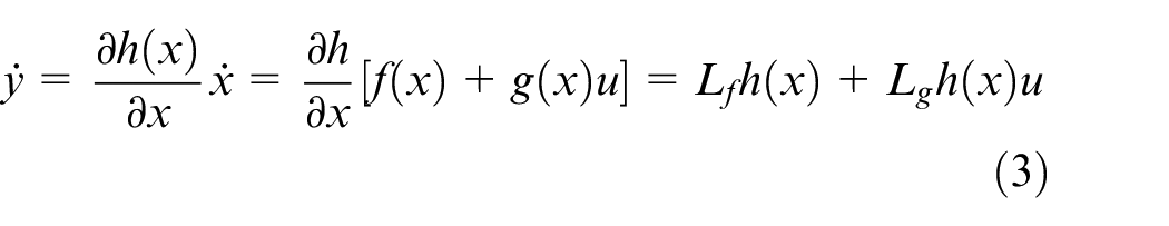
To perform IOFL, conditions have to be derived and stated which allow us to do the transformation to the nonlinear system such that the input–output map is linear. Given $\stackrel{·}{y}$ as

$$\stackrel{·}{y}=\frac{\partial h\left(x\right)}{\partial x}\stackrel{·}{x}=\frac{\partial h}{\partial x}[f\left(x\right)+g\left(x\right)u]=L_{f}h\left(x\right)+L_{g}h\left(x\right)u$$

(3)

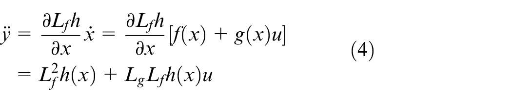
where $L_{f}h(x)=(\partial h/\partial x)f(x)$ is called the Lie derivative of $h(x)$ with respect to f. If $L_{g}h(x)=0$ , then $\stackrel{·}{y}=L_{f}h(x)$ is independent of u. The second derivative of y, denoted by $\widehat{y}$ , is given by

$$\begin{array}{c}\multicolumn{1}{c}{\stackrel{··}{y}=\frac{\partial L_{f}h}{\partial x}\stackrel{·}{x}=\frac{\partial L_{f}h}{\partial x}[f\left(x\right)+g\left(x\right)u]}\\ =L_f^{2}h\left(x\right)+L_g{L}_{f}h\left(x\right)u\hfill \end{array}$$

(4)

Once again, if $L_g{L}_{f}h(x)=0$ , then $y=L_f^{2}h(x)$ , which is also independent of u. Repeating this process with $h(x)$ , one gets

$$\{\begin{array}{c}{L}_g{L_f}^{i-1}h\left(x\right)=0,i=1,2,\dots ,\rho -1\hfill \\ \multicolumn{1}{c}{L_g{L_f}^{\rho -1}h\left(x\right)\ne 0}\end{array}$$

(5)

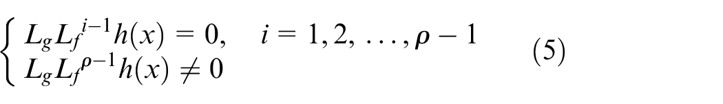
It can be seen that u is not included in $y,\stackrel{·}{y},\dots ,y^{(\rho -1)}$ but $y^{(\rho )}$ with a nonzero coefficient, $y^{(\rho )}={L_f}^{\rho }h(x)+L_g{L}_f^{\rho -1}h(x)u$ . The control signal $u=1/(L_g{L_f}^{\rho -1}h(x))[-{L_f}^{\rho }h(x)+v]$ reduces the input–output map to $y^{(\rho )}=v$ . Obviously, the system is input–output feedback linearizable, that is, the nonlinear system (1) is represented by a chain of integrators, where $\rho$ is denoted as the relative degree of the nonlinear system. Now let

$$z=T\left(x\right)=\left(\begin{array}{c}{\varphi }_1\left(x\right)\hfill \\ \multicolumn{1}{c}{⋮}\\ \multicolumn{1}{c}{\begin{array}{c}{\varphi }_{n-\rho }\left(x\right)\hfill \\ \multicolumn{1}{c}{\dots }\\ \multicolumn{1}{c}{\begin{array}{c}h\left(x\right)\hfill \\ \multicolumn{1}{c}{⋮}\\ \multicolumn{1}{c}{L_f^{\rho -1}h\left(x\right)}\end{array}}\end{array}}\end{array}\right)\underset{¯}{\underset{¯}{\mathrm{def}}}\left(\begin{array}{c}\varphi \left(x\right)\hfill \\ \multicolumn{1}{c}{\dots }\\ \multicolumn{1}{c}{\psi \left(x\right)}\end{array}\right)\underset{¯}{\underset{¯}{\mathrm{def}}}\left(\begin{array}{c}\eta \hfill \\ \multicolumn{1}{c}{\dots }\\ \multicolumn{1}{c}{\xi }\end{array}\right)$$

(6)

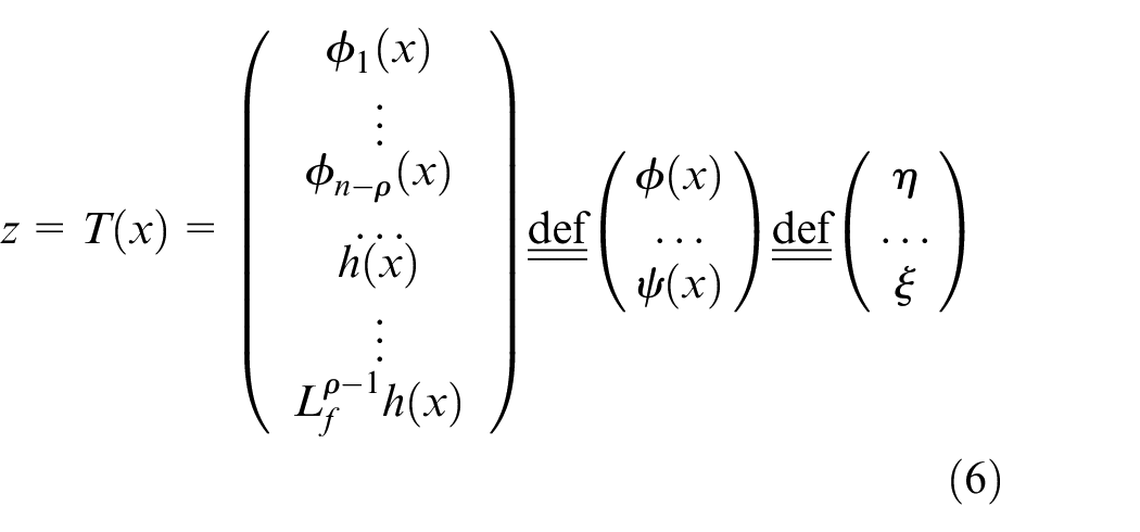
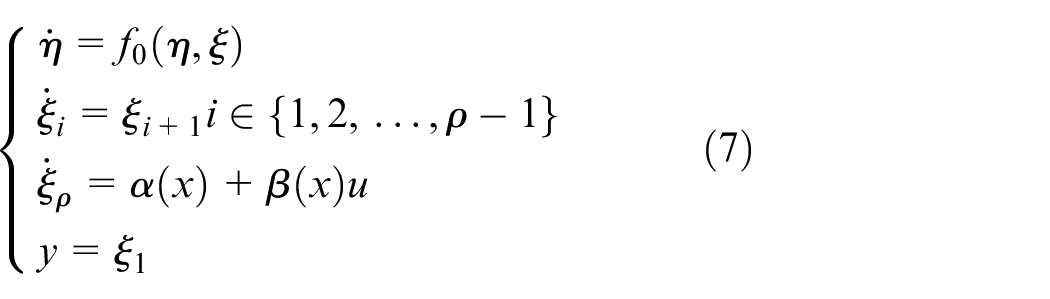
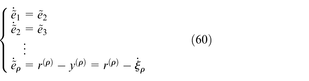
where ${\varphi }_1(x)$ to ${\varphi }_{n-\rho }(x)$ are chosen such that $(\partial {\varphi }_i(x)/\partial x)g(x)=0\mathrm{for}i\in \{1,2,\dots ,n-\rho \}\forall x\in D$ . This condition ensures that when the following equation is calculated $\stackrel{·}{\eta }=(\partial \varphi (x)/\partial x)[f(x)+g(x)u]=f_0(\eta .\xi )+g_0(\eta .\xi )u$ , the term u cancels out. It is now easy to verify that $z=T(x)$ transforms the system into normal form denoted as

$$\{\begin{array}{c}\stackrel{·}{\eta }=f_0(\eta ,\xi )\hfill \\ {\stackrel{·}{\xi }}_i={\xi }_{i+1}i\in \{1,2,\dots ,\rho -1\}\hfill \\ {\stackrel{·}{\xi }}_{\rho }=\alpha \left(x\right)+\beta \left(x\right)u\hfill \\ y={\xi }_1\hfill \end{array}$$

(7)

where $\alpha (x)={L_f}^{\rho }h(x)\mathrm{and}\beta (x)=L_g{L}_f^{\rho -1}h(x)$ . The internal dynamics are described by $\stackrel{·}{\eta }=f_0(\eta ,\xi )$ . The zero dynamics of the system are stated as $\stackrel{·}{\eta }=f_0(\eta ,\mathrm{\xi })$ with ξ = 0 $(\mathrm{i}.\mathrm{e}.\stackrel{·}{\eta }=f_0(\eta ,0))$ . The system is called minimum phase if the zero dynamics of the system are (globally) asymptotically stable.

Proposed AIOFL

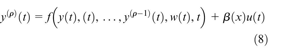
Consider the nonlinear single-input and single-output (SISO) system given as

$$y^{\left(\rho \right)}\left(t\right)=f(y\left(t\right),\left(t\right),\dots ,y^{(\rho -1)}\left(t\right),w\left(t\right),t)+\beta \left(x\right)u\left(t\right)$$

(8)

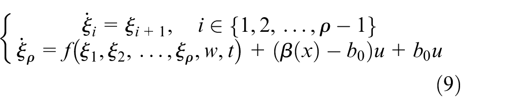
where $y^{(i)}(t)$ indicates ith derivative of y (the output), w and u represent the disturbance and the input, respectively, and $f\in \mathrm{C}({\mathbb{R}}^{\rho }\times \mathbb{R}\times \mathbb{R},\mathbb{R})$ is an uncertain function. Many classes of nonlinear systems can be represented in this notation, for example, time-varying or time-invariant systems and nonlinear or linear systems. For more straightforward representation and without causing any ambiguity, the time variable will be omitted from the equations. Assuming ${\xi }_1=y,{\xi }_2=\stackrel{·}{y},\dots ,{\xi }_{\rho }=y^{(\rho -1)}$ , one gets

$$\{\begin{array}{c}{\stackrel{·}{\xi }}_i={\xi }_{i+1},i\in \{1,2,\dots ,\rho -1\}\hfill \\ \multicolumn{1}{c}{{\stackrel{·}{\xi }}_{\rho }=f({\xi }_1,{\xi }_2,\dots ,{\xi }_{\rho },w,t)+(\beta \left(x\right)-b_0)u+b_{0}u}\end{array}$$

(9)

The above representation is sometimes called the Brunovsky form. Augmenting the system with the additional state, ${\xi }_{\rho +1}=f+(\beta (x)-b_0)u=f_T\Rightarrow {\stackrel{·}{\xi }}_{\rho +1}=\mathrm{\Delta }(t)={\stackrel{·}{f}}_T$ . The coefficient $b_0$ is a rough approximation of $\beta (x)$ in the plant within a ±50% range ¹⁴ and $f_T=f+(\beta (x)-b_0)u$ is the generalized disturbance, which consists of all of the unknown external disturbances, system uncertainties, and internal dynamics. The parameter $b_0$ usually chosen explicitly by the user as a design parameter.

LESO

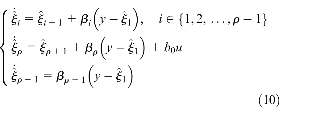
The states of the system in equation (9) together with the generalized disturbance $f_T$ will be estimated by an LESO, given by^30,31

$$\{\begin{array}{c}{\stackrel{·}{\hat{\xi }}}_i={\hat{\xi }}_{i+1}+{\beta }_i(y-{\hat{\xi }}_1),i\in \{1,2,\dots ,\rho -1\}\hfill \\ {\stackrel{·}{\hat{\xi }}}_{\rho }={\hat{\xi }}_{\rho +1}+{\beta }_{\rho }(y-{\hat{\xi }}_1)+b_{0}u\hfill \\ {\stackrel{·}{\hat{\xi }}}_{\rho +1}={\beta }_{\rho +1}(y-{\hat{\xi }}_1)\hfill \end{array}$$

(10)

where ${\hat{\xi }}_1,\dots ,{\hat{\xi }}_{\rho }$ are the estimated states up to the relative degree $\rho$ of system (9), ${\hat{\xi }}_{\rho +1}$ is the estimated generalized disturbance, and ${\beta }_{i}i\in \{1,2,\dots ,\rho +1\}$ are the LESO gains. The noteworthy feature of the basic LESO and its variants is that it needs minimum information about the dynamical system, and only the relative degree $\rho$ of the underlying system is needed to the design of the LESO. Several modifications have been developed to expand the basic features of the LESO to adapt to a broader class of dynamical systems. ³⁰ In this section, the convergence of the LESO and the INLESO is demonstrated using the Lyapunov analysis.

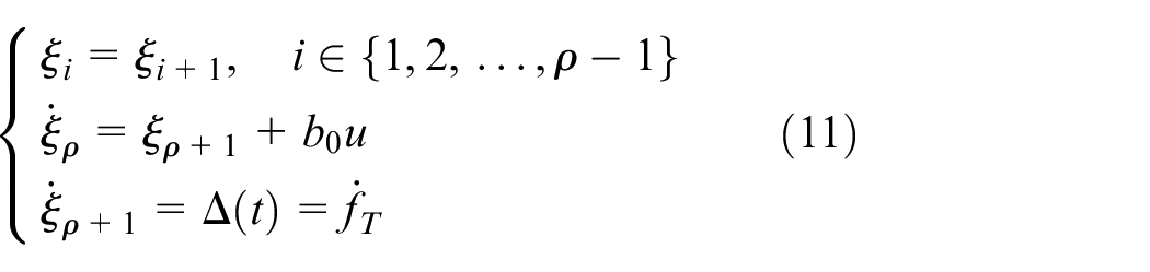
Consider system (9) with the augmented state ${\xi }_{\rho +1}$ is given as

$$\{\begin{array}{c}{\xi }_i={\xi }_{i+1},i\in \{1,2,\dots ,\rho -1\}\hfill \\ {\stackrel{·}{\xi }}_{\rho }={\xi }_{\rho +1}+b_{0}u\hfill \\ {\stackrel{·}{\xi }}_{\rho +1}=\mathrm{\Delta }\left(t\right)={\stackrel{·}{f}}_T\hfill \end{array}$$

(11)

Assumption (A1)

The function $f_T$ is continuously differentiable.

Assumption (A2)

There exists a positive constant M such that $|\mathrm{\Delta }(t)|\le M$ for $t\ge 0$ .

Assumption (A3)

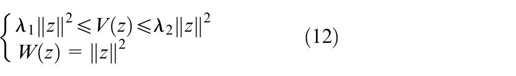
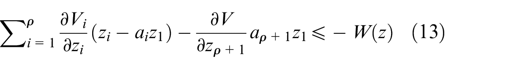
There exist constants ${\lambda }_1\mathrm{and}{\lambda }_2$ and positive definite, continuously differentiable functions $V,W:{\mathbb{R}}^{n+1}\to {\mathbb{R}}^{+}$ such that ³¹

$$\{\begin{array}{c}{\lambda }_1\Vert z{\Vert }^2\le V\left(z\right)\le {\lambda }_2\Vert z{\Vert }^2\hfill \\ \multicolumn{1}{c}{W\left(z\right)=\Vert z{\Vert }^2}\end{array}$$

(12)

$$\sum _{i=1}^{\rho }\frac{\partial V_i}{\partial z_i}(z_i-a_i{z}_1)-\frac{\partial V}{\partial z_{\rho +1}}{a}_{\rho +1}{z}_1\le -W\left(z\right)$$

(13)

Lemma 1 (LESO convergence)

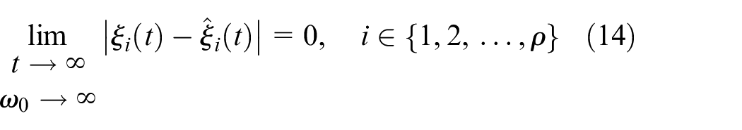
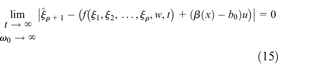
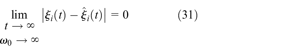
Given the nonlinear system expressed as in equation (11) and the LESO given in equation (10). If Assumptions (A1)–(A3) hold, then, for any initial values of the system states ${\xi }_i,i\in \{1,2,\dots ,\rho \}$ , the states of the LESO converge to that of the nonlinear system, that is

$$\underset{\begin{array}{c}t\to \infty \hfill \\ \multicolumn{1}{c}{{\omega }_0\to \infty }\end{array}}{lim}|{\xi }_i\left(t\right)-{\hat{\xi }}_i\left(t\right)|=0,i\in \{1,2,\dots ,\rho \}$$

(14)

$$\underset{\begin{array}{c}t\to \infty \hfill \\ \multicolumn{1}{c}{{\omega }_0\to \infty }\end{array}}{lim}|{\hat{\xi }}_{\rho +1}-(f({\xi }_1,{\xi }_2,\dots ,{\xi }_{\rho },w,t)+(\beta \left(x\right)-b_0)u)|=0$$

(15)

where ${\xi }_i(t)$ and ${\hat{\xi }}_i(t)$ denote the solutions of equations (11) and (10), respectively, where $i\in \{1,2,\dots ,\rho +1\}$ .

Proof

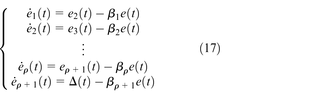
We make use of Guo et al. ³¹ to prove the convergence for the LESO. Set $e_i(t)={\xi }_i(t)-{\hat{\xi }}_i(t)$ , for $i\in \{1,2,\dots ,\rho +1\}$ . Then, subtracting equation (10) from equation (11), one gets

$$\{\begin{array}{c}{\stackrel{·}{\xi }}_1\left(t\right)-{\hat{\xi }}_1\left(t\right)={\xi }_2\left(t\right)-({\hat{\xi }}_2\left(t\right)+{\beta }_1(y\left(t\right)-{\hat{\xi }}_1\left(t\right)))\hfill \\ \multicolumn{1}{c}{{\stackrel{·}{\xi }}_2\left(t\right)-{\hat{\xi }}_2\left(t\right)={\xi }_3\left(t\right)-({\hat{\xi }}_3\left(t\right)+{\beta }_2(y\left(t\right)-{\hat{\xi }}_1\left(t\right)))}\\ \multicolumn{1}{c}{⋮}\\ \multicolumn{1}{c}{{\stackrel{·}{\xi }}_{\rho }\left(t\right)-{\stackrel{·}{\hat{\xi }}}_{\rho }\left(t\right)={\xi }_{\rho +1}\left(t\right)+b_{0}u\left(t\right)}\\ \multicolumn{1}{c}{-({\hat{\xi }}_{\rho +1}\left(t\right)+b_{0}u\left(t\right)+{\beta }_{\rho }(y\left(t\right)-{\hat{\xi }}_1\left(t\right)))}\\ \multicolumn{1}{c}{{\stackrel{·}{\xi }}_{\rho +1}\left(t\right)-{\hat{\xi }}_{\rho +1}\left(t\right)=\mathrm{\Delta }\left(t\right)-{\beta }_{\rho +1}(y\left(t\right)-{\hat{\xi }}_1\left(t\right))}\end{array}$$

(16)

Direct computations show that the estimated error dynamics satisfy

$$\{\begin{array}{c}{\stackrel{·}{e}}_1\left(t\right)=e_2\left(t\right)-{\beta }_{1}e\left(t\right)\hfill \\ \multicolumn{1}{c}{{\stackrel{·}{e}}_2\left(t\right)=e_3\left(t\right)-{\beta }_{2}e\left(t\right)}\\ \multicolumn{1}{c}{⋮}\\ \multicolumn{1}{c}{{\stackrel{·}{e}}_{\rho }\left(t\right)=e_{\rho +1}\left(t\right)-{\beta }_{\rho }e\left(t\right)}\\ \multicolumn{1}{c}{{\stackrel{·}{e}}_{\rho +1}\left(t\right)=\mathrm{\Delta }\left(t\right)-{\beta }_{\rho +1}e\left(t\right)}\end{array}$$

(17)

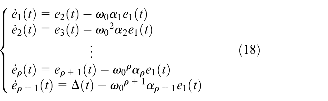
Let ${\beta }_i={\alpha }_i{{\omega }_0}^i$ , where ${\alpha }_i,i\in \{1,2,\dots ,\rho +1\}$ are the design gain parameters of the LESO associated with each ${{\omega }_0}^i$ , and ${\omega }_0$ is the bandwidth of the LESO. Expressing ${\beta }_i$ as ${\alpha }_i{{\omega }_0}^i$ , the system of equation (17) can be written as

$$\{\begin{array}{c}{\stackrel{·}{e}}_1\left(t\right)=e_2\left(t\right)-{\omega }_0{\alpha }_1{e}_1\left(t\right)\hfill \\ \multicolumn{1}{c}{{\stackrel{·}{e}}_2\left(t\right)=e_3\left(t\right)-{{\omega }_0}^2{\alpha }_2{e}_1\left(t\right)}\\ \multicolumn{1}{c}{⋮}\\ \multicolumn{1}{c}{{\stackrel{·}{e}}_{\rho }\left(t\right)=e_{\rho +1}\left(t\right)-{{\omega }_0}^{\rho }{\alpha }_{\rho }{e}_1\left(t\right)}\\ \multicolumn{1}{c}{{\stackrel{·}{e}}_{\rho +1}\left(t\right)=\mathrm{\Delta }\left(t\right)-{{\omega }_0}^{\rho +1}{\alpha }_{\rho +1}{e}_1\left(t\right)}\end{array}$$

(18)

Assuming ${\eta }_i(t)={{\omega }_0}^{\rho +1-i}{e}_i(t/{\omega }_0),i\in \{1,2,\dots ,\rho +1\}$ , then

$$e_i\left(\frac{t}{{\omega }_0}\right)=\frac{1}{{{\omega }_0}^{\rho +1-i}}{\eta }_i\left(t\right)$$

(19)

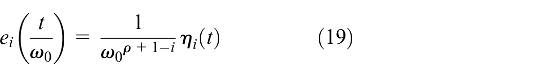
Then, time-scaled estimation error dynamics are expressed as

$$\{\begin{array}{c}\frac{d{\eta }_1\left(t\right)}{\mathrm{dt}}={\eta }_2\left(t\right)-{\alpha }_1{\eta }_1\left(t\right)\hfill \\ \frac{d{\eta }_2\left(t\right)}{\mathrm{dt}}={\eta }_3\left(t\right)-{\alpha }_2{\eta }_1\left(t\right)\hfill \\ ⋮\hfill \\ \frac{d{\eta }_{\rho }\left(t\right)}{\mathrm{dt}}={\eta }_{\rho +1}\left(t\right)-{\alpha }_n{\eta }_i\left(t\right)\hfill \\ \frac{d{\eta }_{\rho +1}\left(t\right)}{\mathrm{dt}}=\frac{\mathrm{\Delta }}{{\omega }_0}-{\alpha }_{\rho +1}{\eta }_1\left(t\right)\hfill \end{array}$$

(20)

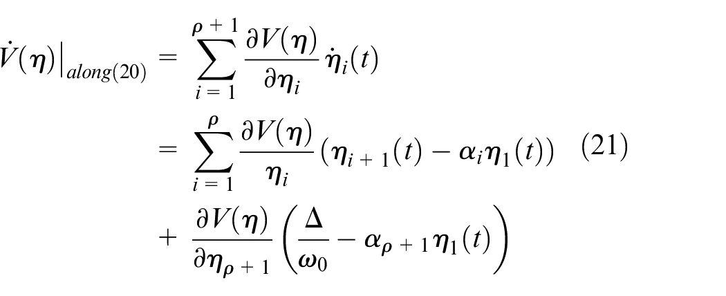
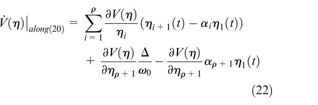
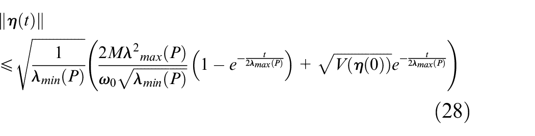
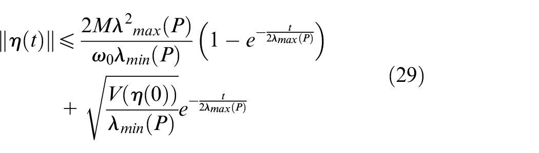
Assume the candidate Lyapunov functions $V,W:{\mathbb{R}}^{n+1}\to {\mathbb{R}}^{+}$ defined by $V(\eta )=<P\eta ,\eta >$ , where $\eta \in {\mathbb{R}}^{\rho +1}$ and P is a symmetric positive definite matrix. Suppose that in Assumption (A3) holds with ${\lambda }_1={\lambda }_{\min }(P)$ and ${\lambda }_2={\lambda }_{\max }(P)$ , where ${\lambda }_{\min }(P)$ and ${\lambda }_{\max }(P)$ are the minimal and maximal eigenvalues of P, respectively. Then, finding $\stackrel{·}{V}$ (the differentiation of $V(\eta )$ ) w.r.t. t over $\eta$ (solution (20)) is accomplished in the following way

$$\begin{array}{c}\multicolumn{1}{c}{{\stackrel{·}{V}\left(\eta \right)|}_{\mathrm{along}\left(20\right)}=\sum _{i=1}^{\rho +1}\frac{\partial V\left(\eta \right)}{\partial {\eta }_i}{\stackrel{·}{\eta }}_i\left(t\right)}\\ =\sum _{i=1}^{\rho }\frac{\partial V\left(\eta \right)}{{\eta }_i}({\eta }_{i+1}\left(t\right)-{\alpha }_i{\eta }_1\left(t\right))\hfill \\ +\frac{\partial V\left(\eta \right)}{\partial {\eta }_{\rho +1}}(\frac{\mathrm{\Delta }}{{\omega }_0}-{\alpha }_{\rho +1}{\eta }_1\left(t\right))\hfill \end{array}$$

(21)

Then

$$\begin{array}{c}\multicolumn{1}{c}{{\stackrel{·}{V}\left(\eta \right)|}_{\mathrm{along}\left(20\right)}=\sum _{i=1}^{\rho }\frac{\partial V\left(\eta \right)}{{\eta }_i}({\eta }_{i+1}\left(t\right)-{\alpha }_i{\eta }_1\left(t\right))}\\ +\frac{\partial V\left(\eta \right)}{\partial {\eta }_{\rho +1}}\frac{\mathrm{\Delta }}{{\omega }_0}-\frac{\partial V\left(\eta \right)}{\partial {\eta }_{\rho +1}}{\alpha }_{\rho +1}{\eta }_1\left(t\right)\hfill \end{array}$$

(22)

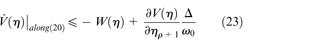
If the inequality equation (13) in Assumption (A3) is satisfied, then

$${\stackrel{·}{V}\left(\eta \right)|}_{\mathrm{along}\left(20\right)}\le -W\left(\eta \right)+\frac{\partial V\left(\eta \right)}{\partial {\eta }_{\rho +1}}\frac{\mathrm{\Delta }}{{\omega }_0}$$

(23)

Since $|\partial V/\partial {\eta }_{\rho +1}|\le ||\partial V(\eta )/\partial \eta ||$ and $V(\eta )\le {\lambda }_{\max }(P)||\eta |{|}^2$ , one can obtain $|\partial V/\partial {\eta }_{\rho +1}|\le 2{\lambda }_{\max }(P)||\eta ||$ . Moreover, since ${\lambda }_{\min }(P)||\eta |{|}^2\le V(\eta )$ , this leads to $||\eta ||\le \sqrt{V(\eta )/{\lambda }_{\min }(P)}$ . This results in

$$\left|\frac{\partial V}{\partial {\eta }_{\rho +1}}\right|\le 2{\lambda }_{\max }\left(P\right)\sqrt{\frac{V\left(\eta \right)}{{\lambda }_{\min }\left(P\right)}}$$

(24)

Given that $V(\eta )\le {\lambda }_{\max }(P)||\eta |{|}^2={\lambda }_{\max }(P)W(\eta )$ , then

$$-W\left(\eta \right)\le \frac{-V\left(\eta \right)}{{\lambda }_{\max }\left(P\right)}$$

(25)

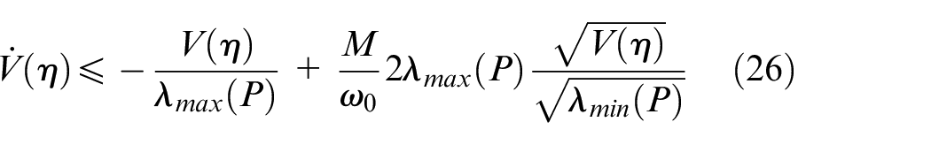
Given that the rate of change $\mathrm{\Delta }(t)$ of the generalized disturbance $f_T$ is bounded, namely, Assumption (A2) is fulfilled and substituting equations (24) and (25) in equation (23), we get

$$\stackrel{·}{V}\left(\eta \right)\le -\frac{V\left(\eta \right)}{{\lambda }_{\max }\left(P\right)}+\frac{M}{{\omega }_0}2{\lambda }_{\max }\left(P\right)\frac{\sqrt{V\left(\eta \right)}}{\sqrt{{\lambda }_{\min }\left(P\right)}}$$

(26)

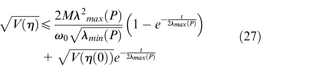
Knowing that $d/\mathrm{dt}\sqrt{V(\eta )}=(1/2)(1/\sqrt{V(\eta )})\stackrel{·}{V}(\eta )$ , then equation (26) is an ordinary first-order differential equation (26), and its solution can be found as

$$\begin{array}{c}\multicolumn{1}{c}{\sqrt{V\left(\eta \right)}\le \frac{2M{{\lambda }^2}_{\max }\left(P\right)}{{\omega }_0\sqrt{{\lambda }_{\min }\left(P\right)}}(1-e^{-\frac{t}{2{\lambda }_{\max }\left(P\right)}})}\\ +\sqrt{V\left(\eta \left(0\right)\right)}{e}^{-\frac{t}{2{\lambda }_{\max }\left(P\right)}}\hfill \end{array}$$

(27)

From Assumption (A3), ${\lambda }_{\min }(P)||\eta |{|}^2\le V(\eta )$ , this leads to $||\eta ||\le \sqrt{V(\eta )/{\lambda }_{\min }(P)}$ , then

$$\begin{array}{c}\Vert \eta \left(t\right)\Vert \hfill \\ \le \sqrt{\frac{1}{{\lambda }_{\min }\left(P\right)}}(\frac{2M{{\lambda }^2}_{\max }\left(P\right)}{{\omega }_0\sqrt{{\lambda }_{\min }\left(P\right)}}(1-e^{-\frac{t}{2{\lambda }_{\max }\left(P\right)}})+\sqrt{V\left(\eta \left(0\right)\right)}{e}^{-\frac{t}{2{\lambda }_{\max }\left(P\right)}})\hfill \end{array}$$

(28)

$$\begin{array}{c}\multicolumn{1}{c}{\Vert \eta \left(t\right)\Vert \le \frac{2M{{\lambda }^2}_{\max }\left(P\right)}{{\omega }_0{\lambda }_{\min }\left(P\right)}(1-e^{-\frac{t}{2{\lambda }_{\max }\left(P\right)}})}\\ +\sqrt{\frac{V\left(\eta \left(0\right)\right)}{{\lambda }_{\min }\left(P\right)}}{e}^{-\frac{t}{2{\lambda }_{\max }\left(P\right)}}\hfill \end{array}$$

(29)

It follows from equation (19) that

$$\begin{array}{c}|{\xi }_i\left(t\right)-{\hat{\xi }}_i\left(t\right)|=\frac{1}{{{\omega }_0}^{\rho +1-i}}\left|{\eta }_i\left({\omega }_{0}t\right)\right|\Rightarrow |{\xi }_i\left(t\right)-{\hat{\xi }}_i\left(t\right)|\hfill \\ \le \frac{1}{{{\omega }_0}^{\rho +1-i}}\Vert \eta \left(t\right)\Vert \hfill \end{array}$$

Then, equation (29) becomes

$$\begin{array}{c}|{\xi }_i\left(t\right)-{\hat{\xi }}_i\left(t\right)|\le \frac{1}{{{\omega }_0}^{\rho +1-i}}\hfill \\ (\frac{2M{{\lambda }^2}_{\max }\left(P\right)}{{\omega }_0{\lambda }_{\min }\left(P\right)}(1-e^{-\frac{t}{2{\lambda }_{\max }\left(P\right)}})+\sqrt{\frac{V\left(\eta \left(0\right)\right)}{{\lambda }_{\min }\left(P\right)}}{e}^{-\frac{t}{2{\lambda }_{\max }\left(P\right)}})\hfill \end{array}$$

(30)

Finally

$$\underset{\begin{array}{c}t\to \infty \hfill \\ \multicolumn{1}{c}{{\omega }_0\to \infty }\end{array}}{lim}|{\xi }_i\left(t\right)-{\hat{\xi }}_i\left(t\right)|=0$$

(31)

$$\underset{\begin{array}{c}t\to \infty \hfill \\ \multicolumn{1}{c}{{\omega }_0\to \infty }\end{array}}{lim}|{\hat{\xi }}_{\rho +1}-(f({\xi }_1,{\xi }_2,\dots ,{\xi }_{\rho },w,t)+(\beta \left(x\right)-b_0)u)|=0$$

(32)

▪

INLESO

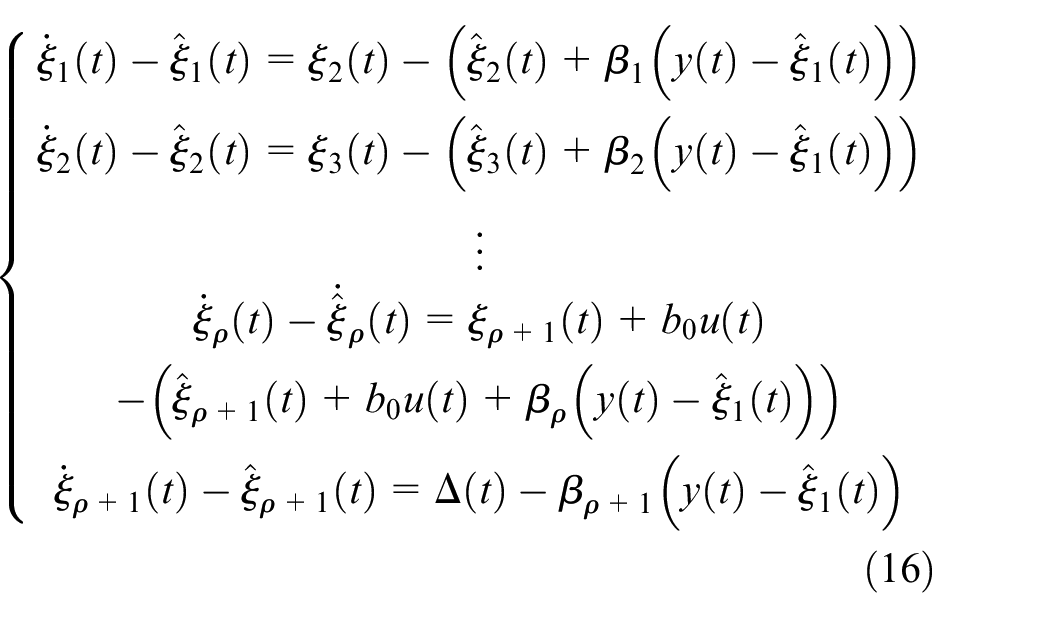
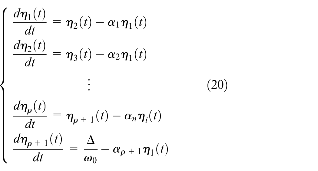
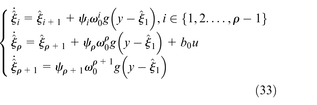
In the previous section, the application of LESO on the system of equation (9) and its convergence have been analyzed. In this section, the states of the system in equation (9) together with the generalized disturbance $f_T$ will be estimated by the INLESO given by

$$\{\begin{array}{c}{\stackrel{·}{\hat{\xi }}}_i={\hat{\xi }}_{i+1}+{\psi }_i{\omega }_0^{i}g(y-{\hat{\xi }}_1),i\in \{1,2.\dots ,\rho -1\}\hfill \\ \multicolumn{1}{c}{{\stackrel{·}{\hat{\xi }}}_{\rho }={\hat{\xi }}_{\rho +1}+{\psi }_{\rho }{\omega }_0^{\rho }g(y-{\hat{\xi }}_1)+b_{0}u}\\ \multicolumn{1}{c}{{\stackrel{·}{\hat{\xi }}}_{\rho +1}={\psi }_{\rho +1}{\omega }_0^{\rho +1}g(y-{\hat{\xi }}_1)}\end{array}$$

(33)

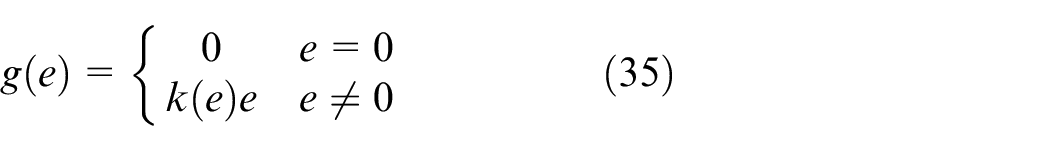
where ${\hat{\xi }}_1,\dots ,{\hat{\xi }}_{\rho }$ are the estimated states up to the relative degree $\rho$ of system (9), ${\hat{\xi }}_{\rho +1}$ is the estimated generalized disturbance, ${\psi }_{i}i\in \{1,2,\dots ,\rho +1\}$ are the INLESO gains, and ${\omega }_0$ is the INLESO bandwidth. The nonlinear function $g:\mathbb{R}\to \mathbb{R}$ is designed as

$$g\left(e\right)=K_{\alpha }{\left|e\right|}^{{\alpha }_f}\mathrm{sign}\left(e\right)+K_{\beta }{\left|e\right|}^{\beta }e$$

(34)

where $K_{\alpha },K_{\beta },{\alpha }_f,\mathrm{and}\beta$ are the positive design parameters, and e is defined as $e=y-{\hat{\xi }}_1$ .

Remark 1

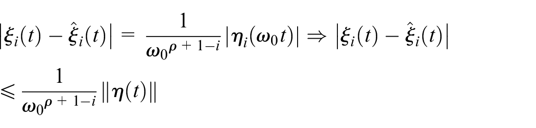
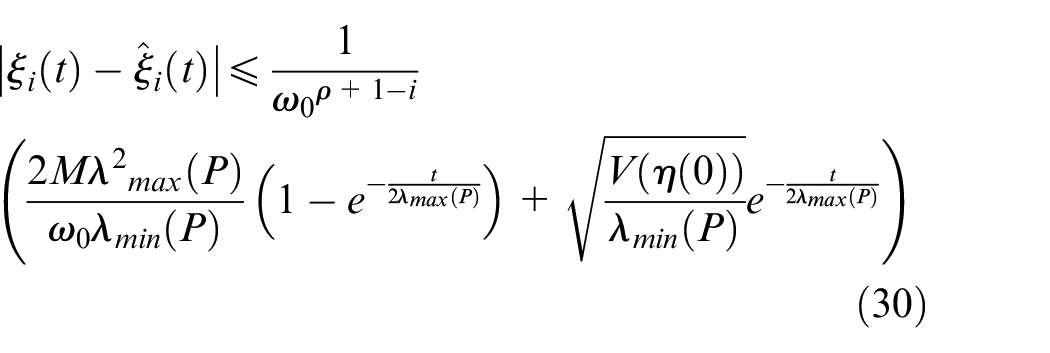
It is worthy to remember that in our work, we have assumed that the dynamics of the plant $\mathrm{\Delta }(t)={\stackrel{·}{f}}_T$ in equation (11) are mostly unknown. Consequently, the steady-state observer estimation errors $e_i(t)={\xi }_i(t)-{\hat{\xi }}_i(t)$ for $i\in \{1,2,\dots ,\rho +1\}$ are bounded, and their upper bound is monotonically shrinking with the bandwidth of the observer as evident from equation (30). Then, as $e_i(t)\to 0$ in equation (30), the closed-loop system would satisfy the Lipschitz condition, the stability analysis with the Lyapunov function is still valid, and $g(e)$ in equation (34) does not exhibit any numerical problems whatever the values of ${\alpha }_f$ and $\beta$ are.

Since $\mathrm{sign}(e)=e/|e|$ , for $|e|\ne 0$ , then

$$g\left(e\right)=\{\begin{array}{cc}0\hfill & e=0\hfill \\ \multicolumn{1}{c}{k\left(e\right)e}& e\ne 0\hfill \end{array}$$

(35)

The function $k:\mathbb{R}/\{0\}\to {\mathbb{R}}^{+}$ is an even nonlinear gain function with $k(e)=K_{\alpha }|e{|}^{{\alpha }_f-1}+K_{\beta }|e{|}^{\beta }$ . The convergence of the INLESO will be investigated in Lemma 2; before that, the following assumption is needed.

Assumption 4 (A4)

There exist constants ${\lambda }_1\mathrm{and}{\lambda }_2$ and positive definite, continuously differentiable functions $V,W:{\mathbb{R}}^{n+1}\to {\mathbb{R}}^{+}$ such that

$${\lambda }_1\Vert z{\Vert }^2\le V\left(z\right)\le {\lambda }_2\Vert z{\Vert }^2$$

(36)

$$W\left(z\right)=\Vert z{\Vert }^2$$

(37)

$$\begin{array}{c}\sum _{i=1}^{\rho }\frac{\partial V_i}{\partial z_i}(z_i-a_{i}k\left(\frac{z_1}{{{\omega }_0}^{\rho }}\right)z_1)\hfill \\ -\frac{\partial V}{\partial z_{\rho +1}}{a}_{\rho +1}k\left(\frac{z_1}{{{\omega }_0}^{\rho }}\right)z_1\le -W\left(z\right)\hfill \end{array}$$

(38)

Lemma 2 (convergence of the INLESO)

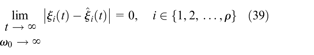
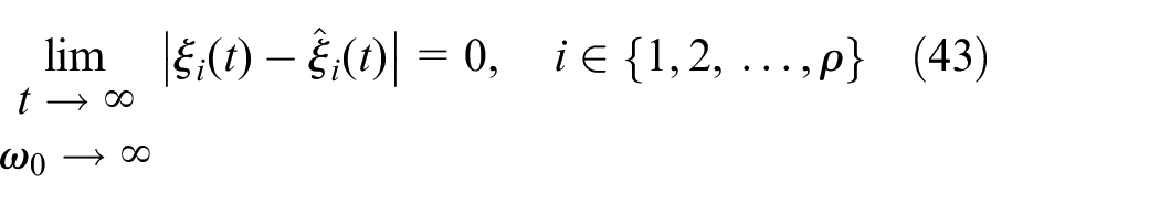
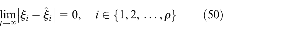
Given the system set out in equation (9) and the INLESO equation (33), it follows that under Assumptions A1, A2, and A4, for any initial values of the system states ${\xi }_i,i\in \{1,2,\dots ,\rho \}$

$$\underset{\begin{array}{c}t\to \infty \hfill \\ \multicolumn{1}{c}{{\omega }_0\to \infty }\end{array}}{lim}|{\xi }_i\left(t\right)-{\hat{\xi }}_i\left(t\right)|=0,i\in \{1,2,\dots ,\rho \}$$

(39)

$$\underset{t\to \infty }{lim}|{\hat{\xi }}_{\rho +1}-(f({\xi }_1,{\xi }_2,\dots ,{\xi }_{\rho },w,t)+(\beta \left(x\right)-b_0)u)|=0$$

(40)

where ${\xi }_i$ and ${\hat{\xi }}_i$ denote the solutions of equations (9) and (33), respectively, where $i\in \{1,2,\dots ,\rho +1\}$ .

Proof

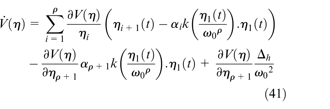
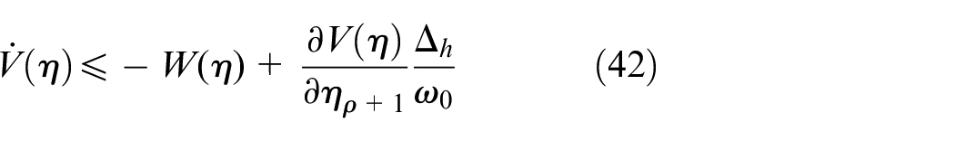
Following the same steps of the proof of Lemma 1 with Assumptions A1 and A2, we get the following

$$\begin{array}{c}\multicolumn{1}{c}{\stackrel{·}{V}\left(\eta \right)=\sum _{i=1}^{\rho }\frac{\partial V\left(\eta \right)}{{\eta }_i}({\eta }_{i+1}\left(t\right)-{\alpha }_{i}k\left(\frac{{\eta }_1\left(t\right)}{{{\omega }_0}^{\rho }}\right).{\eta }_1\left(t\right))}\\ -\frac{\partial V\left(\eta \right)}{\partial {\eta }_{\rho +1}}{\alpha }_{\rho +1}k\left(\frac{{\eta }_1\left(t\right)}{{{\omega }_0}^{\rho }}\right).{\eta }_1\left(t\right)+\frac{\partial V\left(\eta \right)}{\partial {\eta }_{\rho +1}}\frac{{\mathrm{\Delta }}_h}{{{\omega }_0}^2}\hfill \end{array}$$

(41)

If Assumption A4 is satisfied, then

$$\stackrel{·}{V}\left(\eta \right)\le -W(\eta )+\frac{\partial V\left(\eta \right)}{\partial {\eta }_{\rho +1}}\frac{{\mathrm{\Delta }}_h}{{\omega }_0}$$

(42)

Substituting equations (24) and (25) in equation (42), we reach to equation (26). Moreover, solving equation (26) with simple manipulations on its solutions (27) as done in the proof of Lemma 1, we get

$$\underset{\begin{array}{c}t\to \infty \hfill \\ \multicolumn{1}{c}{{\omega }_0\to \infty }\end{array}}{lim}|{\xi }_i(t)-{\hat{\xi }}_i(t)|=0,i\in \{1,2,\dots ,\rho \}$$

(43)

$$\underset{t\to \infty }{lim}|{\hat{\xi }}_{\rho +1}-(f({\xi }_1,{\xi }_2,\dots ,{\xi }_{\rho },w,t)+(\beta \left(x\right)-b_0)u)|=0$$

(44)

▪

Theorem 1 (AIOFL)

Given the nonlinear system of equation (11) and the LESO or INLESO in equations (10) or (33), respectively. Then, the nonlinear system of equation (9) or (11) is reduced to a chain of integrators described as

$${\xi }_i={\xi }_{i+1},i\in \{1,2,\dots ,\rho -1\}$$

(45)

$${\stackrel{·}{\xi }}_{\rho }=b_{0}v$$

(46)

Proof

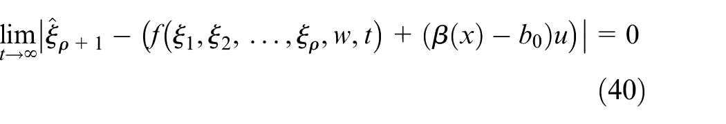
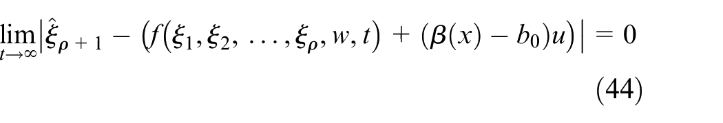
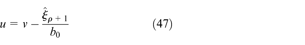
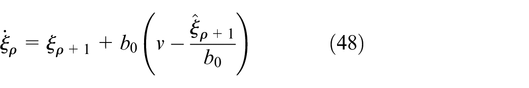
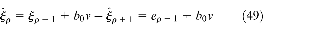
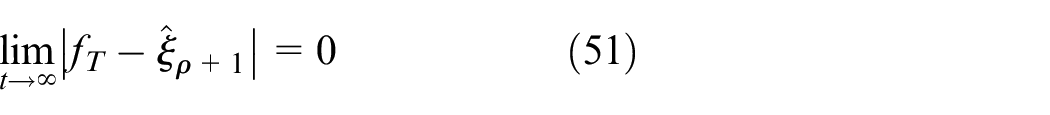
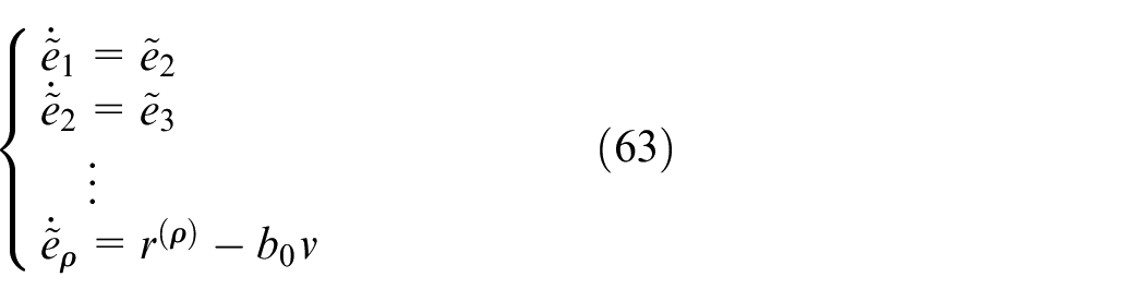
Based on the result of Lemma 1 and Lemma 2 and if the LCL u is selected as

$$u=v-\frac{{\hat{\xi }}_{\rho +1}}{b_0}$$

(47)

then

$${\stackrel{·}{\xi }}_{\rho }={\xi }_{\rho +1}+b_0(v-\frac{{\hat{\xi }}_{\rho +1}}{b_0})$$

(48)

$${\stackrel{·}{\xi }}_{\rho }={\xi }_{\rho +1}+b_{0}v-{\hat{\xi }}_{\rho +1}=e_{\rho +1}+b_{0}v$$

(49)

${\stackrel{·}{\xi }}_{\rho }\approx b_{0}v$ (for large ${\omega }_0$ ).▪

Remark 2

The main differences between IOFL and AIOFL are, for the AIOFL, there is no need to obtain the transformation of equation (6). The only required information is the relative degree of the system $(\rho )$ for the nonlinear system to be linearized. While, for the IOFL, transformation equation (6) is the key step to linearize the system. It is based on the exact mathematical cancelation of the nonlinear terms $\alpha (x)$ and $\beta (x)$ , which requires knowledge of $\alpha$ , $\beta$ , and T. Furthermore, AIOFL in addition to linearizing the nonlinear system, it lumps the external disturbances, uncertainties, and unmodeled dynamics into a single term for online and active estimation and cancelation later on.

Stability of the closed-loop system

The stability of the closed-loop system with the IADRC is considered in the following. Before that, the following assumptions are needed.

Assumption 5 (A5)

The states ${\xi }_i(i=1,2,\dots ,\rho )$ and the generalized disturbance f of an n-dimensional uncertain nonlinear SISO system (9) are estimated by a convergent LESO which produces the estimated states ${\hat{\xi }}_i(i=1,2,\dots ,\rho )$ of the plant and the estimated generalized disturbance ${\hat{\xi }}_{\rho +1}$ as $t\to \infty$ , respectively, that is

$$\underset{t\to \infty }{lim}|{\xi }_i-{\hat{\xi }}_i|=0,i\in \{1,2,\dots ,\rho \}$$

(50)

and

$$\underset{t\to \infty }{lim}|f_T-{\hat{\xi }}_{\rho +1}|=0$$

(51)

Assumption 6 (A6)

A TD produces a trajectory $r_i,i\in \{1,2,\dots ,\rho \}$ with minimum setpoint change. The trajectory converges to a reference trajectory $r^{(i-1)}\mathrm{for}i\in \{1,2,\dots ,\rho \}$ as $t\to \infty$ , that is

$$\underset{t\to \infty }{lim}|r^{(i-1)}-r_i|=0,i\in \{1,2,\dots ,\rho \}$$

(52)

Theorem 2 (closed-loop stability)

Consider an n-dimensional uncertain nonlinear SISO system given in equation (9). System (9) is controlled by the LCL u given by

$$u=v-\frac{{\hat{\xi }}_{\rho +1}}{b_0}$$

(53)

where v is given as

$$v=k_1\left({\tilde{e}}_1\right){\tilde{e}}_1+k_2\left({\tilde{e}}_2\right){\tilde{e}}_2+\cdots +k_n\left({\tilde{e}}_n\right){\tilde{e}}_n$$

(54)

where $k_i:\mathbb{R}\to {\mathbb{R}}^{+}$ is an even nonlinear gain function and ${\tilde{e}}_i=r_i-{\hat{x}}_i,i\in \{1,2,\dots ,\rho \}$ is the tracking error. Assuming that Assumptions A5 and A6 hold, then, the closed-loop system is asymptotically stable, that is, $\underset{t\to \infty }{lim}|{\tilde{e}}_i|=0,i\in \{1,2,\dots ,\rho \}$ .

Proof

The tracking error between the reference trajectory and the corresponding plant estimated states is given as

$${\tilde{e}}_i=r_i-{\hat{\xi }}_i,i\in \{1,2,\dots ,\rho \}$$

(55)

With LESO and TD as in Assumptions A4 and A5, respectively, the tracking error can be described as

$${\tilde{e}}_i=r^{(i-1)}-{\xi }_i,i\in \{1,2,\dots ,\rho \}$$

(56)

For the system given in equation (9), the states ${\xi }_i$ are expressed in terms of the plant output

$${\xi }_i=y^{(i-1)},i\in \{1,2,\dots ,\rho \}$$

(57)

Substitute equation (57) in equation (56) and the tracking error is given by

$${\tilde{e}}_i=r^{(i-1)}-y^{(i-1)},i\in \{1,2,\dots ,\rho \}$$

(58)

Differentiating equation (58) w.r.t. t gives

$${\stackrel{·}{\stackrel{~}{e}}}_i=r^{\left(i\right)}-y^{\left(i\right)}={\tilde{e}}_{i+1},i\in \{1,2,\dots ,\rho \}$$

(59)

It follows that the tracking error dynamics ${\tilde{e}}_i,i\in \{1,2,\dots ,\rho \}$ are given below

$$\{\begin{array}{c}{\stackrel{·}{\stackrel{~}{e}}}_1={\tilde{e}}_2\hfill \\ \multicolumn{1}{c}{{\stackrel{·}{\stackrel{~}{e}}}_2={\tilde{e}}_3}\\ \multicolumn{1}{c}{⋮}\\ \multicolumn{1}{c}{{\stackrel{·}{\stackrel{~}{e}}}_{\rho }=r^{\left(\rho \right)}-y^{\left(\rho \right)}=r^{\left(\rho \right)}-{\stackrel{·}{\xi }}_{\rho }}\end{array}$$

(60)

This together with equation (9) gives

$$\{\begin{array}{c}{\stackrel{·}{\stackrel{~}{e}}}_1={\tilde{e}}_2\hfill \\ \multicolumn{1}{c}{{\stackrel{·}{\stackrel{~}{e}}}_2={\tilde{e}}_3}\\ \multicolumn{1}{c}{⋮}\\ \multicolumn{1}{c}{{\stackrel{·}{\stackrel{~}{e}}}_{\rho }=r^{\left(\rho \right)}-(f_T+b_{0}u)}\end{array}$$

(61)

Substituting equation (53) in equation (61) results in

$$\{\begin{array}{c}{\stackrel{·}{\stackrel{~}{e}}}_1={\tilde{e}}_2\hfill \\ \multicolumn{1}{c}{{\stackrel{·}{\stackrel{~}{e}}}_2={\tilde{e}}_3}\\ \multicolumn{1}{c}{⋮}\\ \multicolumn{1}{c}{{\stackrel{·}{\stackrel{~}{e}}}_{\rho }=r^{\left(\rho \right)}-b_{0}v+{\hat{\xi }}_{\rho +1}-f_T}\end{array}$$

(62)

It follows from equations (51) and (57) that

$$\{\begin{array}{c}{\stackrel{·}{\stackrel{~}{e}}}_1={\tilde{e}}_2\hfill \\ \multicolumn{1}{c}{{\stackrel{·}{\stackrel{~}{e}}}_2={\tilde{e}}_3}\\ \multicolumn{1}{c}{⋮}\\ \multicolumn{1}{c}{{\stackrel{·}{\stackrel{~}{e}}}_{\rho }=r^{\left(\rho \right)}-b_{0}v}\end{array}$$

(63)

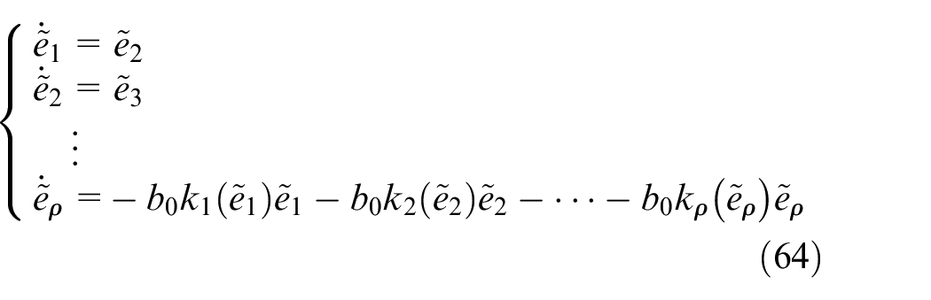
The tracking error dynamics given in equation (63) associated with the control law v designed in equation (54) produce the following closed-loop tracking error dynamics

$$\{\begin{array}{c}{\stackrel{·}{\stackrel{~}{e}}}_1={\tilde{e}}_2\hfill \\ \multicolumn{1}{c}{{\stackrel{·}{\stackrel{~}{e}}}_2={\tilde{e}}_3}\\ \multicolumn{1}{c}{⋮}\\ \multicolumn{1}{c}{{\stackrel{·}{\stackrel{~}{e}}}_{\rho }=-b_0{k}_1\left({\tilde{e}}_1\right){\tilde{e}}_1-b_0{k}_2\left({\tilde{e}}_2\right){\tilde{e}}_2-\cdots -b_0{k}_{\rho }\left({\tilde{e}}_{\rho }\right){\tilde{e}}_{\rho }}\end{array}$$

(64)

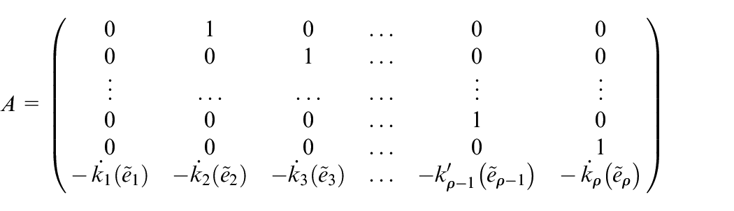
The dynamics given in equation (64) can be represented as

$${\stackrel{·}{\stackrel{~}{e}}}^{=}A\tilde{e}$$

(65)

where

$$A=\left(\begin{array}{cccccc}0\hfill & 1\hfill & 0\hfill & \dots \hfill & 0\hfill & 0\hfill \\ \multicolumn{1}{c}{0}& 0\hfill & 1\hfill & \dots \hfill & 0\hfill & 0\hfill \\ \multicolumn{1}{c}{⋮}& \dots \hfill & \dots \hfill & \dots \hfill & ⋮\hfill & ⋮\hfill \\ \multicolumn{1}{c}{0}& 0\hfill & 0\hfill & \dots \hfill & 1\hfill & 0\hfill \\ \multicolumn{1}{c}{0}& 0\hfill & 0\hfill & \dots \hfill & 0\hfill & 1\hfill \\ \multicolumn{1}{c}{-{\stackrel{·}{k}}_1\left({\tilde{e}}_1\right)}& -{\stackrel{·}{k}}_2\left({\tilde{e}}_2\right)\hfill & -{\stackrel{·}{k}}_3\left({\tilde{e}}_3\right)\hfill & \dots \hfill & -k{\prime }_{\rho -1}\left({\tilde{e}}_{\rho -1}\right)\hfill & -{\stackrel{·}{k}}_{\rho }\left({\tilde{e}}_{\rho }\right)\hfill \end{array}\right)$$

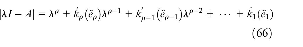
and $\tilde{e}=({\tilde{e}}_1,{\tilde{e}}_2,\dots ,{\tilde{e}}_{\rho }{)}^T$ and $({\stackrel{·}{k}}_i{\tilde{e}}_i)=b_0{k}_i({\tilde{e}}_i),i\in \{1,2,\dots ,\rho \}$ . The characteristic polynomial of A is given by

$$|\lambda I-A|={\lambda }^{\rho }+{\stackrel{·}{k}}_{\rho }\left({\tilde{e}}_{\rho }\right){\lambda }^{\rho -1}+k_{\rho -1}^{\prime }\left({\tilde{e}}_{\rho -1}\right){\lambda }^{\rho -2}+\cdots +{\stackrel{·}{k}}_1\left({\tilde{e}}_1\right)$$

(66)

The design parameters of $({\stackrel{·}{k}}_i{\tilde{e}}_i)$ are selected to ensure that the roots of the characteristic polynomial equation (66) have strictly negative real parts, that is, the Hurwitz (stable) polynomial.▪

Guideway example

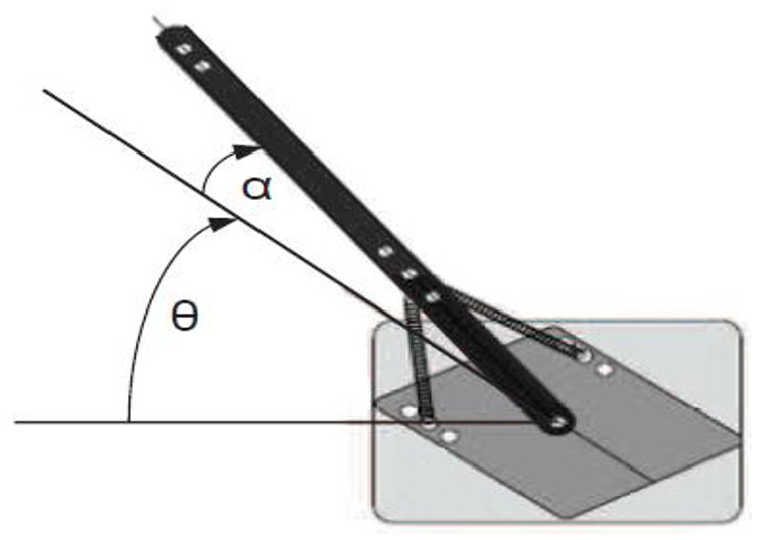
In this example, an SISO SLFJM offered by Groves and Serrani ³² is studied and shown in Figure 2.

Figure 2.

Definition of generalized coordinates for the SLFJM.

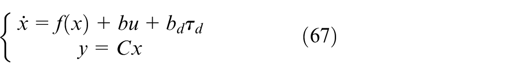
The state-space representation of the SLFJM system in the form of the nonlinear system given in equation (1) is described as

$$\{\begin{array}{c}\stackrel{·}{x}=f\left(x\right)+\mathrm{bu}+b_d{\tau }_d\hfill \\ \multicolumn{1}{c}{y=\mathrm{Cx}}\end{array}$$

(67)

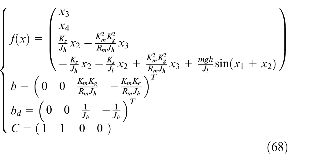
where $x=(x_1{x}_2{x}_3{x}_4{)}^T=(\theta \alpha \stackrel{·}{\theta }\stackrel{·}{\alpha }{)}^T\in {\mathbb{R}}^4$ is the plant state, $u\in \mathbb{R}$ is the plant input, ${\tau }_d\in \mathbb{R}$ is the exogenous disturbance, $y=(\theta +\alpha )\in \mathbb{R}$ is the plant output, $f:{\mathbb{R}}^4\to \mathbb{R}$ , $\theta$ is the motor angular displacement, and $\alpha$ is the joint twist or link deflection. The components of $f,b,b_d,C$ are denoted, respectively, by

$$\{\begin{array}{c}f\left(x\right)=\left(\begin{array}{c}{x}_3\hfill \\ \multicolumn{1}{c}{x_4}\\ \multicolumn{1}{c}{\frac{K_s}{J_h}{x}_2-\frac{K_m^2{K}_g^2}{R_m{J}_h}{x}_3}\\ \multicolumn{1}{c}{-\frac{K_s}{J_h}{x}_2-\frac{K_s}{J_l}{x}_2+\frac{K_m^2{K}_g^2}{R_m{J}_h}{x}_3+\frac{\mathrm{mgh}}{J_l}\sin (x_1+x_2)}\end{array}\right)\hfill \\ \multicolumn{1}{c}{b={\left(\begin{array}{cccc}0\hfill & 0\hfill & \frac{K_m{K}_g}{R_m{J}_h}\hfill & -\frac{K_m{K}_g}{R_m{J}_h}\hfill \end{array}\right)}^T}\\ \multicolumn{1}{c}{b_d={\left(\begin{array}{cccc}0\hfill & 0\hfill & \frac{1}{J_h}\hfill & -\frac{1}{J_h}\hfill \end{array}\right)}^T}\\ \multicolumn{1}{c}{C=\left(\begin{array}{ccc}1\hfill & 1\hfill & \begin{array}{cc}0\hfill & 0\hfill \end{array}\hfill \end{array}\right)}\end{array}$$

(68)

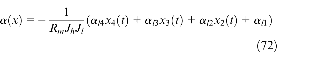
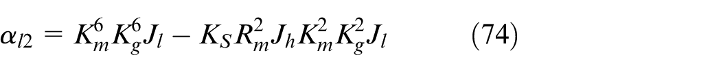
where $K_s$ is the link stiffness, $J_h$ is the inertia of hub, m is the link mass, h is the height of hub, $K_m$ is the motor constant, $K_g$ is the gear ratio, $J_l$ is the load inertia, and $R_m$ is the motor resistance. The values of the coefficients for SLFJM are: ³² $K_s=1.61$ , $J_h=0.0021$ , $m=0.403$ , $g=-9.81$ , $h=0.06$ , $K_m=0.00767$ , $K_g=70$ , $J_i={0.0059}^T$ , and $R_m=2.6$ . Applying the Lie derivative on equation (68), we get the following set of equations ³³

$$L_{g}h\left(x\right)=0,L_g{L_f}^{1}h\left(x\right)=0$$

(69)

$$L_g{L_f}^{2}h\left(x\right)=0,L_g{L_f}^{3}h\left(x\right)\ne 0$$

(70)

It can be noticed that the SLFJM system in equation (68) satisfies equation (5); consequently, the relative order of SLFJM is 4, that is, $\rho =4$ . ³³ Three control configurations have been considered for linearization in this work and applied on SLFJM; they are explained in the next with their simulation results.

Traditional IOFL transformation

The IOFL is given as

$$v=\alpha \left(x\right)+\beta \left(x\right)u$$

(71)

such that $u={\beta }^{-1}(x)(v-\alpha (x))$ . In this method, we assume that the system states are available for feedback with no need for state observer. Thus

$$\alpha \left(x\right)=-\frac{1}{R_m{J}_h{J}_l}({\alpha }_{l4}{x}_4\left(t\right)+{\alpha }_{l3}{x}_3\left(t\right)+{\alpha }_{l2}{x}_2\left(t\right)+{\alpha }_{l1})$$

(72)

$${\alpha }_{l1}=-K_s{R}_m^3{J}_h^2\mathrm{mgh}\sin (x_1\left(t\right)+x_3\left(t\right))$$

(73)

$${\alpha }_{l2}=K_m^6{K}_g^6{J}_l-K_S{R}_m^2{J}_h{K}_m^2{K}_g^2{J}_l$$

(74)

$${\alpha }_{l3}=-K_m^4{K}_g^4{J}_l{K}_s{R}_m+K_s^2{R}_m^3{J}_h{J}_h+K_s^2{R}_m^3{J}_h^2$$

(75)

$${\alpha }_{l4}=K_S{R}_m^2{J}_h{K}_m^2{K}_g^2{J}_l$$

(76)

and

$$\beta \left(x\right)=\frac{k_m^5{K}_g^5}{R_m^3{J}_h^3}-\frac{K_m{K}_g{K}_s}{R_m{J}_h^2}$$

(77)

The linear control law v, which is taken as the standard linear PID controller, is given as

$$v=k_{p}e+k_d\frac{\mathrm{de}}{\mathrm{dt}}+k_i\int e\mathrm{dt}$$

(78)

Conventional active disturbance rejection control–based AIOFL

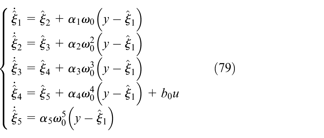
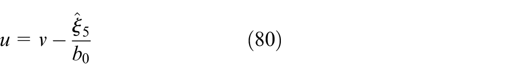
The conventional active disturbance rejection control (CADRC) is the combination of the LESO given by equation (79), the NLSEF given by equation (80), and TD given by equation (82). According to Aguilar-Ibañez et al. ³⁰ and Guo et al., ³¹ an LESO observer can be designed as

$$\{\begin{array}{c}{\stackrel{·}{\hat{\xi }}}_1={\hat{\xi }}_2+{\alpha }_1{\omega }_0(y-{\hat{\xi }}_1)\hfill \\ \multicolumn{1}{c}{{\stackrel{·}{\hat{\xi }}}_2={\hat{\xi }}_3+{\alpha }_2{\omega }_0^2(y-{\hat{\xi }}_1)}\\ \multicolumn{1}{c}{{\stackrel{·}{\hat{\xi }}}_3={\hat{\xi }}_4+{\alpha }_3{\omega }_0^3(y-{\hat{\xi }}_1)}\\ \multicolumn{1}{c}{{\stackrel{·}{\hat{\xi }}}_4={\hat{\xi }}_5+{\alpha }_4{\omega }_0^4(y-{\hat{\xi }}_1)+b_{0}u}\\ \multicolumn{1}{c}{{\stackrel{·}{\hat{\xi }}}_5={\alpha }_5{\omega }_0^5(y-{\hat{\xi }}_1)}\end{array}$$

(79)

where $\hat{\xi }=({\hat{\xi }}_1{\hat{\xi }}_2{\hat{\xi }}_3{\hat{\xi }}_4{)}^T$ is the vector of the estimated states of system (68), ${\hat{\xi }}_5$ is the estimated generalized disturbance, ${\alpha }_1,{\alpha }_2,{\alpha }_3,{\alpha }_4,\mathrm{and}{\alpha }_5$ are the LESO gains, and ${\omega }_0$ is the LESO bandwidth. The control law for the AIOFL is given as

$$u=v-\frac{{\hat{\xi }}_5}{b_0}$$

(80)

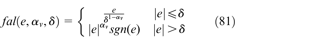
The linearized control law v is proposed as $v=\mathrm{fal}(e_1,{\alpha }_{v1},{\delta }_1)+\mathrm{fal}(e_2,{\alpha }_{v2},{\delta }_2)$ , with $\mathrm{fal}(.)$ defined as ²⁷

$$\mathrm{fal}(e,{\alpha }_v,\delta )=\{\begin{array}{cc}\frac{e}{{\delta }^{1-{\alpha }_v}}\hfill & \left|e\right|\le \delta \hfill \\ \multicolumn{1}{c}{{\left|e\right|}^{{\alpha }_v}\mathrm{sgn}(e)}& \left|e\right|>\delta \hfill \end{array}$$

(81)

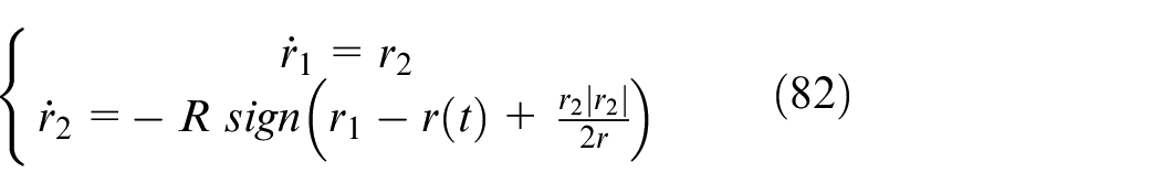
where $e=(e_1{e}_2{)}^T$ is the closed-loop tracking error vector which can be defined as $e_i=r_i-{\hat{\xi }}_i$ , i = 1, 2, and ${\alpha }_v\mathrm{and}\delta$ are the design parameters. The conventional second-order differentiator is given as ²⁷

$$\{\begin{array}{c}{\stackrel{·}{r}}_1=r_2\hfill \\ \multicolumn{1}{c}{{\stackrel{·}{r}}_2=-R\mathrm{sign}(r_1-r\left(t\right)+\frac{r_2\left|r_2\right|}{2r})}\end{array}$$

(82)

where r₁ is the tracking signal of the input r, and r₂ is the tracking signal of the derivative of the input r. To speed up or slow down the system during the transient, the coefficient R is adapted according to this, and it is an application dependent.

IADRC-based AIOFL

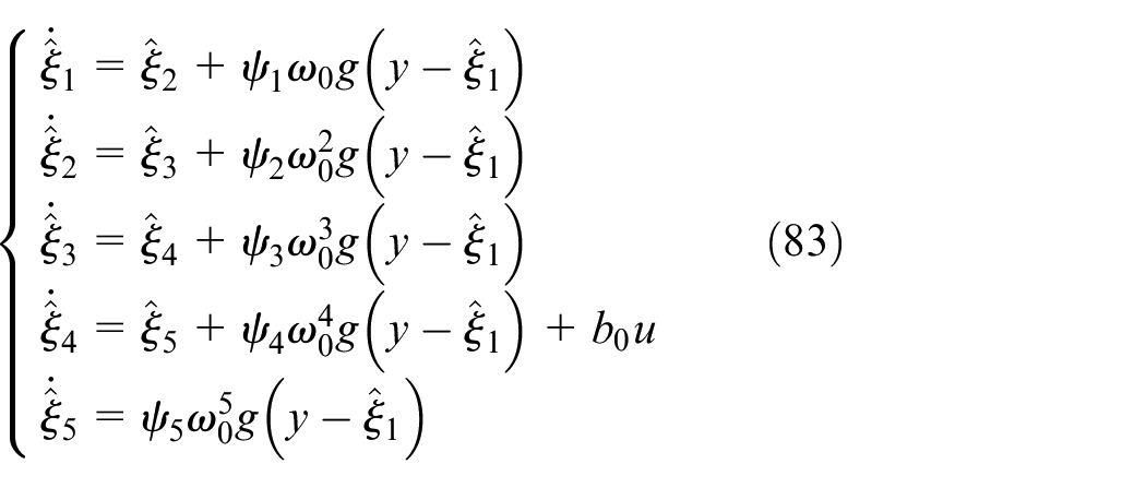
The IADRC has been designed in our previous works,^29,34,35 and tested on the differential drive mobile robot model ³⁶ and on permanent magnet direct current (PMDC) motor.^37,38 It is structured from the INLESO given by equation (83), ²⁹ the improved nonlinear state error feedback (INLSEF) given by equation (53), ³⁴ and the improved tracking differentiator (ITD) given by equation (89). ³⁵ The INLESO is the second type of observers used in these numerical simulations. The INLESO is described as

$$\{\begin{array}{c}{\stackrel{·}{\hat{\xi }}}_1={\hat{\xi }}_2+{\psi }_1{\omega }_{0}g(y-{\hat{\xi }}_1)\hfill \\ \multicolumn{1}{c}{{\stackrel{·}{\hat{\xi }}}_2={\hat{\xi }}_3+{\psi }_2{\omega }_0^{2}g(y-{\hat{\xi }}_1)}\\ \multicolumn{1}{c}{{\stackrel{·}{\hat{\xi }}}_3={\hat{\xi }}_4+{\psi }_3{\omega }_0^{3}g(y-{\hat{\xi }}_1)}\\ \multicolumn{1}{c}{{\stackrel{·}{\hat{\xi }}}_4={\hat{\xi }}_5+{\psi }_4{\omega }_0^{4}g(y-{\hat{\xi }}_1)+b_{0}u}\\ \multicolumn{1}{c}{{\stackrel{·}{\hat{\xi }}}_5={\psi }_5{\omega }_0^{5}g(y-{\hat{\xi }}_1)}\end{array}$$

(83)

where ${\psi }_1,{\psi }_2,{\psi }_3,{\psi }_4,\mathrm{and}{\psi }_5$ are the INLESO gains, and ${\omega }_0$ is the INLESO bandwidth. The nonlinear function $g(e):\mathbb{R}\to \mathbb{R}$ is designed as

$$g\left(e\right)=k_{\alpha }{\left|e\right|}^{{\alpha }_f}\mathrm{sign}\left(e\right)+k_{\beta }{\left|e\right|}^{\beta }e$$

(84)

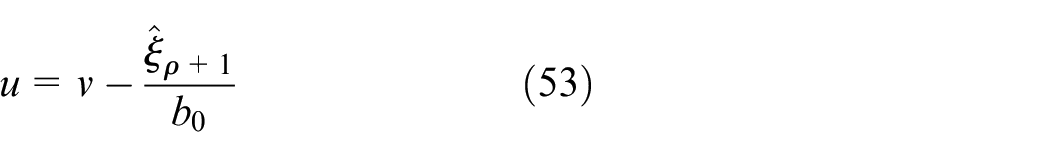
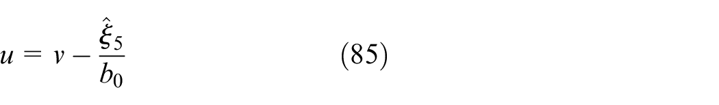
The control law for the AIOFL is defined as

$$u=v-\frac{{\hat{\xi }}_5}{b_0}$$

(85)

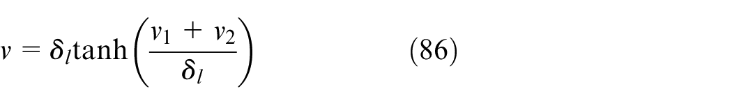
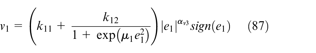
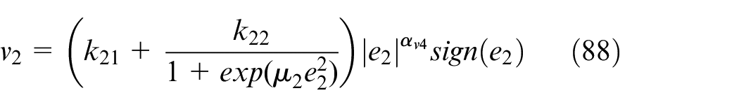
where v is the INLSEF given in our previous work as ³⁴

$$v={\delta }_l\tanh \left(\frac{v_1+v_2}{{\delta }_l}\right)$$

(86)

$$v_1=(k_{11}+\frac{k_{12}}{1+\exp \left({\mu }_1{e}_1^2\right)}){\left|e_1\right|}^{{\alpha }_{v3}}\mathrm{sign}\left(e_1\right)$$

(87)

$$v_2=(k_{21}+\frac{k_{22}}{1+\exp ({\mu }_2{e}_2^2)}){\left|e_2\right|}^{{\alpha }_{v4}}\mathrm{sign}\left(e_2\right)$$

(88)

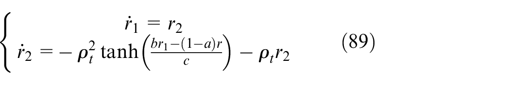
where $k_{11}$ , $k_{12}$ , ${\mu }_1$ , ${\alpha }_{v3}$ , $k_{21}$ , $k_{22}$ , ${\mu }_2$ , ${\alpha }_{v4}$ , and ${\delta }_l$ are the design parameters of the INLSEF controller. The third part of the IADRC is the ITD, and it is described as ³⁵

$$\{\begin{array}{c}{\stackrel{·}{r}}_1=r_2\hfill \\ \multicolumn{1}{c}{{\stackrel{·}{r}}_2=-{\rho }_t^2\tanh \left(\frac{b{r}_1-(1-a)r}{c}\right)-{\rho }_t{r}_2}\end{array}$$

(89)

where the coefficients $a,b,c,\mathrm{and}\rho$ are the suitable design coefficients with $0<a<1,b>0,c>0,\mathrm{and}{\rho }_t>0$ .

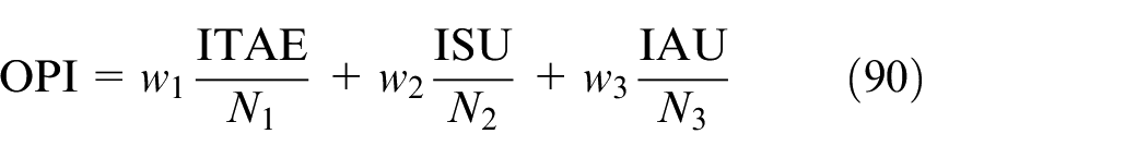
The AIOFL based on the classical LESO and INLESO is applied on the SLFJM given in equation (68). An objective performance index (OPI) is proposed to evaluate the performance of the LESO and the INLESO observers, which is represented as

$$\mathrm{OPI}=w_1\frac{\mathrm{ITAE}}{N_1}+w_2\frac{\mathrm{ISU}}{N_2}+w_3\frac{\mathrm{IAU}}{N_3}$$

(90)

where $\mathrm{ITAE}={\int }_0^{t_f}t|y-r|\mathrm{dt}$ is the integration of the time absolute error for the output signal, $\mathrm{ISU}={\int }_0^{t_f}{u}_o^2\mathrm{dt}$ is the integration of square of the control signal, and $\mathrm{IAU}={\int }_0^{t_f}\left|u_o\right|\mathrm{dt}$ is the integration of the absolute of the control signal. The weights must satisfy $w_1+w_2+w_3=1$ , and they are defined as the relative emphasis of one objective as compared to the other. The values of $w_1$ , $w_2$ , and $w_3$ are chosen to increase the pressure on the selected objective functions. The coefficients $N_1$ , $N_2$ , and $N_3$ are included in the performance index to ensure that the individual objectives have comparable values, and are treated equally likely by the tuning algorithm. Because, if a particular objective is of very high value, while the second one has shallow value, then the tuning algorithm will pay much consideration to the highest one and leave the other with little reflection on the system.

Simulation results

The tuning process for all the aforementioned three control schemes is achieved using the genetic algorithm (GA) with the OPI as the performance index as defined in equation (90) under MATLAB environment with $w_1=0.6$ , $w_2=0.2,w_3=0.6$ , $N_1=10$ , $N_2=2,N_3=2.7,$ and $t_f=6\mathrm{s}$ . Based on this, the parameters of the control law u for traditional IOFL control scheme are $k_p=18,369.94$ , $k_d=3.45$ , $k_i=1,824,382.96$ , ${\alpha }_{l1}=6.2163\times {10}^{-8}\sin (x_1(t)+x_3(t))$ , ${\alpha }_{l2}=0.0001,{\alpha }_{l3}=-0.0014$ , and ${\alpha }_{l4}=4.2758\times {10}^{-5}$ . While the values of the tuned parameters for the CADRC are—LESO: ${\omega }_0=513.8283$ , ${\alpha }_1=8.772$ , ${\alpha }_2=0.1946$ , ${\alpha }_3=0.7384$ , ${\alpha }_4=9.6881\times {10}^{-3}$ , ${\alpha }_5=2.2651\times {10}^{-6}$ , and $b_0=22.771$ ; TD: $R=2408.6918$ ; and NLSEF: ${\delta }_1=16.6108$ , ${\delta }_2=14.6238$ , ${\alpha }_{v1}=0.3804$ , and ${\alpha }_{v2}=0.4583$ . The values of tuned parameters for the IADRC are—INLESO: ${\omega }_0=104.6131$ , ${\psi }_1=0.1364$ , ${\psi }_2=0.6691$ , ${\psi }_3=0.6893$ , ${\psi }_4=0.0155$ , ${\psi }_5=14.3801\times {10}^{-6}$ , $b_0=8.74500$ , ${\alpha }_f=0.6906$ , $\beta =0.1880$ , $k_{\alpha }=0.3682$ , and $k_{\beta }=0.1290$ ; ITD: $a=0.9153$ , $b=8.7141$ , $c=0.0813$ , and ${\rho }_t=22.89333$ ; and INLSEF: $k_{11}=1.7741$ , $k_{12}=1.2147$ , $k_{21}=0.00115$ , $k_{22}=0.3312$ , ${\delta }_l=3.3900$ , ${\mu }_1=3.8297$ , ${\mu }_2=10.9415$ , ${\alpha }_{v3}=0.8244$ , and ${\alpha }_{v4}=1.8079$ .

It is worthy to note that in the AIOFL, the nonlinear system is linearized by either LESO or INLESO and represented by a chain of integrators. In this case, the LESO or INLESO will estimate the states of the chain of integrators up to the relative degree of the nonlinear system. With this arrangement, the higher-order estimated states represent signals with higher derivative degrees; they contain high-frequency components, which in turn increase the control signal activity and lead to the chattering phenomena. Based on the above reasoning, only the first two estimated states $({\hat{\xi }}_1\mathrm{and}{\hat{\xi }}_2)$ are fed back to either NLSEF or INLSEF in the numerical simulations. The entire estimated states of the system (except the augmented state) can be provided for feedback to the NLSEF. In our case, with the first two estimated states, it was sufficient to produce the individual control laws $(v_1\mathrm{and}{v}_2)$ which in turn generated the required control law $(v)$ . With this scenario, eliminating the states from the feedback that do not affect the performance of the system will reduce the number of the parameters of both the NLSEF controller and the TD. We expect that the total energy required for the controller to produce the control law $(v)$ will be reduced. The Runge–Kutta ODE45 solver in the MATLAB environment has been used for the numerical simulations of the continuous models. Three different scenarios are conducted in this work; they are as follows.

Reference tracking scenario

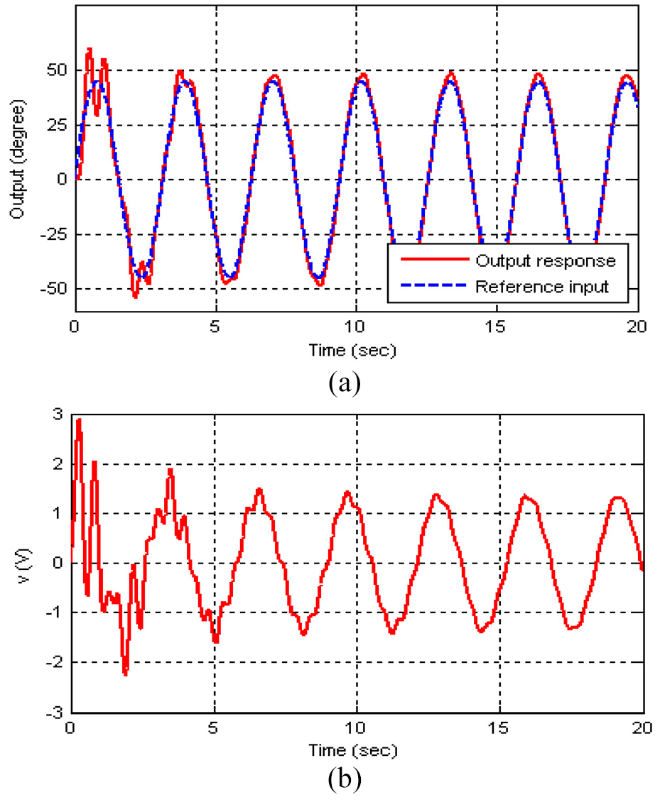
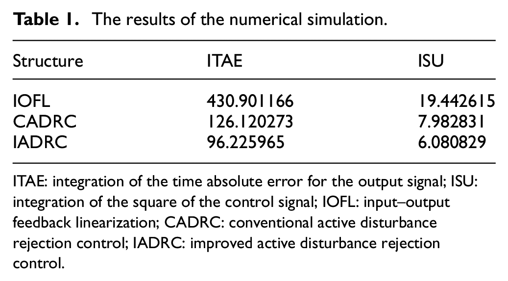
In this scenario, a sinusoidal signal with frequency 2 rad/s and amplitude of 45 has been chosen as a reference input. The simulation time is selected to be 20 s. The results of the numerical simulation are shown in Figures 3–5. The results are collected based on evaluating two indices listed in Table 1, where $\mathrm{ITAE}={\int }_0^{20}t|y-r|\mathrm{dt}$ is the integration of the time absolute error for the output signal, and $\mathrm{ISU}={\int }_0^{20}{u}^2\mathrm{dt}$ is the integration of the square of the control signal. The simulations show that the ISU index, which represents the energy delivered to the SLFJM motor, has been decreased by 23.82% and a noticeable improvement in the transient response (ITAE is reduced by 23.7%).

Figure 3.

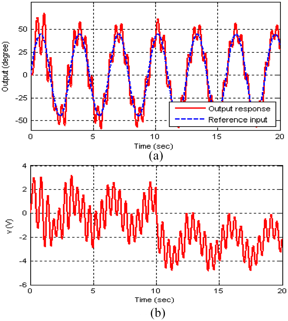
The curves of the numerical simulations for the first scenario using IOFL: (a) the output response of the SLFJM, y and (b) the control signal, v.

Figure 4.

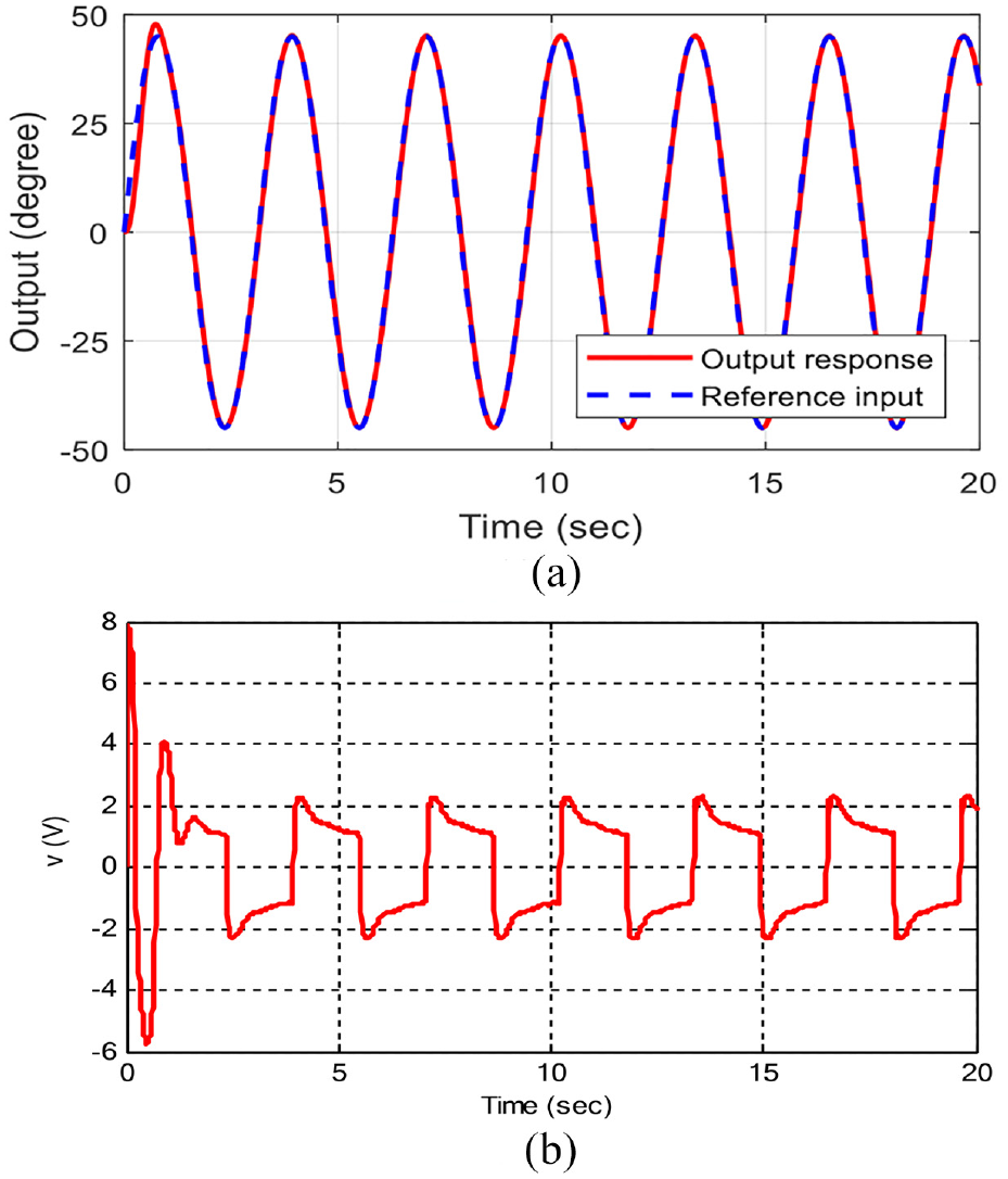
The curves of the numerical simulations for the first scenario using CADRC: (a) the output response of the SLFJM, y and (b) the control signal, v.

Figure 5.

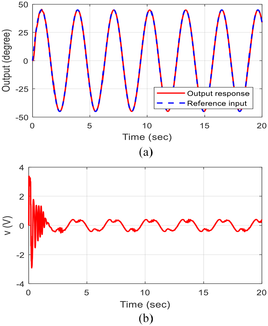
The curves of the numerical simulations for the first scenario using IADRC: (a) the output response of the SLFJM, y and (b) the control signal, v.

Table 1.

The results of the numerical simulation.

Structure	ITAE	ISU
IOFL	430.901166	19.442615
CADRC	126.120273	7.982831
IADRC	96.225965	6.080829

ITAE: integration of the time absolute error for the output signal; ISU: integration of the square of the control signal; IOFL: input–output feedback linearization; CADRC: conventional active disturbance rejection control; IADRC: improved active disturbance rejection control.

In this scenario, we can notice that the improvement of the accuracy of the reference tracking in the case of CADRC and IADRC as compared to the conventional IOFL, see Figures 3–5. The reason is due to the effectiveness of the ADRC as a robust tracking tool. Moreover, the control signal v produced by the IADRC (Figure 5(b)) is less chattering than that produced by the CADRC (Figure 4(b)) where the control signal v suffers from the peaking phenomenon due to the large values of the gain parameters of the LESO. The reason of the IADRC superiority is that the proposed nonlinear state error feedback of the IADRC produces the most economical control signal v satisfying the rule “small error, large gain and large error, small gain.” As listed in Table 1, there is a significant reduction in the delivered controller energy; this is evident from Figure 5(b) as compared to the control signal illustrated in Figures 3(b) and 4(b). Moreover, a noticeable reduction in the control energy using the IADRC technique is obvious in Table 1.

Inertia uncertainty and exogenous disturbance scenario

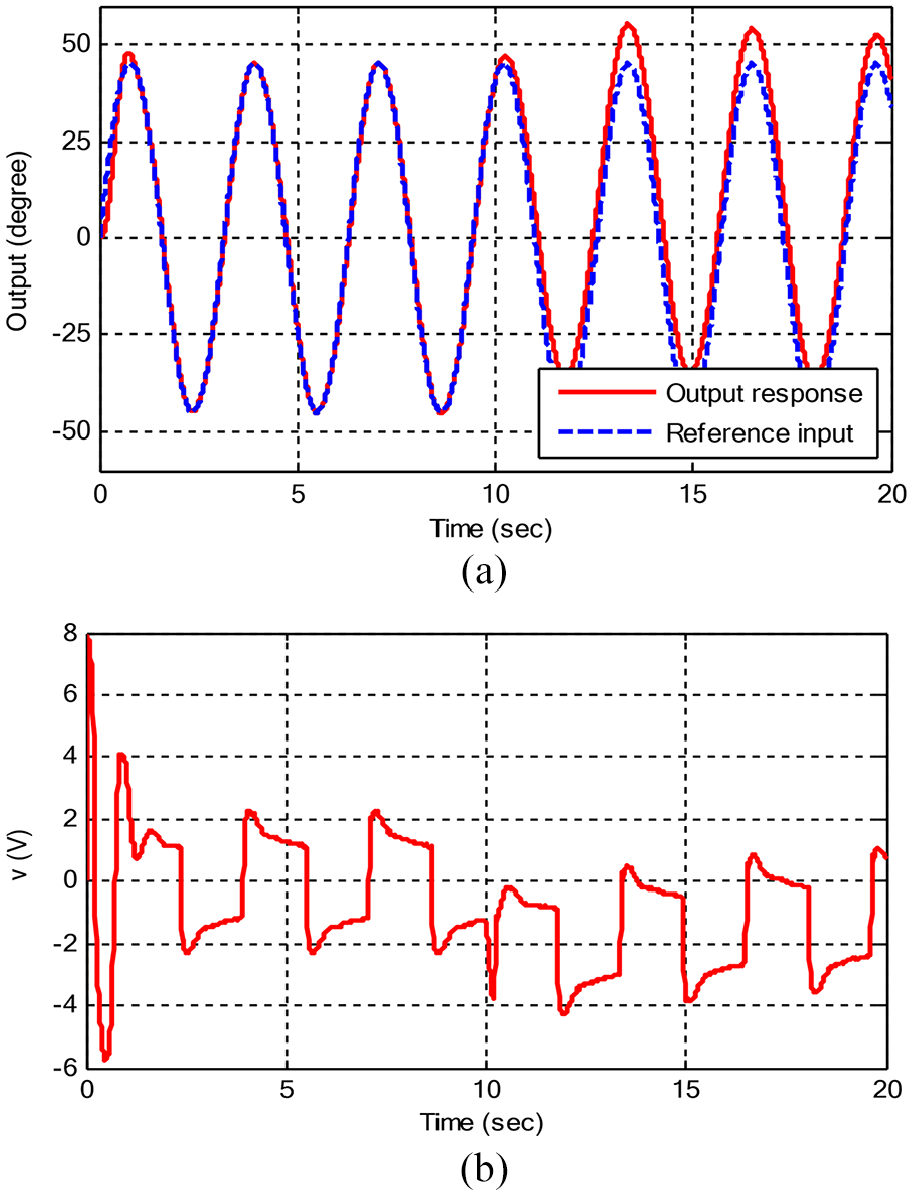
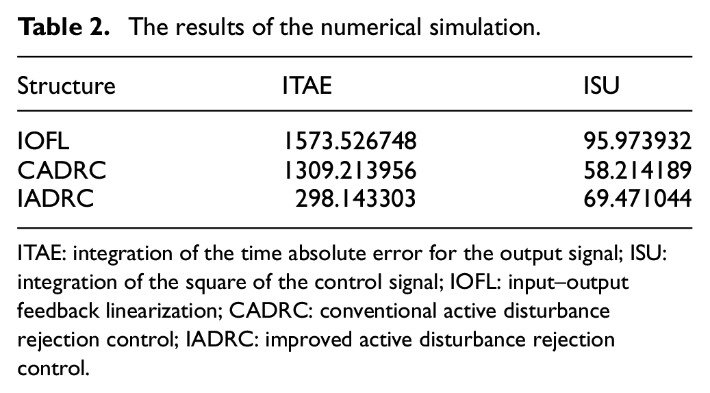
A second simulation scenario is conducted in this work which included the presence of an exogenous disturbance ${\tau }_d$ of type step at t = 10 s with an amplitude of 0.5 Nm and an increase of 40% in the load inertia. The results of the numerical simulation are shown in Figures 6–8. The numerical results of the two performance indices of the second scenario are listed in Table 2. As shown in the table, the ITAE significantly reduced for the IADRC case. This improvement in the transient response, which is reflected by the value of ITAE, occurs with an insignificant increase in the delivered energy to the actuation as compared to CADRC, where both IADRC and CADRC witnessed a big reduction in the control energy as compared to IOFL technique.

Figure 6.

The curves of the numerical simulations for the second scenario using IOFL: (a) the output response of the SLFJM, y and (b) the control signal, v.

Figure 7.

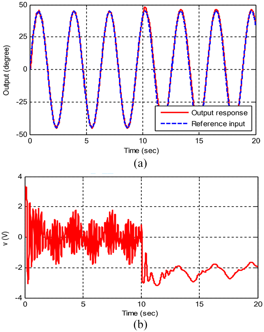
The curves of the numerical simulations for the second scenario using CADRC: (a) the output response of the SLFJM, y and (b) the control signal, v.

Figure 8.

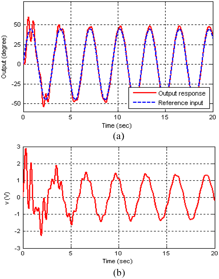
The curves of the numerical simulations for the second scenario using IADRC: (a) the output response of the SLFJM, y and (b) the control signal, v.

Table 2.

The results of the numerical simulation.

Structure	ITAE	ISU
IOFL	1573.526748	95.973932
CADRC	1309.213956	58.214189
IADRC	298.143303	69.471044

ITAE: integration of the time absolute error for the output signal; ISU: integration of the square of the control signal; IOFL: input–output feedback linearization; CADRC: conventional active disturbance rejection control; IADRC: improved active disturbance rejection control.

Adding inertia uncertainty and exogenous disturbance highly affects the performance of the IOFL (see Figure 6) against the other two control schemes as described previously in this paper. The presence of LESO and INLESO in both CADRC and IADRC, respectively, is the reason for the improvement of the reference tracking in these techniques, see Figures 7(a) and 8(a), where both the uncertainty in the inertia and the exogenous disturbance are lumped all together and estimated by the LESO and INLESO and canceled from the input channel of the SLFJM. This process does not exist in traditional IOFL. Moreover, the superiority of the IADRC over the CADRC in terms of reference tracking is the existence of the saturation-like behavior that the error function of the INLESO has, where higher estimated accuracy is obtained with the INLESO than the LESO, and this is reflected in the ITAE values of Table 2 and in the reference tracking of Figures 7(a) and 8(a) beyond 10 s.

Measurement noise scenario

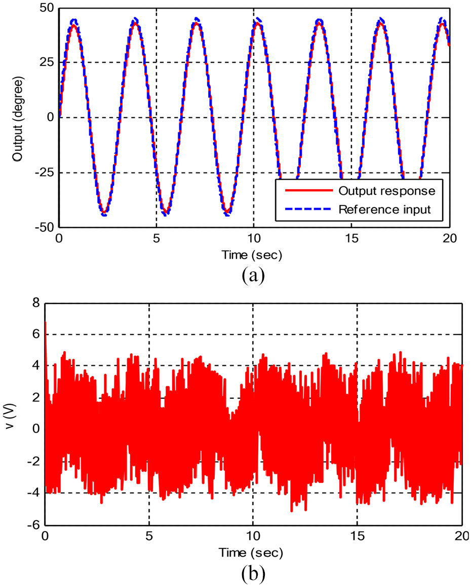
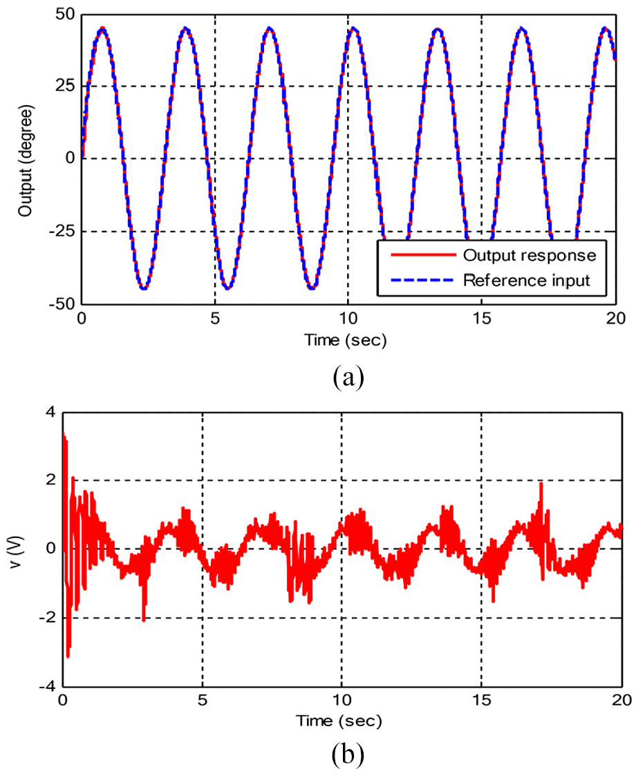
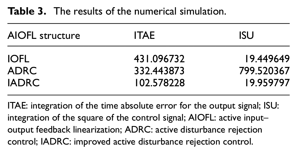
The final scenario that has been demonstrated in this work is testing the immunity of the system against measurement noise. A Gaussian measurement noise at the output is considered; the variance and the mean of the Gaussian noise are 0.0001 and 0, respectively. To actively counteract the effect of the noise, both ESOs are retuned again using GA under the existence of noise based on the OPI defined in equation (90). The newly tuned parameters of the LESO are ${\omega }_0=851.0106$ , ${\alpha }_1=5.40326$ , ${\alpha }_2=0.2871$ , ${\alpha }_3=0.7644$ , ${\alpha }_4=0.01$ , ${\alpha }_5=1.22\times {10}^{-6}$ , and $b_0=33.7432$ . While the new tuned parameters of the INLESO are ${\omega }_0=121.020$ , ${\alpha }_1=0.205$ , ${\alpha }_2=0.6$ , ${\alpha }_3=0.42$ , ${\alpha }_4=0.0232$ , ${\alpha }_5=7.19\times {10}^{-6}$ , and $b_0=9.7$ . The other parameters of both control schemes (CADRC and IADRC) are not changed. The results of the numerical simulation are shown in Figures 9–11. The numerical results of the two performance indices of the second scenario are listed in Table 3. As shown in Table 3, both of the ITAE and ISU are reduced significantly using the IADRC scheme. This improvement in the transient response and the reduced control energy is noticeable in Figure 11.

Figure 9.

The curves of the numerical simulations for the third scenario using IOFL: (a) the output response of the SLFJM, y and (b) the control signal, v.

Figure 10.

The curves of the numerical simulations for the third scenario using CADRC: (a) the output response of the SLFJM, y and (b) the control signal, v.

Figure 11.

The curves of the numerical simulations for the third scenario using IADRC: (a) the output response of the SLFJM, y and (b) the control signal, v.

Table 3.

The results of the numerical simulation.

AIOFL structure	ITAE	ISU
IOFL	431.096732	19.449649
ADRC	332.443873	799.520367
IADRC	102.578228	19.959797

ITAE: integration of the time absolute error for the output signal; ISU: integration of the square of the control signal; AIOFL: active input–output feedback linearization; ADRC: active disturbance rejection control; IADRC: improved active disturbance rejection control.

The presence of measurement noise has approximately no effect on the response of the IOFL due to the nonexistence of any type of observer in this technique as can be seen from Figure 9. In the case of CADRC, the noise is simply bypassed by the LESO which acts a high gain observer with the noise appears on the output channel of LESO where its components are amplified by the gain values of the LESO and consequently deteriorated the control signal v, see Figure 10(b). More specifically, the INLESO of the IADRC attenuates the noise due to its saturation-like behavior with little effect of chattering appears on the control signal v as depicted in Figure 11(b).

Conclusion

This paper addressed the problem of AIOFL for SLFJM, which is a highly nonlinear uncertain system subjected to external disturbances and measurement noise. It differs from the traditional IOFL, which assumes a nominal nonlinear system to work on it. The AIOFL has been implemented by both CADRC and IADRC paradigms, which transforms the nonlinear uncertain system into a chain of integrators. The key point of the proposed method is that it requires only the relative degree of the nonlinear uncertain system. It can be concluded that the proposed IADRC-based AIOFL method transformed the SLFJM uncertain system into a linear one and excellently estimated and canceled the generalized disturbance in a real-time manner. The steady-state observer estimation error is inversely proportional to the bandwidth of the ESO, and the closed-loop system with the proposed AIOFL schemes is globally asymptotically stable based on the Lyapunov stability analysis. While both ADRC-based AIOFL versions presented good tracking, the IADRC-based AIOFL exhibited better performance than CADRC-based AIOFL and traditional IOFL and provided the actuator with a more stable control signal, and it has less fluctuation with small amplitude. Finally, the IADRC-based AIOFL had more immunity to noise than other schemes.