Stochastic time-dependent vehicle routing problem: Mathematical models and ant colony algorithm

Abstract

This article addresses the stochastic time-dependent vehicle routing problem. Two mathematical models named robust optimal schedule time model and minimum expected schedule time model are proposed for stochastic time-dependent vehicle routing problem, which can guarantee delivery within the time windows of customers. The robust optimal schedule time model only requires the variation range of link travel time, which can be conveniently derived from historical traffic data. In addition, the robust optimal schedule time model based on robust optimization method can be converted into a time-dependent vehicle routing problem. Moreover, an ant colony optimization algorithm is designed to solve stochastic time-dependent vehicle routing problem. As the improvements in initial solution and transition probability, ant colony optimization algorithm has a good performance in convergence. Through computational instances and Monte Carlo simulation tests, robust optimal schedule time model is proved to be better than minimum expected schedule time model in computational efficiency and coping with the travel time fluctuations. Therefore, robust optimal schedule time model is applicable in real road network.

Introduction

With the rapid development of e-commerce, the volume of urban delivery rises sharply. In 2013, the total express delivery volume in China reached 9.19 billion parcels, ranked the second in the world, and sustained an annual growth rate of 43.5% over the recent 5 years. ¹ Meanwhile, due to the quick pace of urban life, the requirements for timely delivery also increased continuously. More and more couriers focused on reducing distribution costs and improving customer satisfaction. Some e-commerce companies, such as 360buy.com and Suningshop.com, have built their own distribution systems to cope with the growth of delivery volume and ensure the timeliness of delivery. ²

As a core issue in logistics distribution, vehicle routing problem (VRP) has attracted a lot of research, after it was first proposed by Dantzig and Ramser ³ in 1959. But most research of VRP in the last five decades assumed that the link travel times of networks are static or deterministically time-dependent.

However, due to the increasing heavy urban traffic, traffic congestion has become more frequent, and the urban transportation system has become very vulnerable. Random factors, such as bad weather conditions, incidents, constructions, and special events, can lead to the uncertainty of travel time and cause severe traffic congestion. In order to optimize the delivery performance and improve the customer satisfaction (especially for time-sensitive customers), both the stochastic and time-varying nature of travel time should be considered, not just taking either one into consideration.

The aim of this article is to study the mathematical model and efficient algorithm for the stochastic time-dependent vehicle routing problem (STDVRP). The contributions of this article are as follows:

1. Two mathematical models named robust optimal schedule time (ROST) and minimum expected schedule time (MEST) are proposed for STDVRP, which can ensure delivery within time windows in the stochastic time-dependent (STD) network. ROST model does not require the probability distributions of travel times and can be converted into time-dependent vehicle routing problem (TDVRP).

2. An ant colony optimization (ACO) algorithm is proposed with the improvements of initial solution and transition probability. Both improvements speed up ACO algorithm’s convergence. And ACO algorithm performs well in both TDVRP and STDVRP instances.

3. ROST model performs well in computational efficiency and handling travel time fluctuations. If low fluctuations are considered in ROST model, the solutions can cope with higher fluctuations, with only little increase in delivery cost.

Literature review

STDVRP

STDVRP is extended from TDVRP and stochastic vehicle routing problem (SVRP), which only consider either random or time-dependent property of travel time. In TDVRP, the link travel times are treated as deterministic time-dependent functions. However, they are defined as random variables in SVRP.

TDVRP

Malandraki et al. first proposed a strict mathematical model for TDVRP and formulated the link travel times as piecewise functions of distance and the time of the day. They designed a nearest-neighbor heuristic algorithm and a cut plane heuristic algorithm, and solved TDVRP instances without time windows.^4,5 In order to overcome the defect of waiting at the customer node in Malandraki’s model, Ichoua et al. introduced the First in First out (FIFO) principle into TDVRP and represented the dynamic network by time-dependent function of speed. They put forward a parallel tabu search heuristic and solved TDVRP with time windows. ⁶ Donati et al.^7–9 proposed efficient ant colony algorithms for TDVRP, and applied them in computational instance of real road network.

SVRP

Laporte et al. introduced stochastic travel time into VRP, and proposed three mathematical models: a chance constrained model and two recourse models. They solved SVRP without time windows by a general branch and cut algorithm. ¹⁰ Lambert et al. ¹¹ studied the problem of collection routes for cash and negotiables from bank branches, and designed an improved Clarke & Wright algorithm for SVRP. Kenyon and Morton ¹² put forward two mathematical models for SVRP: one minimized the expected completion time and the other maximized the probability of completion by a pre-specified deadline, and solved them by a branch and cut algorithm.

STDVRP

In contrast to traditional VRP and TDVRP, there have been limited literatures on STDVRP. Lecluyse et al. ¹³ applied queuing theory to analyze the travel time in STDVRP, and used a tabu search algorithm to solve STDVRP without time windows. Nahum et al. developed a chance constrained model for STDVRP without time windows, and designed a saving algorithm and a genetic algorithm (GA). Computational test showed that the results of GA were 3%−5% better than those of saving algorithm. But GA was very time-consuming, for the STDVRP with 100 customers, its computing time was more than 2 h.^14,15 Zhou ¹⁶ studied the financial escorting VRP, developed a minimum expected cost model for STDVRP, evaluated customer satisfaction with maximum delay, and designed a GA algorithm for STDVRP.

STD optimal path problem

For the real road network, there are often many paths between two customers in STDVRP. Therefore, optimal path finding problem is a fundamental sub-problem for VRP. In contrast to STDVRP, there have been much more researches on stochastic time-dependent optimal path problem (STDOPP).

Hall first proposed STDOPP. He chose minimum expected travel time (METT) as the optimal criterion and designed a branch and bound algorithm. He found that, in STD network, the sub-path of shortest path may not be the shortest one, that is, the Bellman’s principle of optimality does not hold. Therefore, the traditional shortest path algorithms cannot be applied directly to STDOPP. ¹⁷ Miller-Hooks and colleagues^18,19 studied STDOPP with the optimal criterion of METT, and proposed two label correcting algorithms with exponential computation complexity. Wellman et al. ²⁰ extended the deterministic consistent condition to STD network and identified a stochastic consistency condition. He presented a revised path planning algorithm based on the optimal criterion of utility. He and Gao ²¹ defined a disutility function of travel time to evaluate the path, and designed a label correcting algorithms satisfying Bellman’s principle.

Most of the above algorithms need a probability distribution of link travel time and had exponential computation complexity. Sim introduced the robust optimization method to optimal path problem in stochastic network, in order to find the minimum travel time path in the worst case. This method only required the variation range of link travel time instead of the probability distribution and had a polynomial computational complexity. ²² Sun et al.^23,24 extended Sim’s method to STDOPP and converted STDOPP into a minimum travel time path problem in time-dependent network, which can be solved by traditional label setting or label correcting algorithms.

Summary of literatures

Most of above research on SVRP and STDVRP used chance constrained model or recourse model. Both models often require probability distributions of travel times. In addition, their computation complexity will be much higher in STDVRP with time windows, because of more chance constrains. Requirement of probability distributions of travel times and high computation complexity are the restraints that most existing approaches of STDOPP cannot be applied into large-scale real network. For the STDVRP in real road network, it is difficult to calibrate the probability distributions of travel times individually. However, robust optimization method provides a new way for STDVRP, as it has better computational tractability and only needs the variation range of travel time.

In this article, we apply robust optimization method to STDVRP so that to ensure that the delivery can meet the requirements of customers’ time window even in the worst case.

Mathematical model for STDVRP

The notations and variables of STDVRP model are listed in Appendix 1.

STD network

Given a directed network $G=(V,A,T,C_{\mathrm{ij}}^t)$ , where V is the set of nodes and A is the set of links. (i, j) represents the directed link from node i to j. T is the set of time intervals {0, 1, …, M − 1}, M is the number of time intervals. $C_{\mathrm{ij}}^t$ denotes the travel time of link (i, j) at time interval t(t ∈ T).

$C_{\mathrm{ij}}^t$ is defined as

$$C_{\mathrm{ij}}^t=R_{\mathrm{ij}}^t+{\delta }_{\mathrm{ij}}^t$$

(1)

$R_{\mathrm{ij}}^t$ is a fixed travel time value at time interval t, and ${\delta }_{\mathrm{ij}}^t$ is a random variable with the range of $[0,d_{\mathrm{ij}}^t]$ , where $d_{\mathrm{ij}}^t$ is also a fixed value at time interval t. Hence, $C_{\mathrm{ij}}^t$ is a random time-dependent variable which takes value within the range of $[R_{\mathrm{ij}}^t,R_{\mathrm{ij}}^t+d_{\mathrm{ij}}^t]$ .

Furthermore, it is assumed that the network satisfies the stochastic consistent condition proposed by Wellman et al. ²⁰ Namely, if for any link (i, j) ∈ A at any time interval t ≤ t′ and any given time ξ, the following inequality holds

$$\mathrm{Pr}(C_{\mathrm{ij}}^t+t\le \xi )\ge \mathrm{Pr}(C_{\mathrm{ij}}^{t\prime }+t\prime \le \xi )$$

(2)

The inequality means that the probability of arriving at time ξ cannot be increased by leaving later. Except for few overtaking in real transportation network, this consistent condition (FIFO property) generally holds.

Robust optimal path in STD network

In this section, robust optimization method with Min-Max Criterion is applied to STDOPP. The optimal criterion is finding the minimum travel time path between two nodes in the worst case, which is defined as robust optimal path.

For any path ${\lambda }_{\mathrm{ij}}^m$ from i to j at time interval m, the travel time in the worst case is

$$\tilde{f}({\lambda }_{\mathrm{ij}}^m)=max\sum _{(a,b)\in {\lambda }_{\mathrm{ij}}^m}\sum _{t=m}^M(R_{\mathrm{ab}}^t+{\tau }_{\mathrm{ab}}^t)·y_{\mathrm{ab}}^t$$

(3)

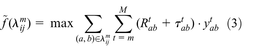
So the travel time of the optimal path $(T_{\mathrm{ij}}^m)$ from i to j at time interval m is

$$T_{\mathrm{ij}}^m=\tilde{f}({\lambda }_{\mathrm{ij}}^{*m})=min(\tilde{f}({\lambda }_{\mathrm{ij}}^m))=min(max\sum _{(a,b)\in {\lambda }_{\mathrm{ij}}^m}\sum _{t=m}^M(R_{\mathrm{ab}}^t+{\tau }_{\mathrm{ab}}^t)·y_{\mathrm{ab}}^t),{\lambda }_{\mathrm{ij}}^m\in {\Lambda }_{\mathrm{ij}}^m$$

(4)

For equation (3), it can be proved that the following equation (5) holds ²³

$$\begin{array}{c}\multicolumn{1}{c}{\tilde{f}({\lambda }_{\mathrm{ij}}^m)=max\sum _{(a,b)\in {\lambda }_{\mathrm{ij}}^m}\sum _{t=m}^M(R_{\mathrm{ab}}^t+{\tau }_{\mathrm{ab}}^t)·y_{\mathrm{ab}}^t}\\ \multicolumn{1}{c}{=\sum _{(a,b)\in {\lambda }_{\mathrm{ij}}^m}\sum _{t=m}^M(R_{\mathrm{ab}}^t+d_{\mathrm{ab}}^t)·y_{\mathrm{ab}}^t}\end{array}$$

(5)

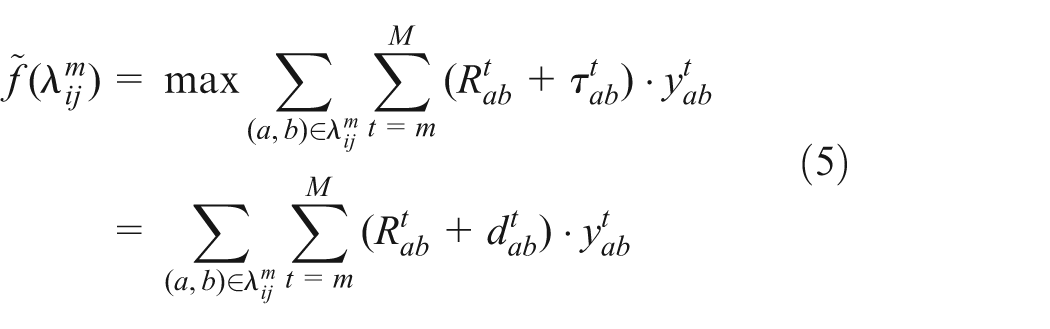
Therefore, the travel time of the optimal path from i to j at time interval m is

$$\begin{array}{c}\multicolumn{1}{c}{T_{\mathrm{ij}}^m=min(\tilde{f}({\lambda }_{\mathrm{ij}}^m))}\\ \multicolumn{1}{c}{=min(\sum _{(a,b)\in {\lambda }_{\mathrm{ij}}^m}\sum _{t=m}^M(R_{\mathrm{ab}}^t+d_{\mathrm{ab}}^t)·y_{\mathrm{ab}}^t),{\lambda }_{\mathrm{ij}}^m\in {\Lambda }_{\mathrm{ij}}^m}\end{array}$$

(6)

In equation (6), $R_{\mathrm{ab}}^t+d_{\mathrm{ab}}^t$ is the upper bound of travel time of link (a, b) at time interval m, which changes along with the time interval. For any link (a, b) in network G, if let $R_{\mathrm{ab}}^t+d_{\mathrm{ab}}^t$ as the travel time of link (a, b), we get a new time-dependent network G′. It can be proved that G′ satisfies FIFO property. ²³ Thus, the STDOPP can be converted into a minimum travel time path finding problem in a time-dependent network G′ with FIFO property. Therefore, the traditional label setting or label correcting algorithms can be applied to solve this problem with polynomial computational complexity.

ROST model

In this article, we study STDVRP with hard time windows. It is assumed that there is only one depot where the delivery routes start and end, vehicles have same capacity, the demands of customers are pre-determined, and each customer must be served within his/her time window. If the vehicle arrives early at the customer node, it should wait to serve till the beginning of the time window. As STDVRP is a multi-objective optimization problem, in this article, we mainly consider the number of utilized vehicles and total schedule time. Moreover, the former is considered to be more important than the latter.

The following is the ROST model for STDVRP, which minimizes the number of utilized vehicles and the total schedule time in the worst case.

Objective function

$$minz={\alpha }_1\times K+{\alpha }_2\times \mathrm{ST}$$

(7)

Expressions of objective function

$$\mathrm{ST}=\mathrm{TT}+\mathrm{WT}+\mathrm{SVT}$$

(8)

$$\mathrm{TT}=\sum _{i\in \mathrm{SD}}\sum _{\genfrac{}{}{0ex}{}{j\in \mathrm{DE}}{j\ne i}}\sum _{m=1}^M(T_{\mathrm{ij}}^m·x_{\mathrm{ij}}^m)$$

(9)

$$\mathrm{WT}=\sum _{i\in D}max(e_i-t_i,0)$$

(10)

$$T_{\mathrm{ij}}^m=min(\sum _{(a,b)\in {\lambda }_{\mathrm{ij}}^m}\sum _{t=m}^M(R_{\mathrm{ab}}^t+d_{\mathrm{ab}}^t)·y_{\mathrm{ab}}^t),{\lambda }_{\mathrm{ij}}^m\in {\Lambda }_{\mathrm{ij}}^m$$

(11)

$$\mathrm{SVT}=\sum _{i\in D}\mathrm{sv}{t}_i$$

(12)

Subject to

$$\sum _{\genfrac{}{}{0ex}{}{i\in \mathrm{SD}}{j\ne i}}\sum _{m=1}^M{x}_{\mathrm{ij}}^m=1,j\in \mathrm{DE}$$

(13)

$$\sum _{\genfrac{}{}{0ex}{}{j\in \mathrm{DE}}{i\ne j}}\sum _{m=1}^M{x}_{\mathrm{ij}}^m=1,i\in \mathrm{SD}$$

(14)

$$\begin{array}{c}\multicolumn{1}{c}{\sum _{k=1}^{K}k(v_{\mathrm{ik}}-v_{\mathrm{jk}})\le B(1-\sum _{m=1}^M{x}_{\mathrm{ij}}^m),i\in \mathrm{SD},j\in \mathrm{DE},i\ne j}\end{array}$$

(15)

$$\sum _{k=1}^{K}k(v_{\mathrm{ik}}-v_{\mathrm{jk}})\ge B(\sum _{m=1}^M{x}_{\mathrm{ij}}^m-1),i\in \mathrm{SD},j\in \mathrm{DE},i\ne j$$

(16)

$$\sum _{k=1}^K{v}_{\mathrm{ik}}=1,i\in D$$

(17)

$$\sum _{i\in D}(q_i·v_{\mathrm{ik}})\le Q_k,k=1,2,3,4$$

(18)

$$\sum _{i\in S}\sum _{j\in \mathrm{DE}}\sum _{m=1}^M{x}_{\mathrm{ij}}^m=\sum _{i\in \mathrm{SD}}\sum _{j\in E}\sum _{m=1}^M{x}_{\mathrm{ij}}^m$$

(19)

$$\sum _{\genfrac{}{}{0ex}{}{i,j\in \mathrm{SC}}{i\ne j}}\sum _{m=1}^M{x}_{\mathrm{ij}}^m\le \left|\mathrm{SC}\right|-1,\mathrm{SC}\in D$$

(20)

$$t_j=max(e_i,t_i)+\mathrm{sv}{t}_i+T_{\mathrm{ij}}^m\le l_j,j\in D$$

(21)

$$t_{\mathrm{depot}}^k\le l_0$$

(22)

Objective function (7) minimizes the number of utilized vehicles and the total schedule time, where α ₁ and α ₂ are weighted coefficients. As the number of utilized vehicles is more important, α ₁ should be assigned to a larger value. Total schedule time (ST) is the sum of total travel time (TT), waiting time (WT), and total service time (SVT). The optimal path between two nodes is defined as the robust optimal path in equation (11).

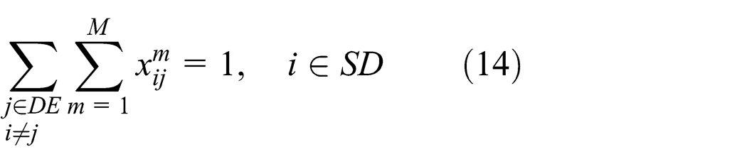
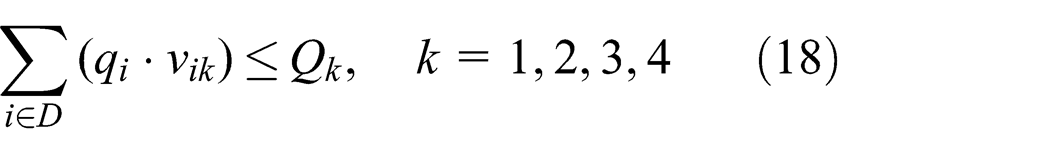
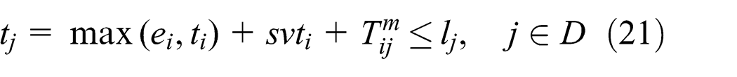
Constraints (13 and 14) state that each customer can be served only once. Constraints (17–19) state that the customers in each route can only be served by one vehicle. Constraint (18) states that the demands of customers in each route cannot exceed the capacity of the vehicle. Constraint (19) states that all the utilized vehicles should return to the depot. Constraint (20) is added for route continuity. Constraints (21 and 22) ensure the satisfaction of time windows.

In the ROST model, the optimal path is computed based on the upper value of link travel time. Therefore, ROST model is equivalent to a TDVRP model in network G′.

MEST model

If the optimal path is defined as the path of METT, we can formulate the MEST model for STDVRP.

In MEST model, the travel time of optimal path $(T_{\mathrm{ij}}^m)$ is defined as

$$T_{\mathrm{ij}}^m=\overline{f}({\lambda }_{\mathrm{ij}}^{*m})=min(\overline{f}({\lambda }_{\mathrm{ij}}^m)),{\lambda }_{\mathrm{ij}}^m\in {\Lambda }_{\mathrm{ij}}^m$$

(23)

${\lambda }_{\mathrm{ij}}^{*m}$ denotes the path of METT from i to j at time interval m, and the worst-case travel time of ${\lambda }_{\mathrm{ij}}^{*m}$ is $\tilde{f}({\lambda }_{\mathrm{ij}}^{*m})$ which can be calculated by equation (5).

Let ${\tilde{t}}_i$ and ${\tilde{t}}_j$ be the latest arrive time at customer node i and j, and let ${\tilde{t}}_{\mathrm{depot}}^k$ be the latest return time of vehicle k to depot.

In order to satisfy the requirement of time windows, defined constraints as

$${\tilde{t}}_j=max(e_i,{\tilde{t}}_i)+\mathrm{sv}{t}_i+\tilde{f}({\lambda }_{\mathrm{ij}}^{*m})\le l_j,j\in D$$

(24)

$${\tilde{t}}_{\mathrm{depot}}^k\le l_0$$

(25)

The other parts of objective function and constraints in MEST model are the same as those in ROST model.

The MEST model is similar to chance constrained model. The chance constrained model ensures that the probability of completing delivery within time windows is larger than a pre-specified value. However, in the MEST model, completing delivery within time windows is 100% guaranteed.

The expected travel time of path should be computed in MEST model, which needs the probability distributions of travel times. Through statistical analysis, Zhou ¹⁶ found the expected travel time can be calculated approximately by the expected link speed. Therefore, in the ACO algorithm for MEST model, Zhou’s method is applied to calculate the expected travel time.

ACO algorithm

ACO algorithm is proposed by Dorigo et al., ²⁵ which builds solutions by simulating the communication and collaboration of ants. Donati et al. ⁷ designed an ACO algorithm for TDVRP. Local search procedures were added in such algorithm to accelerate the speed of convergence. Furthermore, Donati et al. ⁹ put forward a multi-ant colony system, which solves the bi-objective optimization problem (minimize both the number of utilized vehicles and total travel time) by the cooperation of two ant colonies.

In this article, in order to speed up the convergence, we designed an ACO algorithm with the following improvement:

1. Generate the initial solution by an efficient route construction algorithm named nearest-neighbor algorithm based on minimum cost (NNC). ²⁶

2. Design a new customer node choice method by the transition probability considering both travel time and time windows.

Procedures of ACO algorithm

The procedures of ACO algorithm for STDVRP are as follows:

Step 1: initialization

Generate the initial solution by NNC algorithm, and set the initial pheromone value of each link. Then, update the pheromone of each link by the rule of Ant-cycle model.

• (a) Initial solution

NNC is an efficient route construction algorithm for TDVRP, ²⁶ which is extended from Solomon’s ²⁷ nearest-neighbor (NN) algorithm for VRP.

Here, we apply NNC algorithm to generate the initial solution for ACO algorithm.

• (b) Initial pheromone

The initial pheromone τ ₀ of each link is determined by

$${\tau }_0=\frac{1}{n·\mathrm{ST}(0)}$$

(26)

In equation (26), n is the number of customer nodes, ST(0) is the total schedule time of the initial solution.

• (c) Ant-cycle model

In Ant-cycle model, ²⁸ the pheromone increment $\Delta {\tau }_{\mathrm{ab}}$ of link (a, b) is defined as

$$\Delta {\tau }_{\mathrm{ab}}=\{\begin{array}{c}\hfill \frac{Q}{\mathrm{ST}(0)},\mathrm{if}\mathrm{link}(a,b)\in {\lambda }_{\mathrm{ij}}^{*m}\hfill \\ \multicolumn{1}{c}{0,\mathrm{otherwise}}\end{array}$$

(27)

In equation (27), ${\lambda }_{\mathrm{ij}}^{*m}$ is the optimal path from node i to j at time interval m. In the ROST model, ${\lambda }_{\mathrm{ij}}^{*m}$ is the robust optimal path; however, in the MEST model, it is the path with METT. Q is a constant parameter which is set as the value of 10.

Step 2: construct route by ant moving, and update pheromone locally

Each ant departures from the depot, and chooses the next customer node by transition probability and pseudo-random-proportional rule. If the capacity and time window constraints are satisfied, then the customer node will be visited and recorded in the tabu table, otherwise, the ant will return to the depot and construct a new route. Repeat the route construction procedure, until all customer nodes have been visited, thus the ant complete a tour.

• (a) Transition probability

The transition probability is defined as

$$p_{\mathrm{ij}}^s=\{\begin{array}{c}\hfill \frac{{\tau }_{\mathrm{ij}}^{\alpha }(u)·{\eta }_{\mathrm{ij}}^{\beta }(u)}{\sum _{k\in \mathrm{allowed}{}_s}{\tau }_{\mathrm{ik}}^{\alpha }(u)·{\eta }_{\mathrm{ik}}^{\beta }(u)},j\in \mathrm{allowe}{d}_s\hfill \\ \multicolumn{1}{c}{0,j\notin \mathrm{allowe}{d}_s}\end{array}$$

(28)

In equation (28), $p_{\mathrm{ij}}^s$ is the probability of moving from node i to j for ant s. τ_ij (u) is the pheromone value of the optimal path ${\lambda }_{\mathrm{ij}}^{*m}$ in iteration u. η_ij (u) is the visibility of ${\lambda }_{\mathrm{ij}}^{*m}$ determined by equation (29) or (30). α and β are positive parameters. allowed_s is the set of unvisited customer nodes of ant s.

Lu ²⁹ defined η_ij (u) as

$${\eta }_{\mathrm{ij}}(u)=\frac{1}{T_{\mathrm{ij}}(u)}$$

(29)

In equation (29), T_ij (u) is the travel time of ${\lambda }_{\mathrm{ij}}^{*m}$ in iteration u.

Here, we give a new method considering both travel time and time windows to define η_ij (u) as

$${\eta }_{\mathrm{ij}}(u)=\frac{1}{({\gamma }_1·T_{\mathrm{ij}}(u)+{\gamma }_2·W_{\mathrm{ij}}+{\gamma }_3·E_{\mathrm{ij}})}$$

(30)

In equation (30), W_ij denotes the nearness of time windows between node i and j, which is determined by

$$W_{\mathrm{ij}}=max(e_j,t_j)-(max(e_i,t_i)+\mathrm{sv}{t}_i)$$

(31)

E_ij denotes the urgency of node j, which is defined as

$$E_{\mathrm{ij}}=l_j-(max(e_i,t_i)+\mathrm{sv}{t}_i+T_{\mathrm{ij}}(u))$$

(32)

In equation (32), γ ₁, γ ₂, and γ ₃ are positive coefficients, which satisfy ${\gamma }_1+{\gamma }_2+{\gamma }_3=1$ and are assigned by random values.

• (b) Pseudo-random-proportional rule

The procedure of pseudo-random-proportional rule proposed by Dorigo and Gambardella ³⁰ is: sample a random number $0\le \epsilon \le 1$ ; if $\epsilon \le {\epsilon }_0$ (ε ₀ is a pre-determined parameter), then ant s move to the node which has the maximum value of $[{\tau }_{\mathrm{ij}}(u){]}^{\alpha }·[{\eta }_{\mathrm{ij}}(u){]}^{\beta }$ ; otherwise, ant s chooses the next node by $p_{\mathrm{ij}}^s$ .

• (c) Update pheromone locally

After an ant moves from one node to another, it should update the pheromone value of the passed links. The pheromone update process in link $(a,b)\in {\lambda }_{\mathrm{ij}}^{*m}$ is defined as

$$\tau {}_{\mathrm{ab}}(u+1)=(1-\rho ){\tau }_{\mathrm{ab}}(u)+\rho {\tau }_0$$

(33)

In equation (33), τ ₀ is determined by equation (26); ρ is a pre-determined parameter called evaporation coefficient, which satisfies $0<\rho <1$ .

Step 3: local search procedure

Local search procedures are very useful for improving the quality of solution.^7,31 After each ant has completed its delivery tour, we apply local search procedures to the routes to get better solutions, which include two-opt exchange, or-opt exchange, node relocation and λ-interchange. ³¹

• (a) Two-opt exchange: two edges in the route are replaced by another two edges;

• (b) Or-opt exchange: move a sub-path in the route to a new location;

• (c) Node relocation: move a node to a new location in the route;

• (d) λ-interchange: select a sub-path from two routes respectively, and exchange them. The length of each sub-path should less than λ.

Step 4: update pheromone globally

After all ants have finished their tours, update the pheromone value of the links in the best solution, which has the least utilized vehicles and the least total schedule time till iteration u. Let BL be the set of links in the route of the best solution. The pheromone update process is defined as

$$\tau {}_{\mathrm{ab}}(u+1)=(1-\rho ){\tau }_{\mathrm{ab}}(u)+\rho \Delta {\tau }_{\mathrm{ab}}(u,u+1)$$

(34)

$$\Delta {\tau }_{\mathrm{ab}}(u,u+1)=\{\begin{array}{c}\hfill \frac{1}{\mathrm{ST}(u)},\mathrm{if}\mathrm{Link}(a,b)\in \mathrm{BL}\hfill \\ \multicolumn{1}{c}{0,\mathrm{otherwise}}\end{array}$$

(35)

In equation (35), ST(u) is the total schedule time of the best solution till iteration u.

Step 5: check the termination condition

If it has reached the pre-determined maximum number of iterations, go to step 6; otherwise, return to step 2.

Step 6: output the best solution and stop the algorithm

Pheromone update rule of Max-Min ant system

In order to avoid prematurity or early search stagnation problem, a pheromone update rule named Max-Min ant system is applied in the ACO algorithm, ³² which restricts the pheromone value of each link in the range of [τ _min, τ _max]. The upper bound τ _max is determined by

$${\tau }_{max}=\frac{1}{\mathrm{ST}(u)}$$

(36)

τ _min is determined by

$${\tau }_{min}=\frac{{\tau }_{max}(1-\sqrt[n]{\omega })}{(n/2-1)\sqrt[n]{\omega }}$$

(37)

In equation (37), n is the number of customer nodes, ω is the constant parameter which is set as the value of 0.05.

Computational instances and analysis

In this section, computational instances of STDVRP and TDVRP are constructed, and the Monte Carlo simulation method is introduced to test the solutions in STD network. Then, the performance of ACO algorithm is analyzed in TDVRP instances. In order to analyze the effect of fluctuation of traffic status, the delivery-route plans of solutions for TDVRP instances are tested in STD network. At last, STDVRP instances are solved by both ROST and MEST models. The solutions of the two models are compared and analyzed. Moreover, for ROST model, the ability of coping with higher fluctuations is tested.

Computational instances

In this article, we extend Solomon Instances to STDVRP, which are classical benchmark problems for traditional VRP. Solomon Instances include six sets of problems, ³³ and the number of customers in each problem is 100. Table 1 shows the number of problems, capacity of each vehicle, closing time of depot, service time of each customer, spatial distribution of customers and width of time windows in each set of problems.

Table 1.

Solomon Instances. ³³

Set	Number of problems	Capacity of vehicle	Closing time of depot	Service time of customer	Spatial distribution of customers	Width of time windows
C1	9	200	1236	90	Clustered	Small
C2	8	700	3390	90	Clustered	Large
R1	12	200	230	10	Random	Small
R2	11	1000	1000	10	Random	Large
RC1	8	200	240	10	Mixed	Small
RC2	8	1000	960	10	Mixed	Large

We add time-dependent function of travel speed and the fluctuation of travel speed to Solomon Instances, and get the computational instances for STDVRP.

In the network, four types of links are defined. The time-dependent functions of travel speed are defined in Table 2, with four equal time intervals to represent the peak-hour and off-peak period in real transportation networks.

Table 2.

Time-dependent functions of travel speed.

Link type	v 1	v 2	v 3	v 4
1	1.60	2.00	1.60	2.00
2	1.40	1.80	1.40	1.80
3	1.30	1.50	1.30	1.50
4	1.20	1.40	1.20	1.40

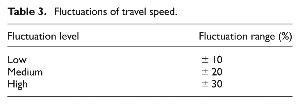
In order to describe the random fluctuation of traffic status, three levels of fluctuation of travel speed are defined in Table 3, for each link in every interval.

Table 3.

Fluctuations of travel speed.

Fluctuation level	Fluctuation range (%)
Low	±10
Medium	±20
High	±30

Let link (i, j) be the path between customer node i and j. The type of link (i, j) is determined by equation (38), where $\mathrm{Mod}((i+j),4)$ is the remainder of (i + j) divided by 4

$$\mathrm{Type}(i,j)=\mathrm{Mod}((i+j),4)+1$$

(38)

In this way, we get 6 sets of 56 problems for STDVRP. Moreover, if the fluctuation of travel speed is set to be 0, 6 sets of 56 counterpart problems are obtained for TDVRP.

Test method and environment

Monte Carlo simulation is applied to generate the link travel speed following uniform distribution, within the range defined in Tables 2 and 3. In this way, the delivery-route plans of solutions for STDVRP instances can be tested. In order to analyze the effect of fluctuation, we also test the solutions for the counterpart instances of TDVRP.

Testing each solution 100 times, we can get the expected values of schedule time, travel time, waiting time, and number of delay in STD network. Number of delay represents how many customer nodes fail to be served before the upper bounds of their time windows due to the travel time fluctuations.

The computation and test environment in this article is as follows:

• CPU: Intel Core i7-3537U (4 cores), 2.00GHz;

• RAM: 8 GB;

• Operation system: Windows 8 (64 bit);

• Programming language: Microsoft C#.

Performance analysis of ACO algorithm

Analysis of convergence

We analyzed the convergence of ACO algorithm by the RC101 problem in Solomon Instances of TDVRP.

The values of parameters in ACO algorithm are as follows: α = 2, β = 10, ρ = 0.4, ε ₀ = 0.3, number of ants is set to be 10 and number of iteration is set as 200.

For Solomon Instances, the values of coefficients in objective function (7) are α ₁ = 10,000 and α ₂ = 1.

In order to analyze the effect of the improvements in initial solution and transition probability, the following three versions of ACO algorithm are tested:

1. ACO1: generate the initial solution randomly and define the transition probability as equation (29);

2. ACO2: generate the initial solution randomly and define the transition probability as equation (30);

3. ACO3: generate the initial solution by NNC algorithm and define the transition probability as equation (30).

The values of initial solutions for RC101 are as follows:

• Initial solution generated randomly: number of utilized vehicles is 63, schedule time is 9488.29;

• Initial solution generated by NNC algorithm: number of utilized vehicles is 14, schedule time is 2643.56.

The computational results of three ACO versions for RC101 are shown in Table 4. The solution quality of ACO3 is slightly better than ACO2, and far outweighs ACO1.

Table 4.

Computational results of three ACO versions for RC101.

Version	Number of vehicles	Schedule time	Travel time	Distance	Waiting time	CPU time (s)
ACO1	18	3183.81	1551.53	2331.93	632.28	12.6
ACO2	13	2503.85	1241.77	1857.08	262.08	45.1
ACO3	13	2472.62	1178.16	1789.73	294.46	45.7

ACO: ant colony optimization algorithm.

The convergence processes of three ACO versions are illustrated in Figure 1. As considering both travel time and time windows in node choice, the convergence speed of ACO2 is much faster than ACO1. Due to a better initial solution, the solution of ACO3 at about the 70th iteration is close to the best solution of ACO2, and the solution is further improved after the 70th iteration.

Figure 1.

Comparison of convergence for three ACO versions.

The computing time of ACO3 and ACO2 is about 45 s, which is 3 times longer than ACO1, due to the increase in computation complexity in transition probability.

Through above analysis, it is noted that the new approaches in initial solution and transition probability can improve the performance of ACO algorithm.

Solomon Instances of TDVRP

We solved Solomon Instances of TDVRP with NNC algorithm and ACO algorithm, respectively, and obtained the average results of different problem sets and all instances in Tables 5 and 6.

Table 5.

Computational results of NNC for TDVRP instances.

Set	Number of vehicles	Schedule time	Travel time	Waiting time	CPU time (ms)
C1 a	10.33	10480.79	977.69	503.10	12.13
C2	3.38	10349.95	750.86	599.09	25.41
R1	11.92	2365.09	1037.42	327.67	10.40
R2	3.00	2600.95	1082.96	517.99	28.44
RC1	12.00	2436.59	1160.33	276.26	15.61
RC2	3.38	2727.28	1283.42	443.86	23.44
Average b	7.48	4918.38	1048.53	441.28	18.97

NNC: nearest-neighbor algorithm based on minimum cost; TDVRP: time-dependent vehicle routing problem.

a

C1: the average test result of problems in set C1 (nine problems).

b

Average: the average test result of all problems (56 problems).

Table 6.

Computational results of ACO for TDVRP instances.

Set	Number of vehicles	Schedule time	Travel time	Waiting time	CPU time (s)
C1	10.00	9903.22	829.59	73.63	61.83
C2	3.38	9680.28	654.03	26.26	122.65
R1	11.25	2131.47	984.56	146.92	59.54
R2	3.00	2065.90	998.77	67.13	118.16
RC1	11.25	2207.23	1080.06	127.17	56.53
RC2	3.38	2340.40	1257.04	83.35	112.74
Average	7.18	4486.69	967.80	90.33	87.61

ACO: ant colony optimization algorithm; TDVRP: time-dependent vehicle routing problem.

Compared with NNC algorithm, the number of utilized vehicles, schedule time, and waiting time of the solutions of ACO algorithm are reduced by 4.01%, 8.78%, and 79.53%, respectively. As there is no TDVRP benchmark, we cannot evaluate the solution quality of ACO directly, but we can refer to the good performance of NN algorithm (VRP version of NNC) in traditional VRP. For the Solomon Instances of traditional VRP, the solutions of NN algorithm are close to the known best solutions. ²⁷

Moreover, ACO algorithm performs well in computational efficiency, where the average computing time of all Solomon Instances is 87.61 s.

Test solutions of TDVRP in STD networks

Using Monte Carlo simulation, we tested the delivery-route plans of solutions for TDVRP instances in the STD networks with travel speed at three fluctuation levels.

Table 7 shows the average results of the solutions generated by ACO and NNC algorithm for all TDVRP instances (for details see Tables 10 and 11 in Appendix 2).

Table 7.

Average test results of TDVRP instances’ solution in STD networks.

Algorithm	Fluctuation level	Expected schedule time	Expected travel time	Expected waiting time	Expected number of delay
ACO	Low	4489.11	970.92	89.62	0.49
	Medium	4496.64	979.93	88.15	1.24
	High	4510.42	996.20	85.65	2.35
NNC	Low	4920.67	1051.91	440.19	0.94
	Medium	4927.87	1061.78	437.52	2.31
	High	4941.18	1079.77	432.84	4.29

TDVRP: time-dependent vehicle routing problem; STD: stochastic time-dependent; ACO: ant colony optimization algorithm, NNC: nearest-neighbor algorithm based on minimum cost.

Effect of travel time fluctuations on the solutions of ACO algorithm for TDVRP

For the test results of ACO algorithm, compared with the values of TDVRP solution in Table 6, the expected schedule time and expected travel time increase slightly (<3%), but the expected waiting time decrease a little (<6%).

With the rising of travel time fluctuations, the number of delay increases gradually and reaches 2.35 at high fluctuation level. Therefore, the effect of fluctuations on TDVRP solutions of ACO algorithm is not significant, for the waiting times (averages 90.33) of TDVRP solutions (Table 6) provides a certain redundancy to fluctuations.

Comparison of ACO and NNC algorithm

The effect of travel time fluctuations on the solutions of NNC algorithm is more significant than ACO algorithm. Compared with NNC algorithm, at high fluctuation level, the expected number of delay of ACO algorithm reduces by 45.22%, but the expected schedule time, expected travel time, and expected waiting time also reduce by 8.72%, 7.74%, and 80.21%, respectively. It means that the delivery-route plans of ACO algorithm are tighter but cope with fluctuations better than those of NNC algorithm.

Effect of travel time fluctuations on the solution of different problem sets

Figure 2 illustrates the expected number of delay of ACO algorithm’s solutions for different sets of TDVRP problems in the simulation test.

Figure 2.

Expected number of delay of ACO’s solutions for TDVRP in STD networks.

In STD networks at different fluctuation levels, the number of delay in Type-1 problems (C1, R1, and RC1) is larger than that in Type-2 problems (C2, R2, and RC2). The reason is the time windows of Type-2 problems are larger than Type-1 problems, which leaves more room to cope with the travel time fluctuations.

In addition, the number of delay in C problems is less than that in R and RC problems, which is because the customer nodes in C problems are more clustered, making the variation of travel time between nodes smaller.

Computation and test for STDVRP instances

We applied both ROST model and MEST model to Solomon Instances of STDVRP in the STD networks with travel speed at three fluctuations levels, and obtained six groups of STDVRP instances (two types of models, and three types of STD networks with different fluctuation), where each group has 56 problems.

Then, we solved them by ACO algorithm, and the average solution values (number of utilized vehicles and computing time) of each group of STDVRP instances are shown in Table 8.

Table 8.

Computation and test results of STDVRP instances.

Model	Fluctuation level	Number of vehicles	CPU time (s)	Expected schedule time	Expected travel time	Expected waiting time	Expected number of delay
ROST	Low	7.36	89.37	4545.00	968.73	147.70	0
	Medium	7.59	86.95	4573.05	949.52	194.96	0
	High	7.86	85.22	4695.62	957.10	309.95	0
MEST	Low	7.30	116.14	4526.65	984.57	113.51	0
	Medium	7.63	113.39	4604.04	1014.27	161.19	0
	High	7.95	110.36	4691.03	1041.81	220.65	0

STDVRP: stochastic time-dependent vehicle routing problem; ROST: robust optimal schedule time model; MEST: minimum expected schedule time model.

Furthermore, by Monte Carlo simulation, we tested the delivery-route plans of STDVRP solutions in the corresponding STD network, and the average results (expected schedule time, expected travel time, expected number of delay) of each group instances are listed in Table 8 (for details see Tables 12 and 13 in Appendix 2).

Comparison of ROST model and MEST model

As shown in Table 8, the number of utilized vehicles and the expected schedule time of the solutions for ROST model are very close to those of MEST model. At low fluctuation level, the number of utilized vehicles of ROST model is 0.82% larger than that of MEST model. But at medium and higher fluctuation levels, the former is 0.52% and 1.13% less than the latter.

In the Monte Carlo simulation, the expected travel time of ROST model is 1.61%, 6.38%, and 8.13% less than that of MEST model at low, medium, and high fluctuation levels, respectively. So, if only the travel time is considered, the delivery-route of ROST model is better than that of MEST model. The expected waiting time of ROST model is 30.12%, 20.95%, and 40.47% larger than that of MEST model in STD networks at low, medium, and high fluctuation levels, respectively. This means the solutions of ROST model have more redundancy to fluctuations of traffic status than those of MEST model.

The computing time of ACO algorithm in ROST model is 80–90 s. It is about 20% less than that in MEST model, because MEST model performs additional computation of worst-case travel time for time windows constraints. Therefore, the computational performance of ROST model is acceptable.

The number of delay is 0 in ROST and MEST models, because both of them can guarantee delivery within time windows even in the worst case.

Comparison of ROST model and TDVRP model

According to Tables 6–8, compared with the counterpart solutions (ACO algorithm) for TDVRP model, in the solutions for ROST model, the number of utilized vehicles increases by 2.51%, 5.71%, and 9.47%, expected schedule time increases by 1.25%, 1.70%, and 4.11%, and expected waiting time increases by 64.81%, 121.17%, and 261.88%. But there is no delay in the solutions for ROST model.

That is, 2%−10% more vehicles are dispatched in ROST model to guarantee delivery within time windows.

With regard to the computational performance of ACO algorithm, ROST model is very close to TDVRP model.

Redundancy of ROST model’s solutions

For convenience purpose, we define the solutions of ROST model in the STD network with low travel speed fluctuations as Solutions-Low. Then, the delivery-route plans of Solutions-Low in the STD network are tested with medium and high fluctuations, and the average results are shown in Table 9 (for details see Table 14 in Appendix 2).

Table 9.

Average test results of Solutions-Low in STD networks with higher fluctuations.

Fluctuation level	Expected schedule time	Expected travel time	Expected waiting time	Expected number of delay
Medium	4549.18	978.22	142.39	0.06
High	4557.04	994.06	134.40	0.37

STD: stochastic time-dependent.

According to Table 9, compared with the counterparts of solutions (ACO algorithm) for TDVRP model, the number of delay of Solutions-Low reduces by 95.16% and 84.26% at medium and high fluctuation levels, respectively. But the number of utilized vehicle of Solutions-Low is only 2.51% larger than that of TDVRP solutions.

This means, Solutions-Low outperforms TDVRP solutions, as it improves the ability of delivery-route plans to cope with higher fluctuations with only little increase in delivery cost.

Conclusion and future research

Through above computation and test analysis, we can draw the following conclusions:

1. The proposed ACO algorithm performs well in both TDVRP and STDVRP instances. Compared with NNC algorithm, the solutions of ACO algorithm for TDVRP cope with travel time fluctuations better in STD network.

2. For TDVRP instances, if the time windows are tight and spatial distributions of customer nodes are dispersive, the solutions will be susceptible to the travel time fluctuations.

3. For STDVRP instances, solutions of ROST model are equivalent to those of MEST model in delivery cost, but have a better redundancy to fluctuations. The computational efficiency of ROST model is also better than MEST model. Moreover, ROST model only needs the variation range instead of the probability distributions of travel times, which can be derived from historical traffic data.

4. Compared with TDVRP model, ROST model needs 2%−10% more vehicles, but can guarantee delivery within time windows. Furthermore, if low fluctuations are considered in ROST model, the solutions can cope with higher fluctuations, with only little increase in delivery cost, compared with the solutions of TDVRP model.

The delivery cost in ROST model is slightly higher, but it avoids the loss of additional delivery due to failure of delivery within time windows of customers. For real logistics distribution, the carriers should balance the issues of timeliness and cost. For the time-sensitive customers, ROST model can be applied to ensure their time windows are met properly. For other customers, low fluctuations can be considered in ROST model with only a little additional cost, but most customers’ expected time windows are guaranteed.

We have assumed uniform distributed link travel speeds in the Monte Carlo simulation, which may differ from the real traffic status. Therefore, an improved simulation of link travel speed could be adopted in further research. In addition, utility theory can be applied to evaluate the customer satisfactory based on delivery delay.