Sage Journals: Discover world-class research

Abstract

The mode of automotive maintenance chain is gaining more and more attention in China because of its advantages such as the lower cost, higher speed, higher availability, and strong adaptability. Since the automobile chain maintenance parts delivery problem is a very complex multi-depot vehicle routing problem with time windows, a virtual center depot is assumed and adopted to transfer multi-depot vehicle routing problem with time windows to multi-depot vehicle routing problem with the virtual central depot, which is similar to a vehicle routing problem with time windows. Then an improved ant colony optimization with saving algorithms, mutation operation, and adaptive ant-weight strategy is presented for the multi-depot vehicle routing problem with the virtual central depot. At last, the computational results for benchmark problems indicate that the proposed algorithm is an effective method to solve the multi-depot vehicle routing problem with time windows. Furthermore, the results of an automobile chain maintenance parts delivery problem also indicate that the improved ant colony algorithm is feasible for solving this kind of delivery problem.

Keywords

Automobile chain maintenance parts delivery problem multi-depot vehicle routing problem adaptive strategy ant colony algorithm time windows

Introduction

In recent years, with the fast development of automotive industry in China, car ownership is increasing rapidly. With the growth of car ownership, the demands for after-sale service are increasing. The “Research report of Chinese automobile aftermarket chain management in 2014” published in 2015 showed that Chinese auto aftermarket was 600 billion yuan in 2014, with year-on-year growth of 30%. It is predicted that the annual growth of after-sale market in future is expected to be more than 30%, and the scale of the aftermarket is expected to break 1 trillion yuan in 2018.To assure the maintenance of automobiles after being sold, there are increasing demands for automobile maintenance parts, like lubricating oils, antifreeze, transmission fluids, brakes, and so on. In a certain sense, the survival and development of automobile maintenance enterprise are related to the operational status of parts distribution system. Through high-efficient distribution operations, the reduction in logistics costs, the improvement of operational efficiency, and service level perceived by customers could be achieved.

The mode of automotive maintenance chain emerges in China with lower cost, timely service, and so on. In the current situation, there are several automobile maintenance parts depots to serve a set of automobile maintenance stations. Collaborative delivery is an effective method to reduce the delivery cost.¹ The automobile chain maintenance enterprise attempts to consider how to serve the stations collaboratively from these depots to minimize the delivery cost. Thus, the difference between the automobile maintenance parts delivery problem, before and after a company merger in chain operation mode, is described in Figure 1.

Figure 1.

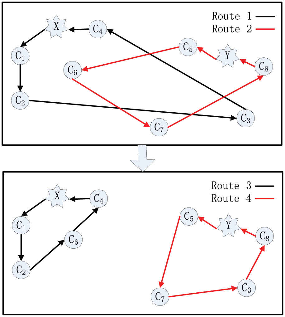
Comparison between the automobile maintenance parts delivery problems before and after in chain mode.

Based on a simple example, it is assumed that there are two automobile maintenance parts depots (X and Y) and eight automobile maintenance stations as customers (c₁, c₂, c₃, c₄, c₅, c₆, c₇, c₈). Originally, company X is responsible for serving four automobile maintenance stations (c₁, c₂, c₃, c₄), while company Y is responsible for serving the other four automobile maintenance stations (c₅, c₆, c₇, c₈). The delivery routes (routes 1 and 2) can be seen in Figure 1 (originally).

When all of the companies X, Y and the automobile maintenance stations (c₁, c₂, c₃, c₄, c₅, c₆, c₇, c₈) are in the chain operation mode, the eight customers are served by the two depots collaboratively. Then the new delivery routes (routes 3 and 4) can be acquired, which can be seen in Figure 1 (subsequently). And it is obvious that the length of route 3 + route 4 < route 1 + route 2. Therefore, the collaborative method in chain operation mode can effectively reduce delivery costs.

In addition, to meet timely service for customers and improve the service level, each automobile maintenance station provides its time window requirements. Thus, the automobile chain maintenance enterprise attempts to consider how to serve the stations collaboratively from these depots to minimize the delivery cost while meeting the requirements of automobile maintenance stations. From a modeling viewpoint, the automobile maintenance parts delivery problem in the chain operation mode can be thought of as a multi-depot vehicle routing problem with time windows (MDVRPTW).

MDVRPTW is an extension of multi-depot vehicle routing problem (MDVRP) and vehicle routing problem with time windows (VRPTW), which is also a non-deterministic polynomial-time (NP)-hard problem. As for the MDVRP, there have been many literatures which mentioned it. Mirabi et al.² presented a hybrid heuristic searches and improvement techniques to improve the performance of the algorithm. Yu et al.³ aimed to solve MDVRP using an improved ant colony optimization (ACO), where a coarse-grain parallel strategy, ant-weight strategy, and mutation operation are used to improve the searching ability of ACO. Ho et al.⁴ attempted to solve MDVRP with a hybrid genetic algorithm. Tu et al.⁵ proposed a Voronoi diagram–based meta-heuristic to solve MDVRP. There have also been many literatures which mentioned VRPTW. Yanik et al.⁶ developed a hybrid meta-heuristic approach using a genetic algorithm for vendor selection and allocation and a modified savings algorithm for the capacitated VRP with multiple pickup, single delivery, and time windows. Lin⁷ addressed a pickup and delivery problem with time window constraints, using a two-stage heuristic and two types of delivery resources which allows for coordination. Lai and Cao⁸ constructed a general mixed-integer programming model of vehicle routing problem with simultaneous pickups and deliveries and time windows (VRP-SPDTW) and proposed an improved differential evolution (IDE) algorithm for solving the problem of optimally integrating forward and reserve logistics for cost saving and environmental protection. Derigs and Döhmer⁹ proposed that the indirect local search heuristics with greedy decoding are not only flexible and simple but also gives results which are competitive with state-of-the-art vehicle routing problem with pickup and delivery and time windows methods. Wang and Meng¹⁰ formulated Liner shipping network problem as a mixed-integer non-linear non-convex programming model and proposed a column generation–based heuristic method for solving this problem. Ding et al.¹¹ presented a hybrid ACO by adjusting pheromone approach and introducing a disaster operator for solving the vehicle routing problem with time windows. As for MDVRPTW, the present research is less although it has recently received growing concern. Dondo and Cerdá¹² attempted to solve MDVRPTW by a hybrid local search improvement algorithm. Liu¹³ developed an improved adaptive genetic algorithm based on the artificial bee colony algorithm to solve MDVRPTW. Zhen and Zhang¹⁴ proposed a hybrid meta-heuristic algorithm to solve MDVRPTW. Wen and Meng¹⁵ developed an improved particle swarm optimization (PSO) to deal with MDVRPTW efficiently. In one word, the heuristic algorithm is often the first choice for solving this kind of complicated problems.

ACO is one of the most famous meta-heuristic algorithms and was initially used on the classical traveling salesman problem. The fundamental idea of ACO is to imitate the cooperative behavior of real ant colonies searching for the food. Pheromone, an aromatic essence, is left by real ants to communicate information concerning food sources. Instead of traveling randomly, other ants are attracted to follow the pheromone trails. Over the time, the path with more passing ants gets more deposited pheromone. At the same time, the pheromone trails evaporate and lose its attraction over time. The pheromones trails will disappear unless there are more ants to reinforce them. It is obvious that magnitude of the evaporation in longer path is higher than deposition in the shorter path. The ants on the shortest path lay pheromone trails faster, so the pheromone trail on this path increases up gradually. ACO, proposed by Dorigo et al.,¹⁶ has been successfully applied to many classic combinatorial optimization problems.^17–24 These successful applications for optimizing real-world problems motivated us to apply the ACO algorithm to solve the automobile chain maintenance parts delivery problem in this article.

The focus of this article is to solve a real-life delivery problem, the automobile chain maintenance parts delivery problem, which can be thought of as a MDVRPTW from a modeling viewpoint. Due to the complexity of automobile chain maintenance part delivery, the virtual center depot is used to simplify this problem, and then, improved ant colony optimization (IACO), a meta-heuristic, is applied to solve it. Thus, the remainder of this article is organized as follows. In section “Problem description,” we describe the automobile chain maintenance parts delivery problem and how the virtual center depot is used to simplify it. Section “An improved ACO for automobile chain maintenance parts delivery problem” presents the IACO algorithm and some improved strategies. Some computational results are discussed in section “Numerical analysis,” and finally, conclusions are provided in section “Conclusion.”

Problem description

Automobile chain maintenance parts delivery problem

The automobile chain maintenance parts delivery problem is described as follows: there are M automobile maintenance parts depots, each of which owns K_i vehicles with the capacity of w (i = 1, …, M), and all of which are responsible for services for n automobile maintenance stations; the demand of automobile maintenance station i is q_i (i = 1,…, n), and the total demand of each route does not exceed the vehicle capacity Vi,q_i < Vi. [a_i, b_i] is the time range that the automobile maintenance station i demands. The distance between two automobile maintenance stations or between automobile maintenance stations and delivery points is described as the vertex set, C, which is partitioned into two subsets: C_d = {c₁, …, c_H} is the set of automobile parts maintenance depots, and C_c = {c_H_+ 1, …, c_H_+ N} is the set of automobile maintenance stations. Each automobile maintenance station c_i ∈ C_c is associated with a non-negative demand q_i to be delivered and each depot c_h ∈ C_d is associated with a demand q_h = 0. Each automobile maintenance station can be served by only one vehicle from any depot. To avoid a vehicle passing two or more depots, we assume d_kl = ∞(c_k, c_l∈ C_d).The distance matrix is a real symmetric one, satisfying the triangle inequality principle, which is c_ik ≤ c_ij + c_jk. Each vehicle can serve several automobile maintenance stations whose demands must not overpass the transportation capacity of this vehicle. All vehicles start from one automobile parts maintenance depot, which it must return to.

Thus, the model of the automobile chain maintenance parts delivery problem is described as follows

min Z = \sum_{i = 0}^{n} \sum_{j = 0}^{n} \sum_{k = 0}^{K_{m}} \sum_{m = 0}^{M} C_{ij} x_{ij}^{mk}

(1)

\sum_{k = 1}^{K_{m}} \sum_{j = 1}^{N} x_{ij}^{mk} \leq K_{m} for i = m \in {N + 1, N + 2, \dots, N + M}

(2)

\sum_{j = 1}^{N} x_{ij}^{mk} = \sum_{j = 1}^{N} x_{ji}^{mk} \leq 1 for i = m \in {N + 1, N + 2, \dots, N + M}; k \in {1, 2, \dots, k_{m}}

(3)

\sum_{j = 1}^{N + M} \sum_{m = 1}^{M} \begin{matrix} \sum_{k = 1}^{K_{m}} x_{ij}^{mk} = 1 & for \begin{matrix} i \in {1, \dots, N} \end{matrix} \end{matrix}

(4)

\sum_{j = 1}^{N + M} \sum_{m = 1}^{M} \begin{matrix} \sum_{k = 1}^{K_{m}} x_{ij}^{mk} = 1 & for \begin{matrix} j \in {1, \dots, N} \end{matrix} \end{matrix}

(5)

\sum_{i = 1}^{N} q_{i} \sum_{j = 1}^{N + M} x_{ij}^{mk} \leq q_{mk} for m \in {N + 1, N + 2, \dots, N + M}; k \in {1, 2, \dots, k_{m}}

(6)

\sum_{j = N + 1}^{N + M} x_{ji}^{mk} = \sum_{j = N + 1}^{N + M} x_{ij}^{mk} = 0 for i = m \in {N + 1, N + 2, \dots, N + M}; k \in {1, 2, \dots, k_{m}}

(7)

E T_{i} \leq t_{i} + w_{i} \leq L T_{i} i = 1, 2, \dots, n

(8)

where

x_{ij}^{mk} = {\begin{matrix} 1 & the link from automoblie maintenance station i to j is visited by vehicle k from depot m \\ 0 & otherwise \end{matrix}

C_ij in formula (1) stands for the costs from automobile maintenance station i to j, it is the delivery distance from automobile maintenance station i to j; k is the number of vehicles; m is the number of automobile parts maintenance depots; q_mk is the capacity of vehicle k from depot m; K_m is the maximum number of vehicles at depot m; and k_m is vehicle k from depot m. The objective of the automobile chain maintenance parts delivery problem is to minimize the total delivery cost (distance or time spent) in serving all automobile maintenance stations within time windows. There are several constraints that are as follows.

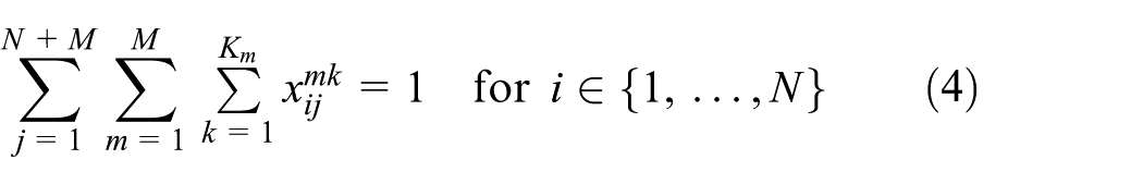
Formula (2) ensures that the number of vehicles does not exceed the maximum K_m. Formula (3) makes sure that each vehicle starts and ends at the same depot. Formulas (4) and (5) assume that each automobile maintenance station can be served exactly by one vehicle. Formula (6) assumes that the quantity of parts in a vehicle cannot exceed its capacity. Formula (7) constraint guarantees that there are no connections between these depots. Formula (8) ensures that each automobile maintenance station is served within the predefined time range. [ET_i, LT_i] is the time window of automobile maintenance station C_i. ET_i is the beginning of the arrival time of automobile maintenance station C_i’s demand and LT_i is the ending of the arrival time of automobile maintenance station C_i’s demand.

Automobile chain maintenance parts delivery problem with virtual center depot

Generally, the automobile maintenance parts delivery problem can be recognized as a MDVRPTW. And it is more difficult to solve MDVRPTW compared with the VRPTW with single depot (SDVRPTW) even for relatively small-sized instances. Thus, it is extremely time-consuming for solving the automobile chain maintenance parts delivery problem to optimality. In order to simplify MDVRPTW for attaining optimization results in an acceptable time, a virtual center depot is assumed and all the vehicles have to start from and end at the virtual center depot. The actual depots can be considered as the accesses of the “virtual” depot. Therefore, with the multiple fixed accesses, the MDVRPTW can be transformed into the SDVRPTW.

First, a virtual central depot c₀ is added. And its distances to the N automobile maintenance stations and H actual depots are, respectively, assumed as ∞ and 0. The route of each vehicle starts from the virtual central depot through one actual depot to customers and returns through the same actual depot to the virtual depot. At the same time, it is without exceeding the capacity constraints of each vehicle, the automobile maintenance stations are served within the predefined time windows. So the problem is transferred to multi-depot vehicle routing problem with the virtual central depot (V-MDVRPTW), which is similar to a SDVRPTW. Figure 2 describes an example of V-MDVRPTW with the same automobile maintenance stations and actual depots from Figure 1. In addition, all other constraints from the standard MDVRPTW still apply.

Figure 2.

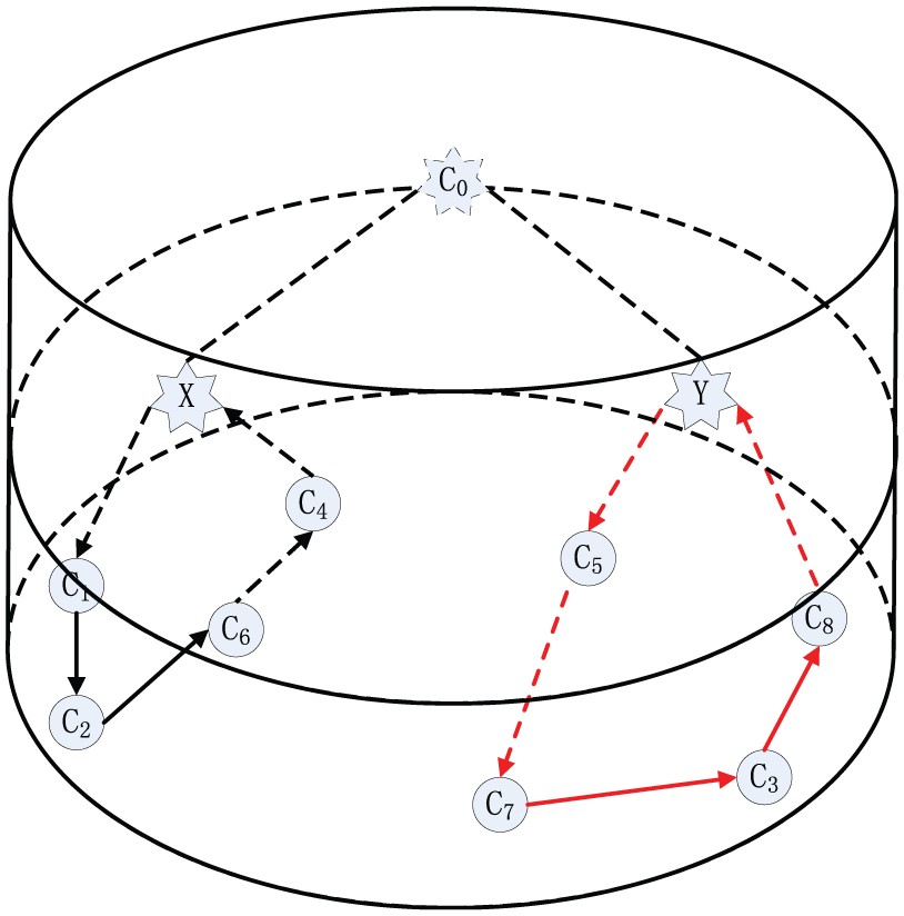
An example of V-MDVRPTW.

An improved ACO for automobile chain maintenance parts delivery problem

The solution of the V-MDVRPTW is to find a set of minimum cost routes in order to facilitate delivery from the virtual central depot through the H actual depots to a number of customer locations while the customers are served within the predefined time windows. It is very similar to food-seeking behaviors of ant colonies in nature. If the virtual central depot is considered as the nest, the actual depots are considered as the entries of nest, and customers are considered as the food, solving V-MDVRPTW can be described as the searching processes that starting from the nest through an entry to food within the predefined time windows.

The improved strategy of IACO

Although a lot of successful applications of ACO for optimizing real-world problems have been published, there are still some limits of the ACO in practice, such as easily getting trapped in local optimal solution, too much computational time spent to obtain the best solution, and great difficulty in adjusting the parameters to achieve the good performance. In order to avoid these above limits, an improved ACO for the V-MDVRPTW is proposed in this article. The improved strategy of IACO is as follows.

Saving algorithm applied in the generation of solutions

As a strong coupling algorithm, the ACO has the characteristic of combination with other heuristics. In order to improve the convergence speed, the saving algorithm is combined with the ACO.

The saving algorithm is one of the most widely known algorithms, which was proposed by Clarke and Wright.²⁵ It can be seen from Figure 3 that this algorithm is a very simple and efficient. Each customer is initially assigned to a separate route as shown in Figure 3(a). As shown in Figure 3(b), it is obvious that a saving can be obtained by combining the two customers C_i and C_j on the same route. For the result shown in Figure 3(c), the savings are determined by equation (9)

s_{ij} = d_{0 i} + d_{0 j} - d_{ij}

(9)

where d_0i denotes the distance between the depot 0 and the customer C_i. d_0j denotes the distance between the depot 0 and the customer C_j. d_ij denotes the distance between the customer C_i and C_j. The best combination is then chosen and the procedure is iterated.

Figure 3.

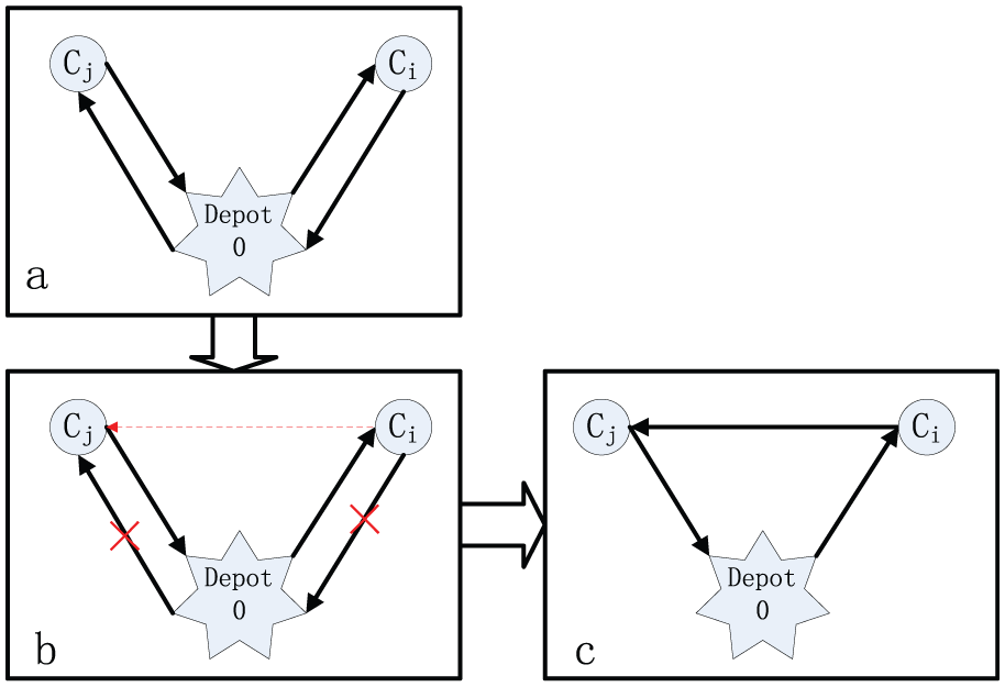
Illustration of the saving algorithm: (a) Initial, (b) Saving, and (c) Result.

In the period of initializing, the repeated counter is defined as n_c = 0, m ants are placed on the virtual center depot, and a candidate list is made. In order to extend the combination scale and obtain the feasible solution more easily, m can be given a larger value and the number of ants can be increased unless all customers are visited in the search process.

In IACO for MDVRPTW, the decision-making about combining customers is based on a probabilistic rule taking into account both the visibility and the pheromone information on an edge. Thus, to select the next customer j, the ant uses the following probabilistic formula

p_{ij} (k) = {\begin{matrix} \frac{τ_{ij}^{α} \times η_{ij}^{β} \times μ_{ij}^{γ}}{\sum_{h \notin tab u_{k}} τ_{ih}^{α} \times η_{ih}^{β} \times μ_{ij}^{γ}} & q \leq p_{t} and j \notin tab u_{k} \\ 0 & otherwise \end{matrix}

(10)

where, p_ij(k) is the probability of choosing to combine customers i and j on the route, τ_ij the pheromone density of edge (i, j), η_ij the visibility of edge (i, j), and µ_ij the saving value on the basis of saving algorithm. α, β, and γ are the relative influence of the pheromone trails, the visibility values, and the saving values, respectively; tabu_k (k = 1,2, …, m) is the set of the infeasible nodes for the k_th ant, such as the nodes which have been visited by the k_th ant or the nodes which are not available within the time windows. q is a value chosen randomly with uniform probability in the interval [0, 1]. P_t(0 < P_t ≤ 1) interpreted as the definite election probabilities is initiated as p₀ = 1 and is dynamically adjusted with the evolutionary process.

Mutation operation

To overcome the weakness of ACO tending to get trapped in local optimal solution, the mutation operation can be used to increase the solution space in a lot of research fields.^17,26,27 It has empirically shown that the mutation operation can help the ACO to avoid premature convergence. In this article, there are two kinds of mutation operations which are applied to produce a new solution that is not far different from the original one.

One is called the depot mutation operation, which is said to choose a route and a neighboring actual depot, and then to change the actual depot to become a new route. And the other is called the customer mutation operation, which is said to choose a route and a neighboring customer, and then to change the customer into the chosen route. Figures 4 and 5 show two examples of these two kinds of mutation operations, respectively.

Figure 4.

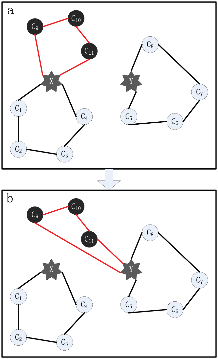
Illustration of the depot mutation operation: (a) Select a route and a neighbor depot and (b) Mutation operation.

Figure 5.

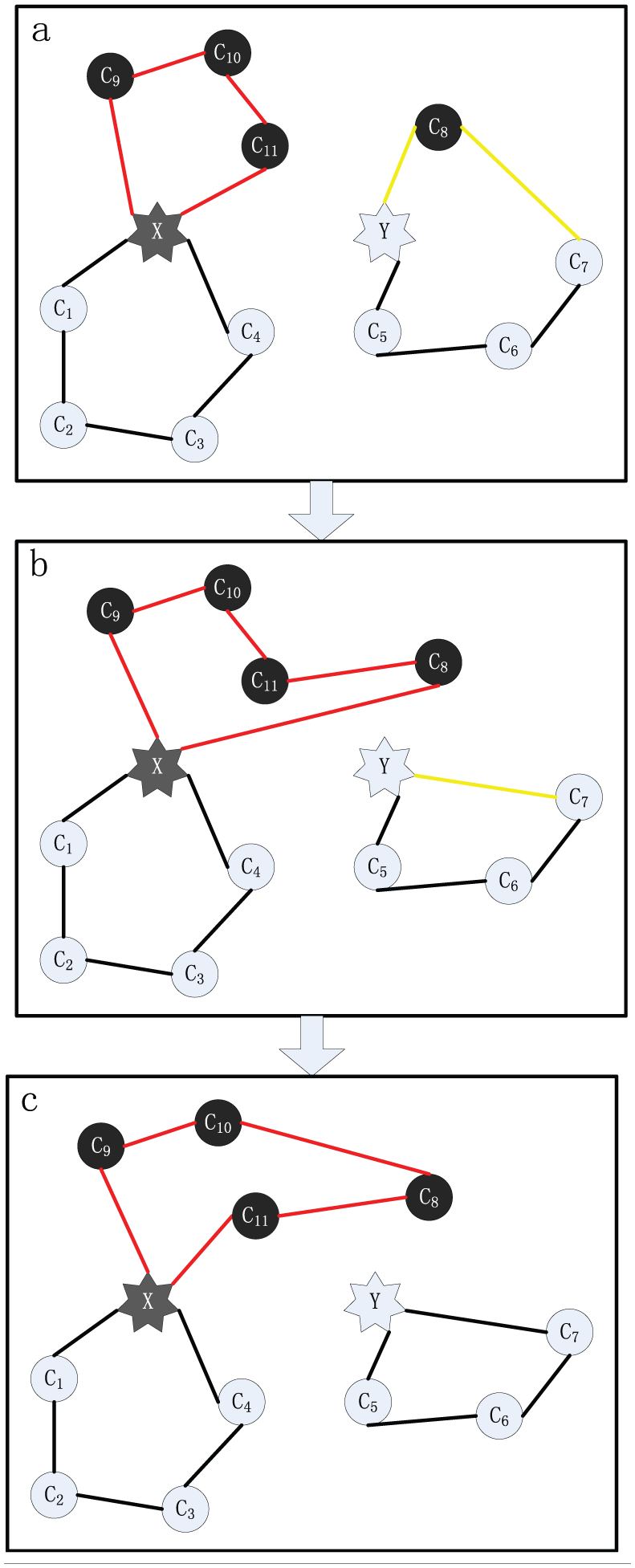
Illustration of the customer mutation operation: (a) Select a route and a neighbor depot, (b) New solution, and (c) Local optimality.

As shown in Figure 4, there are generally two steps in the depot mutation operation. First, a route and a neighboring actual depot are selected as shown in Figure 4(a). Then, a new solution is produced by replacing the depot of the selected route by the neighboring actual depot, as shown in Figure 4(b).

As shown in Figure 5, there are generally three steps in the customer mutation operation.

First, a route and a neighboring customer are selected as shown in Figure 5(a).

Second, the two edges that are linked to the neighboring customer are deleted. And the other customer(s) or the depot in the old route that links to the deleted edges is directly linked. So a new shorter route is produced. At the same time, a new solution is produced by linking the neighboring customer to the last customer and the depot of the route selected in the first step, as shown in Figure 5(b).

Finally, if the mutation operations violate the vehicle capacity constraints or time window constraints, the route amounts should be added to fix the resultant capacity violations. Furthermore, in order to ensure the local optimality of each route in the new solution, the 2-opt exchange is applied to search the whole customer sequence by assessing all possible pairwise exchanges of the customer locations in a route.

Improvement strategies of pheromone information updating

As an adaptive learning technique,²⁸ the updating of pheromone trails plays an important role in the ACO, which reflects the ant’s performance and the quality of the solutions found. There are two parts of the updating of pheromone. First, in order to ensure that no one path becomes too dominant, the natural evaporation of pheromone is simulated. Then the pheromone increment happens in every visited edge.

Considering the important role of the pheromone information updating, some improvement strategies are applied to avoid both becoming trapped in local optimal solution and obtaining premature convergence, meanwhile owning an acceptable convergence speed.

First, simulation of the natural evaporation of pheromone is conducted to reduce the amount of pheromone on each segment in the period of pheromone decrements of ACO. This is done with the following pheromone updating equation

τ_{ij}^{new} = ρ \times τ_{ij}^{old} + \sum_{h} \sum_{k} Δ τ_{h}^{k} (i, j) ρ \in (0, 1)

(11)

where, $τ_{ij}^{new}$ is the pheromone on the link (i, j) after updating; $τ_{ij}^{old}$ is the pheromone on the link (i, j) before updating; $Δ τ_{h}^{k} (i, j)$ is the pheromone increments on the k_th route through the h_th actual depot on edge (i, j); ρ is the constant that controls the speed of evaporation; and k is the number of the route.

Because of the existence of the trail evaporation coefficient 1 − ρ, the pheromone of the edges never visited by artificial ants should gradually decrease and becomes close to 0, which makes the global optimization capability of the ACO to reduce. It is obvious that the larger the evaporation coefficient, the better the global optimization capability, but the convergence speed of the algorithm will be slowed down at the same time. Due to this weakness, there are more difficulties for the traditional ACO algorithm to solve large-scale problems. Therefore, in this article, a dynamic evaporation coefficient 1 − ρ value is adopted rather than a constant value.

Second, there are some strategies updating the pheromone increments. And the most popular strategies are ant-density, ant-quantity, and ant-cycle. Too much time is wasted by a large amount of invalid searches, because some of them omit global information, while the others omit local information. Thus, ant-weight strategy taking into account both the global and the local information has been adopted to update the increased pheromone in this article. Specifically, the strategy is written as

Δ τ_{h}^{k} (i, j) = {\begin{matrix} \frac{Q}{L} \times \frac{L - L_{h}}{(H - 1) \times L} \times \frac{L_{h} - f_{h}^{k}}{(n_{h} - 1) \times L_{h}} & \begin{matrix} if link (i, j) on the k_{th} route through \\ the h_{th} actual depot \end{matrix} \\ 0 & otherwise \end{matrix}

(12)

where Q is a constant; L is the total length of all routes in the solution, that is, $L = \sum_{h} L_{h}$ ; L_h is the total length of all routes through the h_th actual depot in the solution, that is, $L_{h} = \sum_{k} f_{h}^{k}$ ; $f_{h}^{k}$ is the length of the k_th route through the h_th actual depot in the solution; and n_h is the number of the routes through the h_th actual depot and $n_{h} \geq 1$ .

Based on ant-weight strategy, the total pheromone increments on all edges that the solution covers are equal to Q/L. The proportion of the pheromone increments shared by the routes through the h_th actual depot to the total pheromone increments is equal to $(L - L_{h}) / (H - 1) \times L$ .

According to the same principle, the pheromone increments on each edge on a route through the h_th actual depot are related to the contribution of the edge to the route. That is, the pheromone increment proportion of the edge (i, j) is equal to $(L_{h} - f_{h}^{k}) / ((n_{h} - 1) \times L_{h})$ .

In this way, both the global and the local information are taken into account, and the learning capacity of the algorithm from past searches is improved, which enhances the efficiency.

Finally, inspired by the idea of MAX–MIN ant system, $τ_{max}$ and $τ_{min}$ as the maximum and minimum pheromone trails are predefined to limit all pheromone trails to satisfy $τ_{min} \leq τ_{ij} \leq τ_{max}$ . At every edge, huge difference between the maximum and minimum pheromone trails may lead to premature convergence of the search. In case the pheromone trails differ greatly, the idea of computing average pheromone trails between τ_ij and τ_max is adopted to avoid premature convergence. Meanwhile, the pheromone trails are deliberately initialized to τ_max, which helps to find a better solution at the beginning of the search. After pheromone trails are dynamically updated, τ_ij is replaced by τ_max when τ_ij > τ_max, or by (τ_min + τ_max)/2 when τ_ij > τ_min.

Steps of the IACO

The steps of the IACO for solving the MDVRPTW model can be described as follows:

Step 1. Initialize every controlling parameter, assume the best solution L_global based on the actual data, define the repeated counter as n_c = 0, put m ants on the depots, and make a tabu list. M should be given a certain value which is large enough in order to obtain the feasible solution more easily. M should be increased unless the present number of ants can ensure all customers are visited in the search process.

Step 2. According to the probabilistic formula (1), the ant selects the next customer one by one. And the solution will be generated as the strategy described in section “Saving algorithm applied in the generation of solutions.”

Step 3. Go back to step 2 if the total amount of searching ants is smaller than m, and the remaining ants will continue searching; otherwise, go to step 4.

Step 4: Compute the solution L_k of every ant, set $L_{local} = \sum_{k = 1}^{m} L_{k}$ as the local optimal solution.

Step 5. Perform mutation operation with 2-opt exchange as the strategy described in section “Mutation operation.” If the solution L_opt < L_local and the new route satisfy the constraints of capacity of the vehicle and time windows, set L_local = L_opt.

Step 6. All the pheromone trails are dynamically updated as the strategy described in section “Improvement strategies of pheromone information updating.”

Step 7. Compare L_local with L_global. If L_local < L_global, set L_global = L_local.

Step 8. When the direction of evolution has been basically determined after several generations of evolution, the p_t and ρ should be adaptively adjusted as follows

p_{t} = {\begin{matrix} 0.95 p_{t - 1} & if 0.95 p_{t - 1} \geq p_{min} \\ p_{min} & otherwise \end{matrix}

(13)

ρ_{n} = {\begin{matrix} 0.95 ρ_{t - 1} & if 0.95 ρ_{t - 1} \geq ρ_{min} \\ ρ_{\min} & otherwise \end{matrix}

(14)

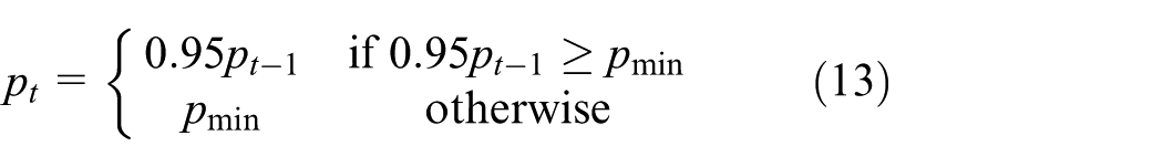
where p_min as the minimum defined in evolutionary process is used to ensure that the definite choosing chance could be achieved even if p_t is too small. ρ_min as the minimum defined in the evolutionary process is used to avoid a too slow convergence speed when ρ is too small.

Step 9. If n_c is bigger than the maximum, then the algorithm is completed. Otherwise, go back to step 2 and repeat the above steps.

Numerical analysis

This article attempts to use an improved ACO algorithm to solve the automobile chain maintenance parts delivery problem, which is a real-life delivery problem. Since there are several depots with time windows in this real-life delivery problem, for comparisons, some well-known benchmark problems of MDVRP are applied to examine the performance and feasibility of the IACO. Then, the IACO is used to solve the automobile chain maintenance parts delivery problem. The two examples will be described, respectively, as follows.

The classical MDVRPTW

The benchmark problems of MDVRPTW from literatures^29,30 are selected to examine the performance of the proposed IACO in this article. These problems include the number of available vehicles, Euclidean distances among customers and normalized vehicle speeds making traveling times, and Euclidean distances numerically identical. Furthermore, time windows are regarded as hard constraints and service times are independent of customer requirements. The selected objective is the minimization of the total distance cost. The most important characteristics of these problems are presented in Table 1 briefly.

Table 1.

The information of the test problems.

No.	H	n	Q	m
P01	4	48	200	2
P02	4	96	195	3
P03	4	144	150	4
P04	4	192	185	5
P05	4	240	180	6
P06	4	288	175	7
P07	6	72	200	2
P08	6	144	190	3
P09	6	216	180	4
P10	6	288	170	5
P11	4	48	200	1
P12	4	96	195	2
P13	4	144	150	3
P14	4	192	185	4
P15	4	240	180	5
P16	4	288	175	6
P17	6	72	200	1
P18	6	144	190	2
P19	6	216	180	3
P20	6	288	170	4

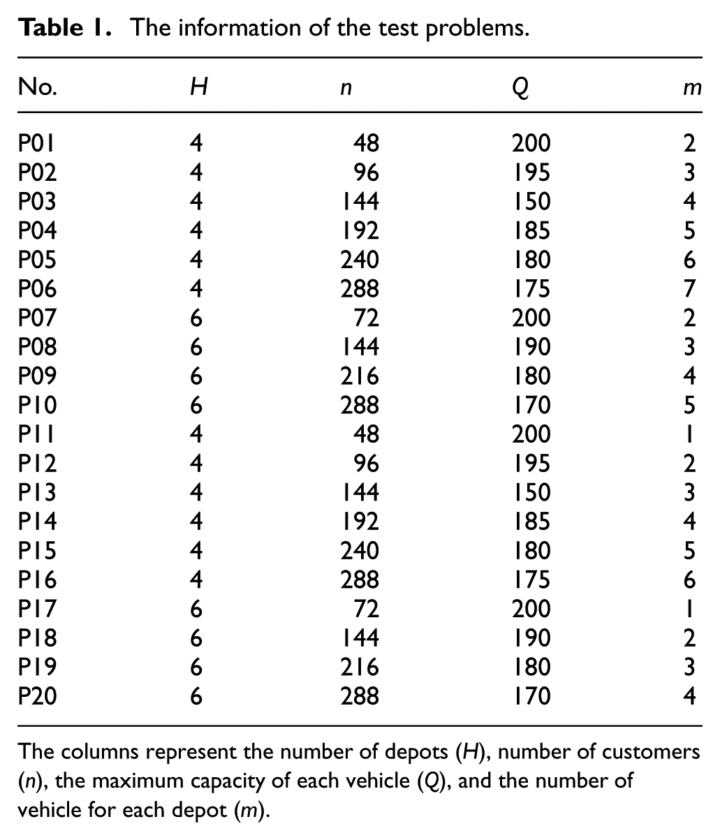
The columns represent the number of depots (H), number of customers (n), the maximum capacity of each vehicle (Q), and the number of vehicle for each depot (m).

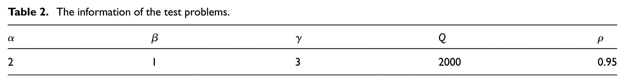
In this article, VC++ 2010 is used to achieve the IACO, and operating environment is the Pentium IV 2.93 GHz processor and 4 GB for the Windows platform. The parameters in the IACO (Table 2) are estimated through simulation.

Table 2.

The information of the test problems.

α	β	γ	Q	ρ
2	1	3	2000	0.95

In order to test the performance of the algorithm, the results of the proposed IACO algorithm are compared with variable neighborhood search (VNS), TS new,²⁹ and high-level relay hybrid meta-heuristic method (HL-HM).³⁰ These instances and the best known solutions are available at http://www.bernabe.dorronsoro.es/vrp/. Table 3 is the result of these algorithms for solving the MDVRPTW.

Table 3.

Computational results using IACO algorithm and some well-known published results.

No.	Best-known results	VNS	TS new	HL-HM	ACO	IACO
P01	1083.98	1083.98	1074.12	1101.8	1086.85	1080.58
P02	1763.07	1763.07	1762.21	1762.21	1768.96	1763.07
P03	2408.42	2374.36	2373.65	2408.42	2655.38	2374.35
P04	2958.23	2858.20	2815.48	2958.2	3605.49	2952.99
P05	3134.04	3040.84	2993.94	3029.65	3785.49	3034.27
P06	3904.07	3758.36	3629.72	3758.36	4356.26	3758.36
P07	1423.35	1422.65	1418.22	1418.22	1464.67	1418.22
P08	2150.22	2103.89	2096.73	2103.89	2446.31	2107.15
P09	2833.80	2783.95	2730.54	2737.82	3467.28	2734.18
P10	3717.22	3577.28	3499.56	3577.28	4241.06	3577.28
P11	1031.49	1005.73	1005.73	1005.73	1038.67	1006.04
P12	1500.48	1487.64	1472.76	1478.51	1496.43	1475.37
P13	2020.58	2014.02	2001.83	2014.02	2285.63	2007.37
P14	2247.72	2221.17	2215.51	2202.08	2686.86	2214.17
P15	2509.75	2494.82	2465.25	2509.75	3258.39	2484.37
P16	2943.90	2939.20	2896.03	2896.03	3659.48	2895.18
P17	1250.09	1239.13	1236.24	1239.13	1312.67	1237.29
P18	1809.35	1796.21	1796.21	1796.21	2137.49	1796.21
P19	2310.92	2318.59	2292.45	2310.92	2784.83	2298.69
P20	3131.90	3079.73	3076.37	3079.73	3869.73	3077.48

IACO: improved ant colony optimization; VNS: variable neighborhood search; HL-HM: high-level relay hybrid meta-heuristic method; ACO: ant colony optimization.

From Table 3, it can be found that most results of the IACO algorithm are close to well-known best solutions. Even several solutions are better than the best solutions among these algorithms. The results indicate that the IACO algorithm is suitable for solving MDVRPTW.

The automobile chain maintenance parts delivery problem

It is verified by the benchmark problem that the IACO algorithm is suitable to solve MDVRPTW. A real-life routing problem solved by the IACO algorithm will be described in this section.

The spatial characteristics of Dalian in this real-life automobile chain maintenance parts delivery route problem can be described in Figure 6. It can be seen that there are several automobile maintenance parts depots and some maintenance stations in Dalian city. The letters (A, B, and C) represent three automobile maintenance parts depots in Dalian, and the numbers (1, 2, …, 39) stand for the 39 automobile maintenance stations in Dalian. The specific spatial information of the automobile maintenance parts depots and the automobile maintenance stations is shown in Tables 4 and 5, respectively. The core problem is how these automobile maintenance parts depots delivery the parts to the maintenance stations with the least cost.

Figure 6.

The location information of the automobile chain maintenance parts delivery route problem.

Table 4.

The information of automobile part suppliers.

Depots	A	B	C
Longitude	121.578	121.637	121.6
Latitude	38.959	38.9337	38.932
Vehicle number	3	3	3

Table 5.

The information of the automobile maintenance stations in Dalian.

Customers	1	2	3	4	5	6	7	8
Longitude	38.9072	38.9118	38.9489	38.876	38.9224	38.884	38.8939	38.9679
Latitude	121.608	121.574	121.567	121.548	121.601	121.639	121.584	121.519
Demand	10	24	20	12	10	12	10	38
Time	206–382	188–317	301–437	340–431	472–650	240–370	455–465	172–303
Customers	9	10	11	12	13	14	15	16
Longitude	38.9742	38.9796	38.9633	38.9758	38.8846	38.9184	38.9212	38.8919
Latitude	121.557	121.587	121.546	121.612	121.651	121.674	121.642	121.676
Demand	18	80	50	50	24	36	20	30
Time	151–288	188–317	126–226	164–259	339–476	225–327	433–562	340–431
Customers	17	18	19	20	21	22	23	24
Longitude	38.9156	38.8772	38.8846	38.9109	38.885	38.9124	38.9008	38.8987
Latitude	121.616	121.527	121.56	121.587	121.584	121.601	121.599	121.644
Demand	16	18	16	18	22	10	15	15
Time	154–317	301–437	239–354	184–306	433–562	478–614	472–563	381–551
Customers	25	26	27	28	29	30	31	32
Longitude	38.9149	38.9055	38.9263	38.9264	38.9276	38.9089	38.8646	38.8872
Latitude	121.636	121.666	121.658	121.638	121.619	121.63	121.626	121.7
Demand	15	60	30	20	28	20	16	18
Time	171–304	200–331	160–290	455–465	122–249	184–306	310–468	440–549
Customers	33	34	35	36	37	38	39
Longitude	38.8837	38.8766	38.9148	38.9687	38.9755	38.9404	38.8936
Latitude	121.546	121.564	121.66	121.59	121.513	121.577	121.623
Demand	20	13	20	60	22	40	10
Time	240–370	381–551	189–280	220–331	191–343	336–435	223–350

The length of vehicle routing should be based on the distance traveled by vehicles which should be measured based on the road network in practice. Thus, a method to measure the actual distance and construct the distance matrix is adopted in this article.^31,32 The process of how to transfer the actual route distances into the rectilinear distances will be described as follows.

First, calculate the route distance between two points. If there are several routes between the two points, the least length among them is considered as the route distance. Second, attain the distance matrix based on real road network. Finally, transfer the actual distance into the symmetric distance matrix.

In the real-life routing problem, the optimized objective is the least cost, while the automobile maintenance stations are served within the time windows and the vehicle capacity is 200. After the IACO continues calculating 10 times, the results are shown in Figure 7. It is can be seen that the results are very stable and the difference between the best optimum and the worst is less than 10%. It can be proved that this algorithm has an excellent convergence performance. Meanwhile, the computing time is from 220 to 300 s which is completely acceptable for a real-life problem. In one word, the proposed IACO can solve the real-life automobile chain maintenance parts delivery route problem in Dalian city with a remarkable optimization quality and acceptable computing time.

Figure 7.

Computing results of IACO after running 10 times.

The length of the optimized routes is 104.09 km. The result of the optimized routes is shown in Figure 8.

Figure 8.

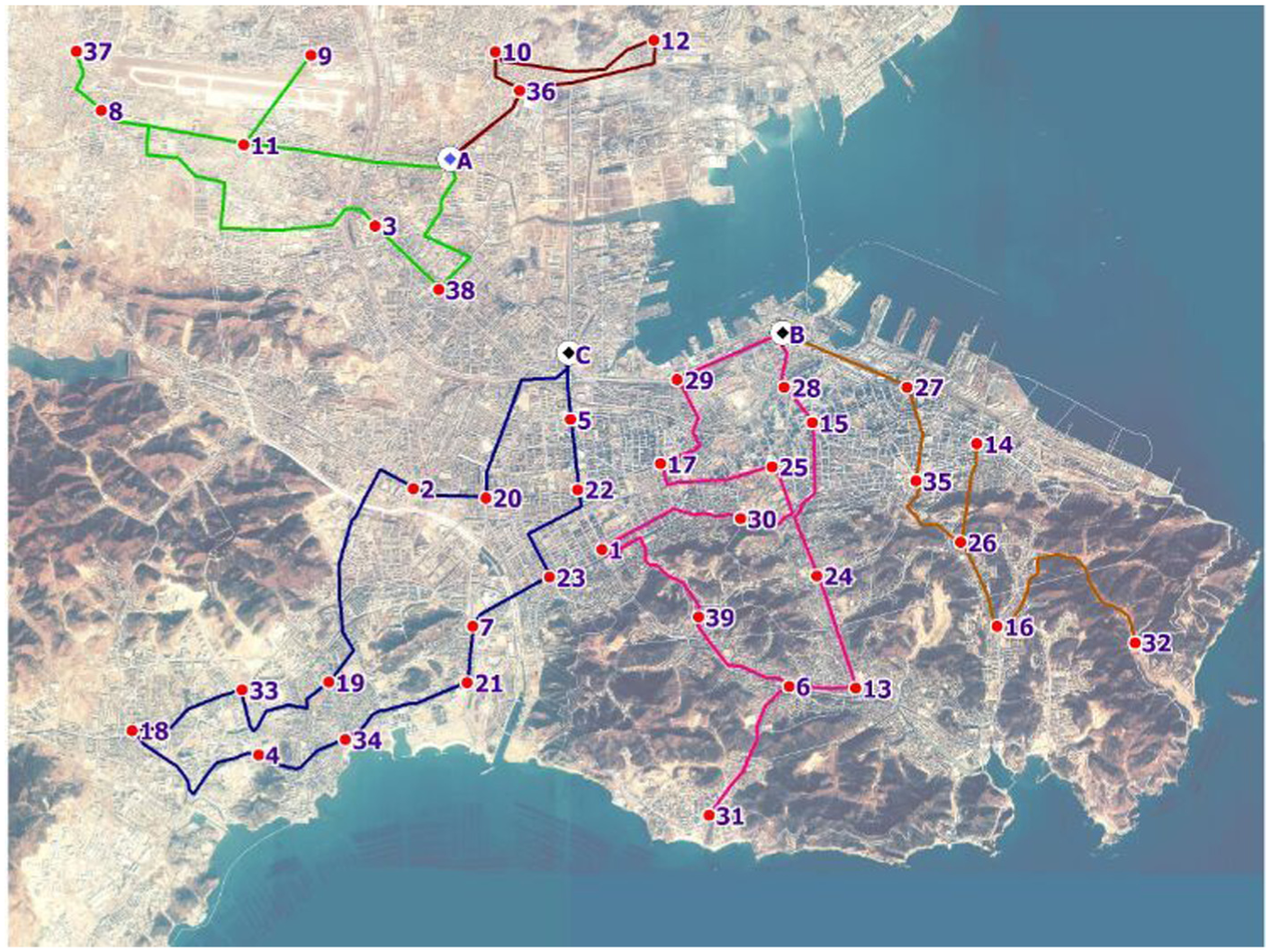
Distribution routes of the automobile chain maintenance parts delivery route problem based on IACO.

To examine the effectiveness of the proposed method in this article, the solution of the current situation (before operate in chain model) is compared with the optimized solution of the proposed method, which is seen in Table 6.

Table 6.

The number of vehicles and the total distance between the current situation and the proposed method.

	The number of vehicle	Total distance (km)
The current situation	9	132.13
The proposed method	4	104.09

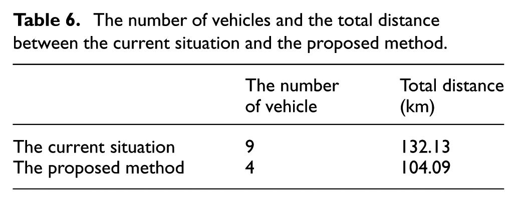
From Table 6, it is obvious that the total distance of the proposed model is shorter than the one from current situation. Furthermore, the number of vehicle is reduced. It is due to that the operation in chain model is more effective . And the improved ACO is an effective method to solve the automobile maintenance chain spare parts delivery route problem.

Conclusion

The objective of automobile chain maintenance parts delivery problem is to minimize the total delivery distance in serving all the maintenance stations in the city, and the time when the vehicle arrives at every maintenance station should be within the required time. Since the automobile chain maintenance parts delivery problem is difficult to be solved, virtual center depot is assumed and adopted to transfer MDVRPTW to VRPTW in this article, which can effectively reduce the complexity. Then an IACO is presented to solve automobile chain maintenance parts delivery problem. The computational results of the benchmark problems suggest that the proposed adaptive IACO is effective to solve MDVRPTW with an acceptable running speed. And the implementation of automobile chain maintenance parts delivery problem, in the design of delivery routes for several automobile maintenance part depots to serve some service stations within a time window in Dalian, can provide suitable results. Therefore, the proposed IACO can be considered as an effective method for the automobile chain maintenance parts delivery problem. And the results show that the automobile chain maintenance parts delivery problem proposed in this article can effectively integrate the smaller companies to improve their competitiveness and customer satisfaction by reducing the delivery and time cost.

However, in this article, both the transportation cost and the traveling time are only considered to correspond to the transportation distance. In fact, the transportation cost and the traveling time would be related to the traffic conditions (time-of-day, weather, and so on) in a real-life condition. Other aspects of the real-life problem so as to enhance the performance of the proposed methods will be considered in the further study.

Footnotes

Academic Editor: Gang Chen

Declaration of conflicting interests

The author(s) declared no potential conflicts of interest with respect to the research, authorship, and/or publication of this article.

Funding

The author(s) disclosed receipt of the following financial support for the research, authorship, and/or publication of this article: This work is partially supported by the grants from the National Natural Science Foundation of China 51578112, Humanity and Social Science Youth foundation of Ministry of Education of China 13YJCZH042, Specialized Research Fund for the Doctoral Program of Higher Education of China 20120041120018 and the Fundamental Research Funds for the Central Universities DUT16YQ104.

References

Yao

Gao

. An improved particle swarm optimization for carton heterogeneous vehicle routing problem with a collection depot. Ann Oper Res 2016; 242: 303–320.

Mirabi

Ghomi

SMTF

Jolai

Efficient stochastic hybrid heuristics for the multi-depot vehicle routing problem. Robot Cim: Int Manuf 2010; 26: 564–569.

Yang

Xie

JX.

A parallel improved ant colony optimization for multi-depot vehicle routing problem. J Oper Res Soc 2011; 62: 183–188.

GTS

. A hybrid genetic algorithm for the multi-depot vehicle routing problem. Eng Appl Artif Intel 2008; 21: 548–557.

Fang

. A bi-level Voronoi diagram-based metaheuristic for a large-scale multi-depot vehicle routing problem. Transport Res E: Log 2014; 61: 84–97.

Yanik

Bozkaya

Jouan de Kervenoael

A new VRPPD model and a hybrid heuristic solution approach for e-tailing. Eur J Oper Res 2014; 236: 879–890.

Lin

CKY

. A vehicle routing problem with pickup and delivery time windows, and coordination of transportable resources. Comput Oper Res 2011; 38: 1596–1609.

Lai

Cao

EB.

An improved differential evolution algorithm for vehicle routing problem with simultaneous pickups and deliveries and time windows. Eng Appl Artif Intel 2010; 23: 188–195.

Derigs

Döhmer

Indirect search for the vehicle routing problem with pickup and delivery and time windows. OR Spectrum 2008; 30: 149–165.

10.

Wang

Meng

Liner shipping network design with deadlines. Comput Oper Res 2014; 41: 140–149.

11.

Ding

Sun

. An improved ant colony optimization and its application to vehicle routing problem with time windows. Neurocomputing 2012; 98: 101–107.

12.

Dondo

Cerdá

A hybrid local improvement algorithm for large-scale multi-depot vehicle routing problems with time windows. Comput Chem Eng 2009; 33: 513–530.

13.

Liu

CY.

An improved adaptive genetic algorithm for the multi-depot vehicle routing problem with time window. J Network 2013; 8: 1035–1042.

14.

Zhen

Zhang

. A hybrid metaheuristic algorithm for the multi-depot vehicle routing problem with time windows. In: Proceedings of the international conference on networks security, wireless communications and trusted computing (NSWCTC ‘09), Wuhan, China, 25–26 April 2009, vol. 2, pp.798–801. New York: IEEE.

15.

Wen

Meng

. An improved PSO for the multi-depot vehicle routing problem with time windows. In: Proceedings of the Pacific-Asia workshop on computational intelligence and industrial application, 2008 (PACIIA ‘08), Wuhan, China, 19–20 December 2008, vol. 1, pp.852–856. New York: IEEE.

16.

Dorigo

Maniezzo

Colorni

Ant system: optimization by a colony of cooperating agents. IEEE T Syst Man Cy B 1996; 26: 29–41.

17.

Yang

Yao

An improved ant colony optimization for vehicle routing problem. Eur J Oper Res 2009; 196: 171–176.

18.

Yang

ZZ.

An ant colony optimization model: the period vehicle routing problem with time windows. Transport Res E: Log 2011; 47: 166–181.

19.

Matos

Oliverira

RC.

An experimental study of the ant colony system for the period vehicle routing problem. Lect Notes Comput Sc 2004; 3172: 286–293.

20.

Tan

Zhuo

Zhang

. Ant colony system for optimizing vehicle routing problem with time windows (VRPTW). In: Proceedings of the international conference on intelligent computing, Kunming, China, 16–19 August 2006, vol. 2, pp.209–215. Berlin: Springer.

21.

Zhu

Zhen

. Hybrid ant colony algorithm based on vehicle routing problem with time windows. In: Proceedings of the WASE international conference on information engineering, Taiyuan, China, 10–11 July 2009, vol. 2, pp.50–53. New York: IEEE.

22.

Bell

McMullen

PR.

Ant colony optimization techniques for the vehicle routing problem. Adv Eng Inform 2004; 18: 41–48.

23.

Schoonderwoerd

Holland

Bruten

. Ant-based load balancing in telecommunications networks. Adapt Behav 1997; 5: 169–207.

24.

Albritton

McMullen

PR.

Optimal product design using a colony of virtual ants. Eur J Oper Res 2007; 176: 498–520.

25.

Clarke

Wright

JW.

Scheduling of vehicles from a central depot to a number of delivery points. Oper Res 1964; 12: 568–581.

26.

Yao

. Merged automobile maintenance part delivery problem using an improved artificial bee colony algorithm. Sci Iran 2015; 22: 1258–1270.

27.

Yao

Chen

Cao

. Short-term traffic speed prediction for an urban corridor. Comput-Aided Civ Inf. Epub ahead of print 21 July 2016. DOI: 10.1111/mice.12221.

28.

Yue

Wei

Adaptive sliding-mode control for two-wheeled inverted pendulum vehicle based on zero-dynamics theory. Nonlinear Dynam 2014; 76: 459–471.

29.

Polacek

Hartl

Doerner

. A variable neighborhood search for the multi depot vehicle routing problem with time windows. J Heuristics 2004; 10: 613–627.

30.

Noori

Ghannadpour

SF.

High-level relay hybrid metaheuristic method for multi-depot vehicle routing problem with time windows. J Math Model Algorithm 2012; 11: 159–179.

31.

Yao

. Transit network design based on travel time reliability. Transport Res C: Emer 2014; 43: 233–248.

32.

Kong

Sun

. A bi-level programming for bus lane network design. Transport Res C: Emer 2015; 55: 310–327.

No.	H	n	Q	m
P01	4	48	200	2
P02	4	96	195	3
P03	4	144	150	4
P04	4	192	185	5
P05	4	240	180	6
P06	4	288	175	7
P07	6	72	200	2
P08	6	144	190	3
P09	6	216	180	4
P10	6	288	170	5
P11	4	48	200	1
P12	4	96	195	2
P13	4	144	150	3
P14	4	192	185	4
P15	4	240	180	5
P16	4	288	175	6
P17	6	72	200	1
P18	6	144	190	2
P19	6	216	180	3
P20	6	288	170	4

No.	H	n	Q	m
P01	4	48	200	2
P02	4	96	195	3
P03	4	144	150	4
P04	4	192	185	5
P05	4	240	180	6
P06	4	288	175	7
P07	6	72	200	2
P08	6	144	190	3
P09	6	216	180	4
P10	6	288	170	5
P11	4	48	200	1
P12	4	96	195	2
P13	4	144	150	3
P14	4	192	185	4
P15	4	240	180	5
P16	4	288	175	6
P17	6	72	200	1
P18	6	144	190	2
P19	6	216	180	3
P20	6	288	170	4

Automobile chain maintenance parts delivery problem using an improved ant colony algorithm

Abstract

Keywords

Introduction

Problem description

Automobile chain maintenance parts delivery problem

Automobile chain maintenance parts delivery problem with virtual center depot

An improved ACO for automobile chain maintenance parts delivery problem

The improved strategy of IACO

Saving algorithm applied in the generation of solutions

Mutation operation

Improvement strategies of pheromone information updating

Steps of the IACO

Numerical analysis

The classical MDVRPTW

The automobile chain maintenance parts delivery problem

Conclusion

Footnotes

Declaration of conflicting interests

Funding

References

No.	H	n	Q	m
P01	4	48	200	2
P02	4	96	195	3
P03	4	144	150	4
P04	4	192	185	5
P05	4	240	180	6
P06	4	288	175	7
P07	6	72	200	2
P08	6	144	190	3
P09	6	216	180	4
P10	6	288	170	5
P11	4	48	200	1
P12	4	96	195	2
P13	4	144	150	3
P14	4	192	185	4
P15	4	240	180	5
P16	4	288	175	6
P17	6	72	200	1
P18	6	144	190	2
P19	6	216	180	3
P20	6	288	170	4