Sage Journals: Discover world-class research

Abstract

Articular cartilage damage is the primary cause of osteoarthritis. Very little literature work focuses on the microstructural damage mechanism of articular cartilage. In this article, a new numerical method that characterizes fluid coupling in particle model is proposed to study the damage mechanism of articular cartilage. Numerical results show that the damage mechanism of articular cartilage is related to the microstructure of collagen. The damage mechanism of superficial articular cartilage is tangential damage. On the other hand, horizontal separation is the damage mechanism of deep articular cartilage. The new numerical method shows the capability to effectively reveal the damage mechanism of superficial articular cartilage.

Keywords

Particle model fluid–solid coupling articular cartilage damage mechanism

Osteoarthritis caused by the injury of articular cartilage affects people’s health. Thousands of patients around the world suffer from this disease every year. Articular cartilage is mainly composed of collagen, chondrocytes, proteoglycans, water, and electrolyte. Among these components, collagen fibers form a network similar to a fibrous reinforcing structure, in which some particles such as chondrocytes and proteoglycans are fixed with electrolyte saturated inside. Articular cartilage is generally divided into surface zone, middle zone, and deep zone. The mechanical property of articular cartilage could change dramatically with the increase in depth,¹ so it should be considered a mechanically heterogeneous material. Some researchers^2–4 have pointed out that the degradation or damage of collagen network can cause the injury of articular cartilage. The early degradation, crack, and damage of collagen network in articular cartilage usually occur in the tangential section.^3,4

Most previous researches on articular cartilage have treated it as porous materials composed of a porous fluid phase and a solid phase (collagen, proteoglycans, and chondrocytes). The two-phase porous medium model based on mixture theory, proposed by Mow et al.,⁵ is most widely used to model the physical system. The model consists of an incompressible and immiscible solid matrix and pore fluid. Namely, collagen, proteoglycans, and chondrocytes were considered as a linear elastic solid, whereas water and electrolyte were considered as an ideal fluid. Based on this model, Lai et al.⁶ investigated the relationship between permeability and the volumetric strain of solid matrices and hence established the two-phase porous medium theory of articular cartilage. Around two decades later, Li et al.⁷ presented a fiber-reinforced porous elastic model. Based on this model, the mechanical property of articular cartilage is subsequently simulated by finite element method (FEM).^8–10 In these studies, depth-dependent mechanical parameters resulted from experiments, that is, porosity, elastic modulus, and Poisson’s ratio, were taken into consideration.

The present research in this area of study primarily focuses on experiments¹¹ and FEM-based two-phase porous medium theory,^8–10 in order to develop the macroscopic mechanical properties of articular cartilage. However, there is little research about the damage mechanism of articular cartilage. The injury of articular cartilage is mainly caused by the degradation or damage of collagen network. The damage of collagen network changes it from continuum to non-continuum. While existing continuum models (FEM) show great promise for the phenomenological prediction of cartilage response to impact or shear damage, they provide little insight into the underlying mechanics that manifest as emergent processes.

We are interested in developing an understanding of the early chondrocyte and extracellular matrix changes in cartilage following an injury that lead to later degeneration. In particular, we are interested in how loading can cause the initial tissue damage such as cartilage fissuring (cracks in the tissue), and what loading levels are responsible for chondrocyte damage such as necrosis and apoptosis. We intend to exploit the discrete nature of a novel simulation method to explicitly model the structure of cartilage to better understand the loads that occur in the tissue and that are transmitted to the cells. The discrete element method (DEM) is inherently capable of capturing the response of materials at disparate spatial scales without the need for re-meshing the model domain as with continuum simulations. This will allow us to better understand the failure properties of tissue and the cellular response to the loading. In view of its advantages, the DEM model will be used to determine how loading, matrix damage, and chondrocyte response are related in this study.

The DEM model is based on a coupled fluid–solid particle model. It is employed to study the process from the damage of collagen network to the injury of articular cartilage under external loads and to reveal the microscopic damage mechanism of articular cartilage. In the framework of this new method, articular cartilage is considered as a two-phase material composed of solid particles and pore fluid. Furthermore, collagen fibers are discretized into particle chains and chondrocytes and proteoglycans into free particles. The damage process of articular cartilage is the failure of the fiber-reinforced structure.

Numerical simulation method based on particle model

The particle model is widely applied in the study on microscopic mechanism of soil particles in geotechnical engineering and is a powerful tool for revealing the damage process of microstructures. DEM is a numerical method based on particle model which was first proposed by Potyondy and Cundall¹² at the beginning of 1970s. First, DEM is used to solve the non-continuous medium problems, such as granular materials and geology engineering problems, and then the application area is expanded. After more than 30 years of development, there are many successful applications^13–16 in the field of continuum medium mechanics. Contrary to FEM, the DEM, in which the nodal points are the centroid of elements, can simply simulate the transition process from continuum to non-continuum by changing the joint types between neighboring element pairs. This process need not re-mesh the lattices or specialize the elements as well as ensuring mass conservation.

Equations of motion

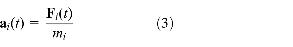
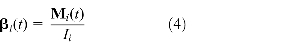
The solid object of study is divided into a set of two-dimensional (2D) rigid circular elements in this work. There are one or more forces between two neighboring element pairs, and the motion of each element is governed by Newton’s second law. For element $i$

m_{i} \frac{d^{2} u_{i}}{{dt}^{2}} = F_{i}

(1)

I_{i} \frac{d ω_{i}}{dt} = M_{i}

(2)

where $m_{i}$ is the mass of element $i$ ; $I_{i}$ is inertia moment of element $i$ ; $u_{i}$ is the displacement of the center of mass of element $i$ ; $ω_{i}$ is the rotational velocity of element $i$ ; and $F_{i}$ and $M_{i}$ present the total external force and centroidal moment, which act on the element $i$ , respectively.

Assume that the displacement $u_{i} (t)$ , velocity $v_{i} (t)$ , acceleration $a_{i} (t)$ , rotational velocity $ω_{i} (t)$ , and rotary acceleration $β_{i} (t)$ of element $i$ in time $t$ are known. The differential equations (1) and (2) can be solved by the explicit finite difference method, and equations (3) and (4) can be obtained

a_{i} (t) = \frac{F_{i} (t)}{m_{i}}

(3)

β_{i} (t) = \frac{M_{i} (t)}{I_{i}}

(4)

at time $t + Δ t$

v_{i} (t + Δ t) = v_{i} (t) + a_{i} (t) Δ t

(5)

ω_{i} (t + Δ t) = ω_{i} (t) + β_{i} (t) Δ t

(6)

u_{i} (t + Δ t) = u_{i} (t) + v_{i} (t + Δ t) Δ t

(7)

\begin{matrix} e_{i} (t + Δ t) = e_{i} (t) + ω_{i} (t + Δ t) \times e_{i} (t) Δ t \\ e_{i} (t + Δ t) = \frac{e_{i} (t + Δ t)}{| e_{i} (t + Δ t) |} \end{matrix}

(8)

where $e_{i}$ is used to record the rotation of the element $i$ . $e_{i}$ , which is bound to the element $i$ , is a unit vector, and $Δ t$ is the time step, which is a basic parameter for difference methods of dynamic problems. Usually, the large $Δ t$ may cause instability of analysis, and the small $Δ t$ causes poor calculation efficiency. In a time step $Δ t$ , the impact wave does not pass on to the next element, so $Δ t$ needs to suit formula (9)

Δ t < \frac{D_{min}}{V}

(9)

where $D_{min}$ is the shortest distance between two elements, and $V$ is the speed of an elastic wave. In terms of the solid particle model in this work, $D_{min}$ is the diameter of the solid disk elements. It is obvious that the time step, $Δ t$ , is dependent on the material and the diameter of elements according to formula (9).

Forces between two neighboring elements

There are one or more forces between two neighboring element pairs as mentioned above. These forces can be classified into many kinds according to different action mechanisms, such as elastic force, elastic-plasticity force, and other field forces. Generally, these forces are the state function of elements, such as the positions or/and the velocities. In terms of solid particle model in this work, the elastic force is assumed as the only mechanical interaction between two contact and connective elements. According to their mechanisms in the DEM, the joint types between two neighboring elements can be classified into two different kinds: contact models and connective models. Contact models are the typical joint type of an assemblage of granular materials. In the contact models, because the deformation compatibility conditions are not restricted, they can be used to expediently solve many complicated dynamics problems, such as nonlinear problems and large deformation problems. In the connective models, because there is no space between elements and the deformation compatibility conditions need be considered, they are used to solve mechanical problems of continuum. Unnecessary errors will be caused if only connect models are used to solve discrete medium mechanic problems or only contact models are used to solve continuity medium mechanic problems.

In this article, collagen fibers are discretized into particle chains (connective models) while chondrocytes and proteoglycans are discretized into free particles (contact models). The simulation of the transition process from continuum to non-continuum, such as the crack process of collagen fibers, can be simplified and efficiently executed by replacing contact models with connective ones.

Forces between connective elements

There is no crack in the collagen fibers in the beginning, and the joint types between elements are connective models. The forces between two action neighboring element pairs can be calculated by the relationship between displacement and forces. The normal force, $F_{n, ij}$ , and tangential force, $F_{s, ij}$ , at time $t$ are illustrated in Figure 1

\begin{matrix} F_{n, ij} (t) = F_{n, ij} (t - Δ t) + k_{n} Δ u_{n} \\ F_{s, ij} (t) = F_{s, ij} (t - Δ t) + k_{s} Δ u_{s} \end{matrix}

(10)

where $Δ u_{n}$ and $Δ u_{s}$ are the increment of relative displacements between element $i$ and $j$ along the normal direction ( $n_{ij}$ ) and the tangential direction ( $s_{ij}$ ), respectively, as shown in Figure 2. $k_{n}$ and $k_{s}$ are spring constants. Notice that the interaction forces between elements $i$ and $j$ are defined as compression/tension and shear.

Figure 1.

Connective model.

Figure 2.

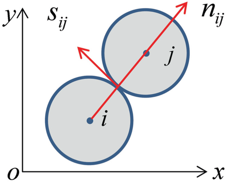
Normal and tangential directions between elements $i$ and $j$ .

Forces between contact elements

After cracks occurred in the collagen fibers, the joint type between the corresponding elements translates from connective to contact. Initially, the neighboring elements in the chondrocytes and proteoglycans are contact models.

Whether two element pairs in 2D are real contact needs to satisfy equation (11).

\sqrt{{(x_{i} + x_{j})}^{2} + {(y_{i} + y_{j})}^{2}} \leq r_{i} + r_{j}

(11)

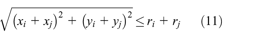
where $i (x_{i}, y_{i})$ and $j (x_{j}, y_{j})$ are the coordinates of the centers of elements $i$ and $j$ , respectively; $r_{i}$ and $r_{j}$ are radii of elements $i$ and $j$ , respectively.

If two elements $i$ and $j$ contact, the normal and tangential forces at time $t$ are illustrated in Figure 3

\begin{matrix} F_{n, ij} (t) = F_{n, ij} (t - Δ t) + k_{jn} Δ u_{n} \\ F_{s, ij} (t) = F_{s, ij} (t - Δ t) + k_{js} Δ u_{s} \end{matrix}

(12)

where $k_{jn}$ and $k_{js}$ are spring constants. Notice that the interaction forces between elements $i$ and $j$ are defined as compression and shear. The shearing contact force is defined along the tangential direction ( $s_{ij}$ ). As shown in Figure 2, if the shearing contact force exceeds the maximum static frictional force, slide contact would occur. The shearing contact force is given as

F_{s, ij} (t) = μ | F_{n, ij} (t) |

(13)

where $μ$ is the slide frictional coefficient between two contact elements.

Figure 3.

Contact model.

Failure criterion of connective models

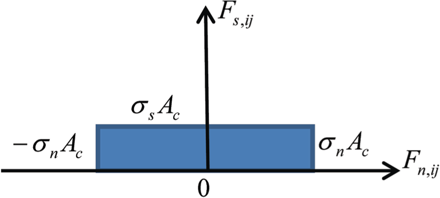
In this work, the failure criterion is shown in Figure 4, where the shaded portions denote the safety zone. If the forces are in the shaded portions, there is no crack occurrence. As shown in Figure 4, the normal force and tangential force are $F_{n, ij}$ and $F_{s, ij}$ , respectively; and $σ_{s}$ and $σ_{n}$ are the tangential and normal strength, respectively.

Figure 4.

Failure criterion of connective models.

The failure criterion of connective models is shown in Figure 4. The interaction forces between connective element pairs are defined as tension, compression, and shear. When tension forces exceed the tensile failure criterion $σ_{n} A_{c}$ , crack occurs. Otherwise, when connective forces are less than the compression limit $- σ_{n} A_{c}$ , compression failure occurs, but the connection does not crack. In the case of shear force, the connective model is adopted for failure criterion, and when $F_{s, ij} > σ_{s} A_{c}$ , shear failure takes place.

Once the tension failure happens, the joint type of inter-element is changed from connect to non-contact. Otherwise, the shear failure happens, and the joint type of inter-element is changed from connect to contact.

Fluid coupling based on particle model

Studies on the fluid–solid coupled particle model are mainly concentrated on two-phase flow.¹⁷ Usually, the solid particle phase which is treated as a pseudo-fluid and fluid phase is solved with the Navier–Stokes Equations. In this method, the whole system is regarded as a mixed fluid. The other method uses the confirmed particle orbital model to describe the solid particle phase and uses the Navier–Stokes Equations to solve the fluid phase. In the above two methods, particle and fluid phases are of large motion. In this work, collagen fibers are discretized into particle chains, whereas chondrocytes and proteoglycans are discretized into free particles. In a dense granular system, solid particles are subjected to the compressions of pore fluid and other particles. Solid particle phase is small motion, and the main motion is that the inner pore fluid flows among the particles. This progress is similar to seepage.

Fluid–solid coupled 2D particle models for different purposes with different approaches have been studied.^18,19 In this work, a fluid–solid coupled particle model is a combination of a discrete particle model and a flow network model. The discrete particle model is described by the DEM. The flow network model is constructed with the pore space in the particle assemblage and will be updated with the deformation and damage developments in the solid particle frame. The impact of the liquid phase on the solid particle frame will also be measured by applying pore pressure on the solid particle elements. The flow of fluid in the pore network is solved with a time-stepping approach. The pore system in the discrete particle model consists of pores connected by pipes. Here, the wide spaces in the pore system are called pores. The throats between the pores are called pipes.

Construction of flow network

In this work, a 2D fluid network model is introduced. The flow network model is constructed in two steps. In the first step, three neighboring particles create a pore enclosed by a triangle (see Figure 5(a)). The pore has three pipes corresponding to the three sides. The pore volume is related to the area enclosed by the three particles. Due to the limit of the 2D model, the flow paths, that is, pipes, are invisible. A virtual flow path is assumed, as illustrated in Figure 6. Assuming there is a third virtual particle element lying out of the 2D model plane and bordering with the two particle elements in the model, the three particle elements form a pipe. It should be noted that such a pipe is unrealistic. In the second step, some of the pores will be merged into pore clusters, which are enclosed by polygons, as shown in Figure 5(b). The condition of pore coalescence is that the pipe conductance is larger than a predefined critical value. Pore coalescence helps to improve the computational efficiency since the number of pores used in the calculation is reduced. Widely open pores are avoided since otherwise they will easily take in fluid. In addition, small time steps should be used in the calculation. However, pore coalescence reduces the accuracy of the calculation. The error is related to the conductance threshold for triggering pore coalescence.

Figure 5.

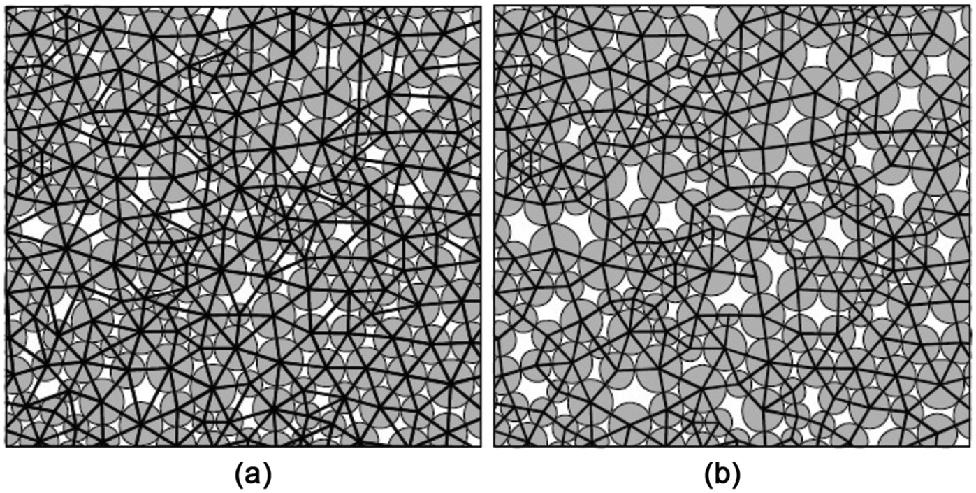
Construction of 2D flow network model: (a) pores first created, enclosed by triangle; (b) after merging, cluster pores enclosed by polygons.

Figure 6.

Flow path. A virtual third particle has to be assumed to calculate the flow path in the 2D model.

Update of flow network

The scheme of constructing the flow network in two steps is not fixed. With the deformation and damage developments in the discrete particle model, updating the flow network in coupling calculation is convenient. If the triangle mesh is limitedly distorted with the deformation of the particle assemblage, the data structure of the pores does not need updating. Only the parameters of the pore system need to be recalculated. However, the pore clusters should be remerged according to recalculated pipe conductance which is changed with the deformation. Only very few additional computational cost is required for this step.

Explicit solution of flow network

Mow et al.⁵ treated the fluid in the articular cartilage as an ideal fluid, which corresponded to the property of the laminar flow. So the micromechanism of the pore flow is assumed to be consistent with Hagen–Poiseuille’s pipe flow. As far as the fluid is concerned, the pipe is equivalent to a round channel. The flow rate in a pipe is given by

q = \frac{{ka}^{3} (p_{2} - p_{1})}{l}

(14)

where $k$ is a conductivity factor; $l$ and $a$ are the length and aperture of a round channel, respectively; and $(p_{2} - p_{1})$ is the pressure difference between the two adjacent pores. The sign convention is such that a positive pressure difference produces a positive flow from pore 2 to pore 1. The length of the pipe is taken to be the sum of the radii of the particle elements which are adjacent to the contact or connection in question.

Each pore receives flows from its surrounding pipes. In one time step, the increase in fluid pressure is given by the following equation, assuming that inflow is taken as positive

Δ p = \frac{K_{f}}{V_{p}} (\sum q Δ t - Δ V_{p})

(15)

where $K_{f}$ is the fluid bulk modulus, $V_{p}$ is the apparent volume of the pore, $\sum q$ are the flow rates from all the surrounding pipes, and $Δ t$ is the time step. The second term in the equation represents the mechanical change in the volume of the pore.

Mechanical coupling

Three forms of coupling between the fluid and the solid particle elements are shown as follows:

The changes of the aperture, which can induce the changes of flow resistance, are caused by contact or connection opening and closing or by changes in the interaction force.

The mechanical changes in the pore volumes cause changes in pressure in the pore.

The pressure in the pores exerts tractions on the enclosing particle elements.

The first two forms of coupling have already been discussed. To simplify the problem of applying pressure forces to particle elements, we assume that the pressure drop due to flow through a pipe is localized at the corresponding contact or connective particle elements. Then, the pressure in the region of the pore is uniform, and the tractions are independent of the path around the pore. If we choose the polygonal path that joins the contacts or connections that surround a pore, the force vector on a typical particle element is

{F'}_{i} = ps n_{i}

(16)

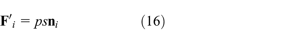
where $n_{i}$ is the unit normal vector of the line joining the two joint points on the particle, and $s$ is the length of the line. As a result, the force vector of particle element $i$ is $F_{i} + {F'}_{i}$ .

Solution scheme

The explicit solution scheme is used for the calculation alternates between applying the pressure equation to all the pores and applying the flow equation to all the pipes. The critical time step for stability is found as follows. Consider a pressure perturbation, $Δ p_{p} = p_{2} - p_{1}$ , in a single pore. The flow into the pore due to the perturbation is then calculated from equation (14) as

q = \frac{{Nka}^{3} Δ p_{p}}{2 R}

(17)

where $N$ is the number of pipes connected to the pore; and $R$ is the mean radius of the particle elements surrounding the pore. According to equation (15) $Δ V_{p} \approx 0$ , this flow causes a pressure response, $Δ p_{r}$ , and it is as follows

Δ p_{r} = \frac{K_{f} q Δ t}{V_{p}}

(18)

For stability, the pressure response must be less than the original pressure perturbation. From equations (17) and (18), the critical time step for stability is satisfied as follows

Δ t = \frac{2 {RV}_{p}}{{NK}_{f} {ka}^{3}}

(19)

As a result, in the fluid coupling based on the particle model, the time step needs to suit formulas (9) and (19).

Numerical simulations

Background of experiment

Considering the difference in the mechanical properties of the surface zone, middle zone, deep zone, and the whole zone in an articular cartilage, we have performed uniaxial compression tests for all three levels of articular cartilages from pigs. The compressive specimens of 120 µm thickness were prepared, cut across the surface, middle, and deep zones using a sledge microtome, and subsequently frozen in saline at −20°C prior to testing, as shown in Figure 7. Both the top and the bottom plates were made using a Petri dish (Figure 7). An aluminum rod was attached between the actuator and the top plate. Both plates and the aluminum rod were covered with a Teflon film. This helped to reduce the transverse friction during testing. A stress–strain curve was generated for all three zones of all specimens. The compressive capacity of articular cartilage is found to increase with the distance measured from the surface. The numerical values of each zone fall into the interval between 50 and 60 MPa, and the numerical value of the whole is about 50 MPa.²⁰ Unfortunately, such a compressive experiment is incapable of obtaining the interior fracture details of the microscopic structure. As a result, the microscopic damage mechanism of articular cartilage cannot be revealed.

Figure 7.

Compressive specimens of 120 µm thickness and compression clamps.

Process of numerical simulations

Alternatively, we resort to explain the damage mechanism of the microscopic structure of articular cartilages by the numerical scheme described above.

The structure of an articular cartilage¹ is illustrated in Figure 8. The collagen fibers are almost parallel to stroma in the surface zone, randomly distributed and form a network structure in the middle zone, and are almost perpendicular to stroma in the deep zone. There are chondrocytes and proteoglycans lying between neighboring zones. The collagen fibers are discretized into particle chains, whereas chondrocytes and proteoglycans are discretized into free particles. Water and electrolyte fill the pores among particles. The detailed structures of the three and whole zones are shown in Figure 9. The red bonded particles denote the collagen fiber particle chains, while the blue free particles denote chondrocytes and proteoglycans. The particles on the bottom layer are fixed, while the middle particles on the top layer are subjected to a uniformly distributed load. The left and right sides satisfy free boundary conditions. In order to avoid the interruption of simulation due to the splash of free particles without confinement, the fixed boundary conditions are applied at 2 diameters of particle elements away from both the left and right sides. In the meantime, the externally distributed loads act within 7 diameters away from both the left and right boundary.

Figure 8.

Cartilage structure.

Figure 9.

Computational model of articular cartilage: (a) surface zone, (b) middle zone, (c) deep zone, and (d) whole zone.

Determining the inner parameters in DEM is a very difficult task. All kinds of theoretical methods predict drastically different values from the real results. In order to deduce the number of computational parameters, the spring constants are used in the connective model and the contact model usually assumes the same value. It is the collagen network that maintains the stability of articular cartilages. In addition, the collagen network calcifies gradually from the surface toward the deep zone. Articular cartilages therefore behave less flexible and more rigid in regions close to the deep zone.¹ As a result, both the normal and tangential stiffness coefficients of a collagen particle element increase with its distance from the surface. The parameters of particle elements are shown in Table 1. The computational parameters of four different zones are shown in Table 2. Simulations for four different zones of articular cartilage under external loads ranging from 40 to 60 MPa are performed.

Table 1.

Parameters of particle elements.

Parameters of particle elements	Proteoglycans and chondrocytes	Collagen in surface zone	Collagen in middle zone	Collagen in deep zone
Density of particle (kg/m³)	1000	2000	2500	3000
Normal spring constants (N/m)	2 × 10⁸	2 × 10⁸	2.1 × 10⁸	2.2 × 10⁸
Tangential spring constants (N/m)	2 × 10⁸	2 × 10⁸	2.1 × 10⁸	2.2 × 10⁸
Friction coefficient	0.1	0.1	0.1	0.1
Normal strength (N/m²)	–	2 × 10⁸	9 × 10⁸	1 × 10⁹
Tangential strength (N/m²)	–	2 × 10⁸	9 × 10⁸	1 × 10⁹

Table 2.

Computational parameters.

Computational parameters	Value
Computational domain (length × height) (µm²)	120 × 300
Radius of particle elements (µm)	Random distribution from 1.5 to 2
Computational time step (µs)	1.439 × 10⁻⁵
Conductivity factor	1 × 10⁻⁹
Fluid bulk modulus (Pa)	2.2 × 10⁹
External load (MPa)	From 40 to 60

Results of numerical simulations

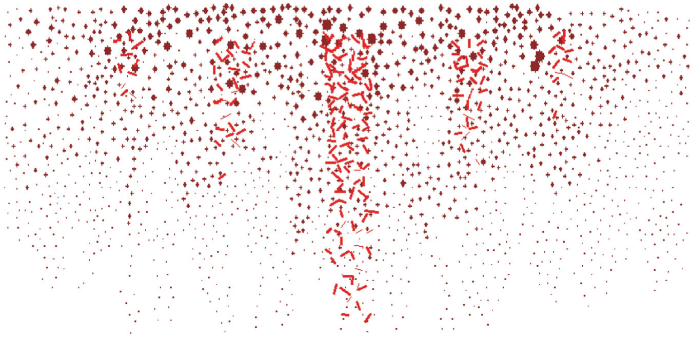
Figure 10 shows a snapshot during the microstructural damage of the surface zone under an external load of 50 MPa. The dots represent the pressure of pore liquid and the red dashes represent the breaking of connective collagen fiber particle elements. It is important to note that the propagation speed of force in liquid is much less than that in solid particles. Therefore, the force between particle elements is large enough to break some bonds of the connective collagen fiber particle elements when the pressure of pore liquid is still low. It is obvious that the microstructural damage of the surface zone is a result of the parallel breakdown of the entire collagen fiber particle elements. That is to say that the surface zone is sliced along the tangential direction. Such a mechanism agrees well with that found in Panula et al.³ and Lewis and Johnson.⁴ In a typical simulation, the failure process of the entire collagen fiber network in the surface zone is as follows. A bond of connective collagen particle elements breaks in the middle of the first layer (Figure 9(a)). This can be regarded as a micro-crack in solid mechanics. With the propagation of the internal forces, more and more micro-cracks are generated in the first layer and results in localized micro-fracture. Micro-cracks start to form in the second layer. The coalescence of micro-fracture forms a parallel cracking zone in the first layer. Micro-fracture is further produced in the second layer and eventually micro-cracks propagate downward.

Figure 10.

A snapshot during the damage process of microstructure in the surface zone of articular cartilage under 50 MPa load.

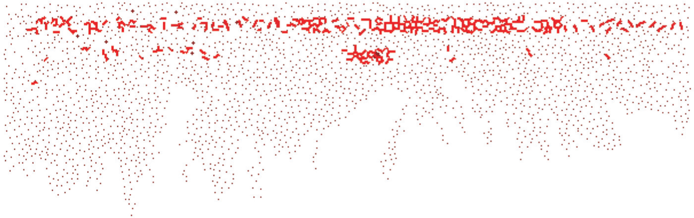
Figure 11 shows another snapshot during the damage process of the microstructure in the deep zone of articular cartilage under 58 MPa load. It is shown that the horizontal breaking of the entire collagen fiber particle elements results in the damage of the microstructure in the deep zone. This means that the deep zone is split along the horizontal direction in the late stage of the injury. During the simulation, the failure process of the entire collagen fiber network in the deep zone is as follows. Micro-cracks first occur on the top in the center level (Figure 9(c)) of the horizontal direction. With the propagation of the internal forces, more and more micro-cracks propagate downward and result in localized micro-fracture on the top in the first set of the horizontal direction. The subsequent downward coalescence of micro-fracture forms a horizontal cracking zone in the center level. Micro-fracture is further produced in the first set, accompanied by the propagation of micro-cracks in the second set.

Figure 11.

A snapshot during the damage process of microstructure in the deep zone of articular cartilage under 58 MPa load.

The simulations of the damage process of the microstructures in different zones of articular cartilage reveal that the injury mechanism of articular cartilage is related to the detailed microstructures of collagen network. The failure of the surface zone is along the tangential direction, while the deep zone splits along the horizontal direction. The middle zone forms a network structure and the exact failure mode depends on the direction of the network. The uncertainty of the network direction makes the injury mechanism of articular cartilages complicated and difficult to predict.

The simulations of three different zones of articular cartilages under external loads ranging from 40 to 60 MPa are performed. It is found that the micro-cracks first appear in the surface zone under 45 MPa. More and more micro-cracks gradually occur as the load increases, and the collagen networks in the surface zone are completely damaged under 53 MPa. Under 48 MPa, the first layer in the surface zone is totally damaged and other layers break locally. Based on this observation, the compressive capacity of the surface zone can be taken as 48 MPa. For the middle zone, micro-cracks first appear under 53 MPa and collagen networks are completely damaged under 58 MPa. Under 56 MPa, the upper layer of the middle zone is totally damaged and localized damage occurs at other layers. The corresponding compressive capacity of the middle zone can therefore be taken as 56 MPa. For the deep zone, micro-cracks first appear under 55 MPa and collagen networks are completely damaged under 60 MPa. Under 57 MPa, the center layer in the middle zone is totally damaged and the first set breaks locally. As a result, the compressive capacity of the middle zone can be taken as 57 MPa. The relationship between the damage of articular cartilage and external loads is tabulated in Table 3.

Table 3.

The relationships between the damage of articular cartilage and external load.

Positions of articular cartilage	Load of initial micro-cracks (MPa)	Load of complete damage (MPa)	Load of compressive capacity (MPa)
Surface zone	45	53	48
Middle zone	53	58	56
Deep zone	55	60	57

As shown in Table 3, the compressive capacity of articular cartilages increases with the distance measured from the top surface. The numerical interval (48–57 MPa) agrees well with its experimental counterpart (50–60 MPa of each zone) as shown in Mageswaran.²⁰

Figure 12 shows another snapshot during the microstructural damage of the whole articular cartilage subjected to a 49-MPa load. It is shown that the first layer fibrous network of the surface zone is entirely broken. However, with the propagation of the internal forces, the fibrous network of the middle and deep zones is not broken. It is further found that the micro-cracks first appear in the whole zone when the external load reaches 46 MPa. The surface zone became tangentially sliced under slightly elevated pressure (49 MPa), suggesting that the articular cartilage as a whole system has lost its functionality. This pressure magnitude agrees very well with the experimental value of the whole zone, that is, roughly 50 MPa in Mageswaran.²⁰

Figure 12.

A snapshot during the microstructural damage of the whole articular cartilage subjected to a 49-MPa load.

Conclusion

Given the fact that both experiments and FEM are unable to reveal the injury mechanism of articular cartilages, we have proposed a new numerical method based on the fluid–solid coupled discrete particle model. The process from the damage of collagen network to the injury of articular cartilage under external loads is investigated in detail for revealing the microscopic damage mechanism of articular cartilages. A variety of numerical simulations were performed to validate the accuracy and robustness of the developed method.

The injury mechanism of an articular cartilage is related to the microstructure of its collagen network. The failure of the surface zone is along the tangential direction, while the deep zone splits along the horizontal direction. The middle zone forms a network structure and the exact failure mode depends on the direction of the network. The uncertainty of the network direction makes the injury mechanism of articular cartilages complicated and difficult to predict.

The compressive capacity of an articular cartilage increases with the distance measured from its top surface. It is 48 MPa for the surface zone and increases to 56 and 57 MPa for the middle and deep zones, respectively.

The surface zone became tangentially sliced under the pressure level of 49 MPa. Although the middle and deep zones remain unbroken, the tangential slicing of the surface zone suggests that the articular cartilage as a whole has lost its functionality.

Footnotes

Academic Editor: Chuanzeng Zhang

Declaration of conflicting interests

The authors declare that there is no conflict of interest.

Funding

This work was supported by the National Natural Science Foundation of China (Grant Nos 11302049, 11202051) and the Scientific Research Foundation for the Returned Overseas Chinese Scholars, State Education Ministry.

References

Mow

. Basic orthopaedic biomechanics. Philadelphia, PA: Lippincott-Raven, 1997.

Bank

Soundry

Maroudas

. The increased swelling and instantaneous deformation of osteoarthritic cartilage is highly correlated with collagen degradation. Arthritis Rheum 2000; 43: 2202–2210.

Panula

Hyttinen

Arokoski

. Articular cartilage superficial zone collagen birefringence reduced and cartilage thickness increased before surface fibrillation in experimental osteoarthritis. Ann Rheum Dis 1998; 57: 237–245.

Lewis

Johnson

. Collagen architecture and failure processes in bovine patellar cartilage. J Anat 2000; 199: 483–492.

Mow

Kuei

Lai

. Biphasic creep and stress relaxation of articular cartilage in compression: theory and experiments. J Biomech Eng Trans ASME 1980; 102: 73–84.

Lai

Mow

Roth

. Effects of nonlinear strain-dependent permeability and rate of compression on the stress behavior of articular cartilage. J Biomech Eng Trans ASME 1981; 103: 61–66.

Soulhat

Buschmann

. Nonlinear analysis of cartilage in uncontained ramp compression using a fibril reinforced poroelastic model. Clin Biomech 1999; 14: 673–682.

Chegini

Ferguson

. Time and depth dependent Poisson’s ratio of cartilage explained by an inhomogeneous orthotropic fiber embedded biphasic model. J Biomech 2010; 43: 1660–1666.

Hai-yu

Yuan-chao

Cheng-tao

. Articular cartilage simulation using depth-dependent mechanical parameters. J Med Biomech 2011; 26: 168–172.

10.

Wen-jie

Zhong-yong

. Finite element analysis on unconfined compression of cartilage tissues. J Med Biomech 2012; 27: 630–635.

11.

Li-lan

Chun-qiu

Zhi-dong

. Normal displacement of different layers for articular cartilage under sliding loads. J Med Biomech 2014; 29: 21–24.

12.

Potyondy

Cundall

. A bonded-particle model for rock. Int J Rock Mech Min Sci 2004; 41: 1329–1364.

13.

Oda

Yasuda

. On impact penetration analysis and evaluation of brittle material plate using three-dimensional DEM. Trans Jpn Soc Mech Eng 2005; 71A: 1554–1559.

14.

Kim

Buttlar

. Discrete fracture modeling of asphalt concrete. Int J Solids Struct 2009; 46: 2593–2604.

15.

Zang

Lei

Wang

. Investigation of impact fracture behavior of automobile laminated glass by 3D discrete element method. Comput Mech 2007; 41: 73–83.

16.

Qi-cheng

Guang-qian

. Mechanical introduction of granular materials. Beijing, China: Science Press, 2009.

17.

Jing-hai

. Multiscale simulation of granular and fluid complex system. Beijing, China: Science Press, 2005.

18.

Itasca Consulting Group. Verification problems and example applications. Minneapolis, MN: Itasca Consulting Group, 2005.

19.

Bruno

Dorfmann

Lao

. Coupled particle and fluid flow modeling of fracture and slurry injection in weakly consolidated granular media. In: Proceedings of the 38th US rock mechanics symposium, Washington, DC, 7–10 July 2001, pp.173–180. Alexandria, VA: American Rock Mechanics Association.

20.

Mageswaran

. Experimental determination of the non-linear, large strain zonal mechanical properties of cartilage for use in quasi-static finite element model. North Carolina State University, Raleigh, NC, 2005, http://repository.lib.ncsu.edu/ir/bitstream/1840.16/1130/1/etd.pdf

Study on the damage mechanism of articular cartilage based on the fluid–solid coupled particle model