Sage Journals: Discover world-class research

Abstract

In order to improve the acoustic attenuation performance of an exhaust muffler of a 175 series of agricultural diesel engine, automatic matched layer method of finite element is adopted on the basis of LMS Virtual.Lab software to simulate the non-reflecting boundary conditions, which can avoid the complex calculation and then figure out the value of propagated sound power directly and finally obtain the transmission loss of the exhaust muffler. Compared with the experimental data, it can be found that the error between the simulation and measured values is small, and it can be accurately simulated for the acoustic performance of the exhaust muffler at the frequencies smaller than 3000 Hz, which verifies the validity of the acoustic solution. An improved design that properly distributes the insertion length of intubation, increases the length–diameter ratio, and adds the length of the first expansion cavity is proposed for the poor acoustic attenuation performance in low and medium frequencies. Compared with the original design, the transmission loss value at low and medium frequencies obviously increases, so the acoustic attenuation performance at the frequencies becomes better.

Keywords

Diesel engine exhaust muffler transmission loss acoustic simulation

Introduction

Along with the rising motor vehicle population, the noise pollution becomes serious and exhaust noise has become the main noise source of an engine, so the acoustic attenuation performance of an exhaust muffler which has been adopted as the most effective method in dealing with exhaust noise seems particularly important.^1,2 At present, the main research methods for measuring the acoustic performance of the exhaust muffler include transfer matrix method, finite element method, and boundary element method,³ while the finite element method has become the commonly used three-dimensional analysis method because of its good adaptability.⁴ Finite element method can simulate various types of mufflers, especially suitable for solving the muffler that has complex shape and cross-sectional structure; meanwhile, the acoustic precision is higher at low and medium frequencies.^5–7 Since Clough et al. proposed the finite element technology that had achieved rapid development in the engineering field for the first time, many experts, both domestic and abroad, have been doing research on it intensively. Craggs⁸ first attempted to analyze the muffling characteristics of noise elimination unit based on the finite element method which laid a consolidating foundation for the finite element method applied in the field of acoustic. Young and Crocker^9,10 adopted the finite element two-dimensional analysis method in the calculation of the muffler’s transmission loss (TL) for the first time, which promoted the further study of finite element method applied in the muffler. Ross¹¹ used finite element method to analyze the muffler’s muffling characteristics which contained perforated structure. Mechel¹² described the finite element method applied in the different structural muffler’s acoustics research in his monograph. Rong and Zhengshi¹³and Jing¹⁴ utilized the acoustic finite element method, took complex muffler as the research object, and focused on its acoustic characteristics analysis method. Guanxin¹⁵ explored the way of combining the use of transfer matrix method and finite element method and provided reliable theoretical method for the muffler’s optimization design. Qihui¹⁶ considered the air temperature as an influencing factor and used the finite element method to calculate the practical muffler’s TL. Lei¹⁷ calculated different types of perforated pipe muffler’s TL based on the finite element method as well as studied various factors affecting the acoustic performance of perforated pipe frame of the muffler.

In this article, in order to improve the acoustic attenuation performance of the exhaust muffler of a 175 series of agricultural diesel engine, automatic matched layer (AML) method of finite element is adopted on the basis of LMS Virtual.Lab software to simulate the non-reflecting boundary conditions, which can avoid the complex calculation and then figure out the value of propagated sound power directly and finally obtain the TL of the exhaust muffler. Compared with the experimental data, it will be found whether the simulation model verifies the validity of the acoustic performance at the frequencies from 1 to 3000 Hz. Finally, the improved scheme will be put forward, and based on the above verified model, it will be found out whether the acoustic attenuation performance of the muffler is better by simulation.

Muffler modeling

Geometric parameters

As shown in Figure 1, the exhaust muffler has two resonant cavities, namely, first resonant cavity V₁ and second resonant cavity V₂, while the total length L and the diameter D are 140 and 82 mm, respectively; the first resonant cavity length and the second resonant cavity length are 102 and 36 mm, respectively; the inlet intubation length and the exhaust intubation length are 80 and 35 mm, respectively; the specific size is as shown in Table 1.

Figure 1.

2D schematic of an exhaust muffler: (a) external structure figure and (b) internal structure dimension figure.

Table 1.

Structural size of the muffler.

Structure parameters	L	L₁	L₂	L_i	L_o	D	D₁	D₂	D₃	D₄	δ₁	δ₂
Size (mm)	140	102	36	80	35	82	28	23	10	10	1	1

Three-dimensional modeling

As shown in Figure 2, the muffler’s three-dimensional model is established based on UG Software. In addition, Figure 1(a) is the shell model that is simplified duly by ignoring the influence of attachment screw and fillet, while Figure 1(b) is the acoustic simulation model which has been established via reverse modeling, that is, regarding the internal air flow area in the muffler as a discrete entity and dispersing it, just like removing the shell and obtaining internal simulation entities.

Figure 2.

3D schematic of an exhaust muffler: (a) shell diagram and (b) flow diagram.

Mesh generation

The geometry of the muffler is relatively complex, and there are more perforation and interpolation tubes that are not suitable for adopting to divide the hexahedron structured grid for all. However, for the simple tetrahedral mesh, too large size will easily cause calculation error at the perforation region and too small one will decrease the amount of calculation.¹⁸ As for this article, the method of dividing a region to certain blocks is adopted to mesh with mixed grid shapes. First, as shown in Figure 3(a), each structure is defined corresponding to different colors; besides, 2.0 mm tetrahedral mesh is used for the intake and exhaust pipes, 0.5 mm tetrahedral mesh is used for each perforation, and 3 mm hexahedron structured mesh is used for the central regions with regular shape. Second, the grid cell meshing is shown in Figure 3(b). As for the perforation pipe, due to the adaptive capability of unstructured grids, it can match with structured grids, which ensured the integrity of grids. As shown in Figure 3(c), the mesh size is able to cover up the whole circular cross section, simulate the small holes more realistically, and guarantee the calculation accuracy; besides, the feature of simple data structure of the hexahedron structured grid at the central regions with regular shape can effectively decrease the number of grid and the amount of calculation as far as possible. Finally, the total numbers of grids cells and nodes are 1,015,602 and 180,044, respectively, while the total number at small hole is 345,664.

Figure 3.

Mesh generation diagram: (a) definition of each part, (b) whole grid, and (c) small hole grid.

As the LMS acoustic analysis needs high-quality grid, the mesh quality generated by LMS is rough. Therefore, in order to verify the integrated computer engineering and manufacturing (ICEM) mesh quality, ICEM grid is compared with LMS grid. Figure 4 shows the comparison of acoustic mesh. Figure 4(a) shows that both the ICEM external mesh and LMS external mesh are well distributed and there is no much difference. However, as for the LMS generating grid as shown in Figure 4(b), its inner grids have no regular growth law and larger size deviation. To the contrary, as for the ICEM generating grid shown in Figure 4(c), its inner grids distribute well; meanwhile, both the grid size and growth law are better. Thus, it verifies that the meshing method is feasible and will reduce the influence of the grid quality on acoustic simulation calculation.

Figure 4.

Comparison of acoustic mesh: (a) external grid, (b) LMS generating grid, and (c) ICEM generating grid.

Muffler acoustic simulation

Boundary conditions definition

First, the fluid material among the muffler is defined as air, whose velocity is 340 m s⁻¹ and density is 1.225 kg m⁻³. Then, the upper computation frequency limit is checked after setting the properties of the fluid material, and it is found that the computation frequency of grid cells is up to 4000 Hz which can ensure the calculation accuracy at the frequencies. Second, the inlet acoustic boundary conditions are defined as the one-order plane wave with 1 W sound power. Later, as the form of acoustic transfer at the inlet and outlet ends of a vehicle muffler is basic plane wave, the AML can be used to define the outlet boundary conditions as non-reflecting boundary conditions directly. Finally, the wall boundary conditions are defined as rigid plane by neglecting the wall’s sound absorption.

Frequency characteristic analysis

The acoustic pressure contours whose frequencies are 250, 1000, 1500, 2000, 2500, and 3000 Hz, respectively, are depicted in Figure 5. It shows that acoustic pressure contours of the muffler accord with one-dimensional plane wave theory and the sound transfers mainly in the form of plane wave at low and medium frequencies from 250 to 1000 Hz. After further analysis of the contour at 250 Hz, it is found that the acoustic pressure presents a trend of ladder-like distribution, and its amplitude is almost equal on the same cross section. In addition, the contour at 1000 Hz shows that the acoustic pressure distribution reflects the transfer law of plane wave, yet although part of it appears as a small-scale fluctuation. Then, when frequency is between 1000 and 2000 Hz, the contour shows that the acoustic pressure distributes irregularly; in addition, the acoustic pressure amplitude at 1500 Hz begins to appear as large fluctuation. Finally, when the frequency is increased to 2500–3000 Hz, the acoustic pressure distributes unevenly and appears as a significant circumferential and radial fluctuation. To sum up the above arguments, it is concluded that the sound during the process of transmission will produce higher harmonic with the increase in frequency; meanwhile, acoustic pressure distribution is uneven and the amplitude varies significantly, which lead to inapplicability of the theory on the plane wave; however, the three-dimensional acoustic theory can simulate the internal sound field at high frequency exactly.

Figure 5.

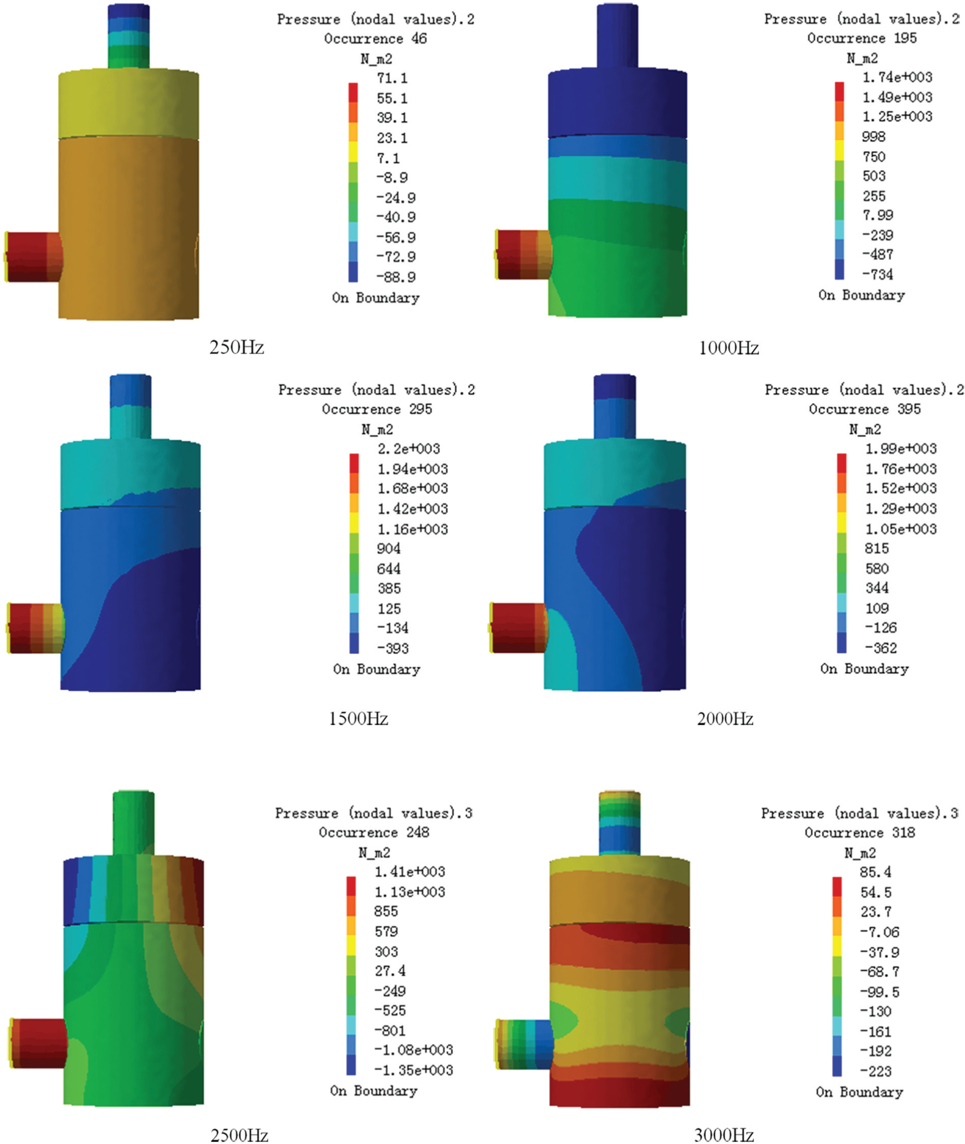
Frequency acoustic pressure contours.

TL calculation

TL is the difference between incident sound power level at the inlet and transmission sound power level at the outlet. The traditional calculation equation of TL is described as equation (1)

TL = 10 \log (\frac{W_{in}}{W_{out}}) = 10 \log (\frac{p_{in} {\bar{p}}_{in}}{p_{out} {\bar{p}}_{out}} \frac{A_{in}}{A_{out}})

(1)

where W_in and W_out are the sound power of inlet and outlet plane waves, respectively; p_in and p_out are the inlet and outlet acoustic pressures, respectively; A_in and A_out are the area of inlet and outlet cross sections, respectively.

During the process of acoustic computation, the acoustic pressure p is a plural, which leads to the calculation of equation (1) being complicated and also needs to consider the area of inlet and outlet sections. However, the AML method can avoid complicated calculation and being unaffected by the area of inlet and outlet sections; besides, it can directly define a certain sound power value as the boundary conditions at the inlet. Accordingly, TL of the muffler can be calculated by equation (2) as follows

TL = 10 \log \frac{Wi}{Wt}

(2)

where W_i and W_t are the sound power of inlet and outlet plane waves, respectively.^19–21

From the TL graph, as shown in Figure 6, it can be found that TL at high frequencies of over 3000 Hz produces many resonance peaks. There are a lot of passing frequencies, and the variation difference of acoustic pressure between the frequencies becomes large, which is as a result of the existing cut-off frequency of the muffler, and above it there are many failure frequencies which have little practical reference value. Thus, the TL at frequencies between 1 and 3000 Hz is mainly analyzed as follows. First, the average TL is 10 dB at low frequencies from 1 to 1000 Hz; as a result, the effect of acoustic attenuation is non-ideal. Second, the average TL can be up to 45 dB at middle and high frequencies from 1000 to 3000 Hz and it produces resonance peaks at frequencies of 2200, 2700, and 3005 Hz while the average TL is larger than 50 dB, especially at the frequency of 2200 Hz up to 60 dB which has the best effect of acoustic attenuation. Finally, for the TL of the muffler, there exist two passing frequencies, which are 24 and 1100 Hz, where there is almost no effect of acoustic attenuation at frequencies from 1 to 3000 Hz; besides, the TL has low value at 2000 and 3000 Hz where the effect of acoustic attenuation is poor.

Figure 6.

Graph of muffler transmission loss.

Muffler exhaust noise test

Test equipments

TL (sound power level difference) and insertion loss (IL) (acoustic pressure level difference) are the most important indexes which reflect the acoustic performance of the exhaust muffler from different aspects. At the same time, sound power level and sound pressure level have the following conversion formula¹³

TL = IL + 10 \log (4 π r^{2})

(3)

where r is the distance from sound source to the test points, IL is the insertion loss, and TL is the transmission loss.

Equation (3) shows that when the distance between sound source and test point is a constant value, the difference between TL and IL is only a constant. Because the TL measurement needs special equipments and IL is relatively easy to measure and has good practical effect, in this article, we prioritize using the method of IL measurement.

Consequently, in this article the method of IL measurement is adopted. First, the IL measurement of muffler test bench is set up. Then, the original spectrum of exhaust noise is measured and analyzed, and the accuracy of the simulation model is verified by comparing with acoustic simulation results. Finally, as shown in Figure 7, the test bench setup mainly includes diesel engine, an eddy current dynamometer, an FC2000 diesel engine controlling system, a sound level meter, a spectrum analyzer, and a specially made acoustic board.

Figure 7.

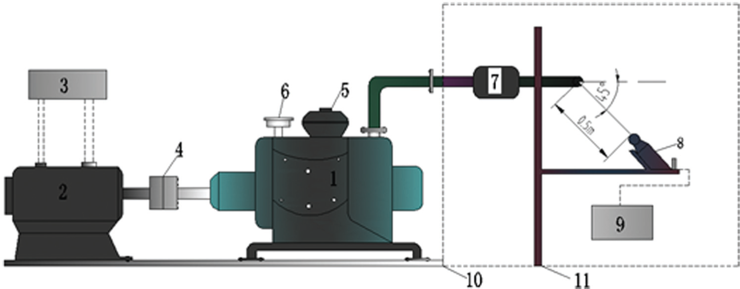
Schematic of test bench.

Measurement of muffler IL

The IL measurement is referred to the national standard GB/T4759-2009 of Internal Combustion Engine Exhaust Muffler Measurement Method strictly.²² First, the diesel engine is started and is kept running stably for a period of time till the temperature of the fuel and cooling water is up to the appropriate value, and then the data are recorded. Second, the noise of not installing an exhaust muffler is measured where an empty tube with equal length and diameter instead of the muffler is used. Meanwhile, the axial position of the measuring point with exhaust port flow ought to be ensured as 45° and the distance 0.5 m. Finally, a special sound insulation board is used to ensure measurement point from the effects of other noises nearby, and the relative position of measurement point and exhaust port should always be kept the same.²³

From the acoustic analysis above, it is concluded that the acoustic attenuation frequencies with the best effect of the reactive muffler are between 31.5 and 3000 Hz, which has good reference value. So this test mainly acquires the signal at the frequencies between 31.5 and 3000 Hz; meanwhile, the sound level at the central frequency is recorded; when the engine is operated under full load, the speed ranges from 1400 to 2600 r min⁻¹ and increases progressively with 200 r min⁻¹. First, the environment background noise is measured and then the acoustic pressure and spectrum with empty tube and muffler installed, respectively, are measured; meanwhile, the related data are gathered and recorded. Second, after collecting the data every time, the engine will be stopped to collect data till the diesel engine runs steadily, and each group of data need to be measured twice. If the measurement difference is greater than 2 dB, it should increase the reading twice, and each result should be recorded. Finally, the poor values may be judged and eliminated with the Pauta criterion;^24,25 as a result, reliability of the experimental data will be ensured.

Simulation and experiment comparative analysis

With the influence of the test environment considered and the test data modified, an A-weighted acoustic pressure measuring chart is drawn, as shown in Figure 8. Then, the acoustic pressure level data at speeds 1400 and 2600 r min⁻¹ before and after installing the muffler are selected for analysis, where the acoustic pressure level values are 101.0 and 85.0 dB, respectively, at the speed of 1400 r min⁻¹ and the IL is calculated as 15.2 dB, while the acoustic pressure level values are 105.6 and 90.3 dB, respectively, at the speed of 2600 r/min and the IL is 15.3 dB. In addition, after analyzing the data at other speeds, it shows that the IL of the muffler is about 15.0 dB. Finally, the average of IL is equal to 15.49 dB; therefore, the amount of acoustic attenuation of the muffler is 15.5 dB.

Figure 8.

A-weighted acoustic pressure measuring chart at all rotation speeds.

The comparison figures of measuring IL with simulation TL at different engine speeds are drawn, as shown in Figure 9, where Figure 9(a) and (b) depicts the actual IL and the simulation of TL, respectively. Based on the previous analysis, the acoustic simulation results of the muffler at frequencies between 31.5 and 3000 Hz have good reference value, and hence the simulation data of transfer TL are exported. From the experiment data, IL is 15.5 dB and based on equation (3), TL is figured out and is equal to 20.45 dB; however, the average TL is calculated as 18.72 dB, and the difference to the actual value is 1.73 dB. This error may be as a result of the muffler being influenced by factors of materials and manufacturing equipments in the machining process. As a whole, the error between the simulation and actual value is not big; accordingly, it is indicated that the acoustic simulation design is feasible.

Figure 9.

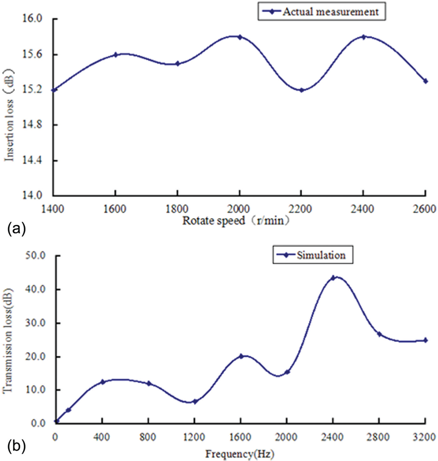
Comparison of measuring insertion loss with simulation transmission loss: (a) actual insertion loss and (b) simulation of transmission loss.

As shown in Figure 10, it is found that most simulation values are lower than the measured ones at the frequencies between 31.5 and 1250 Hz; only at 630 and 800 Hz, the simulation values are higher than the measured. It is as a result of the existence of flow regeneration noise making the calculation model unable to carry on the simulation analysis. After further analysis of the spectrum graph, it is found that at low and medium frequencies, the simulation and measured values fit well; however, at high frequencies the acoustic pressure values have a large difference, especially at frequencies of over 3000 Hz where the error becomes larger and larger. It may be as a result of the emergence of higher harmonic at high frequencies, leading to a reduction in the effect of acoustic attenuation of the muffler and even having no effect of acoustic attenuation. At the same time, the grid quality and the machining error can also cause the error between the simulation and actual values at high frequencies.

Figure 10.

Comparison of the experiment’s and the simulation’s transmission loss at central frequencies.

To sum up the above arguments, it is concluded that the muffler solution model is able to simulate acoustic pressure at the acoustic attenuation frequencies accurately, especially at low and medium frequencies; it fits well, but there is a certain error at high frequencies above 3000 Hz.

Modification analysis

Because the exhaust noise of a 175 series of agricultural diesel engine is mainly focused at low frequencies and is based on the previous analysis, it is concluded that the effect of acoustic attenuation of the muffler at low and medium frequencies is not ideal, especially at frequencies between 20 and 45 Hz as well as between 1000 and 1150 Hz; therefore, it is necessary to adopt measures to improve the effect of acoustic attenuation at low frequencies. At the same time, the expanding cavity V is mainly used to eliminate low and medium frequency noise, and the length of the perforated tubes L_i and L_o has influence on noise absorption at low frequencies; therefore, it will serve as the focus of improvement. First, the length of the expansion cavities L₁ and L₂ being designed unequal to each other can make the passing frequency of each cavity staggered; meanwhile, increasing the length–diameter (L/D) ratio of the cavity properly and designing a more slender muffler will improve the effect of acoustic attenuation at low frequencies considerably. Second, the perforated tube also has a good effect of acoustic attenuation at high frequencies, and the insertion length being designed as the combination of L/2 and L/4 can reduce the influence of passing frequency and improve the effect of acoustic attenuation at low frequencies. Strict adherence to the engine-specific parameter requirements, in view of the structure factors of the retrofit muffler, is put forward. The insertion lengths of the intake and exhaust pipes are attempted to be designed as L/4 and L/2, respectively. In order to improve the muffler, the length of the first expansion cavity V₁ is increased and the L/D ratio is added properly. Scheme I is the original muffler, scheme II is the improved muffler, and specific sizes are shown in Table 2.

Table 2.

Retrofitted size of muffler.

Scheme	L_o (mm)	L_i (mm)	L₁ (mm)	L/D
Original muffler	35	80	102	1.71
Retrofit muffler	42	85	130	2.40

Then, the TL is calculated, and the comparison curves of the TL for the original with the improvement scheme are drawn, as shown in Figure 11, where the blue curve represents the original scheme while the red one represents the improved scheme. As a whole, the TL values at low and medium frequencies between 1 and 2000 Hz increase obviously and the effects of the key improvement frequencies between 10 and 45 Hz as well as between 1000 and 1150 Hz are good. Furthermore, compared with the original scheme, the TL value increases about 12 dB on average; only at high frequencies between 2200 and 2800 Hz it reduces, and at other frequencies it nearly increases; as a result, the effect of acoustic attenuation improves significantly. In the end, the acoustics performance of the muffler has been improved significantly after modification.

Figure 11.

Comparison of pre- and post-transmission loss.

Conclusion

This article is based on LMS Virtual.Lab Software and AML method; after defining the non-reflecting boundary condition, the TL of exhaust muffler which is not much different from the measured values is calculated as around 3.18 dB. By combining with the acoustic pressure comparison contours at the central frequencies, a conclusion can be drawn that the muffler solution model is able to accurately simulate the acoustic pressure at the frequencies between 31.5 and 3000 Hz, which further verify the reliability of the solution method.

Based on this acoustic simulation method, the simulation values of the acoustic pressure among the muffler at low and medium frequencies match with the measured ones well; meanwhile, the difference between the simulation and measured values at high frequencies is large, especially when the frequency is above 3000 Hz.

It is found that the acoustic attenuation effect at low and medium frequencies is poor via analysis of the TL curve. An improvement design that reasonably distributes the insertion length of the perforated pipe, increases the L/D ratio, and adds the length of the first expansion cavity is proposed for the poor acoustic attenuation performance at low and medium frequencies. Compared to the original design, the TL value at low and medium frequencies of the design clearly increases, so the acoustic attenuation performance at the frequencies can be improved.

The structure factor influence on the muffler's acoustic properties needs to be further researched.

Footnotes

Academic Editor: Hongwei Wu

Declaration of conflicting interests

The authors declare that there is no conflict of interest.

Funding

This work was financially supported by the Innovation Platform Open Foundation in Higher Educational Institutions of Hunan Province (No. 12K130), the Aid Program for Science and Technology Innovative Research Team in Higher Educational Institutions of Hunan Province, and the Postgraduate Innovative Research Project of Shaoyang University (No. CX2013SY021).

References

Jin

Guohua

Weiping

. Simulating acoustics performance of exhaust noise of single cylinder diesel engine. Chin Intern Combust Engine Eng 2006; 27: 226–230 (in Chinese).

Riyao

. Noise analysis of diesel generator set and acoustic simulation of exhaust muffler. Guangzhou, China: Guangdong University of Technology, 2013.

Gen

Jiangbo

Haihua

. The research status and trend at home and abroad of acoustic performance on automotive exhaust muffler. Mod Manuf Eng 2012; 12: 127–132 (in Chinese).

Zhongxu

Sifa

Xiaoming

. A study on the numerical simulation method for the acoustic performance of exhaust catalytic muffler. Automot Eng 2011; 33: 226–230 (in Chinese).

Jianguo

Tao

Yushan

. Numerical analysis and structure improvement of automotive exhaust muffler’s acoustic characteristics. Noise Vib Control 2011; 2: 59–62 (in Chinese).

Meiling

. Acoustic characteristic simulation and study of exhaust muffler based on CFD. Jinan, China: Shandong University, 2013.

. The numerical simulation analysis on the exhaust muffler. Dalian, China: Dalian University of Technology, 2013.

Craggs

. An acoustic finite element approach for studying boundary flexibility and sound transmission between irregular enclosure. J Sound Vib 1973; 30: 343–357.

Young

CIJ

Crocker

. Acoustic analysis testing and design of flow-reversing muffler chambers. J Acoust Soc Am 1976; 60: 1111–1118.

10.

Young

CIJ

Crocker

. Finite element acoustical analysis of complex muffler systems with and without wall vibration. Noise Control Eng 1977; 9: 86–93.

11.

Ross

. A finite element analysis of perforated compartment acoustic systems. J Sound Vib 1981; 79: 133–143.

12.

Mechel

. Formulas of acoustics. 2nd ed.Berlin: Springer Verlag, 2008.

13.

Rong

Zhengshi

Yimin

. A study on the acoustic performances of multi-inlet/multi-outlet reactive muffler. Automot Eng 2014; 36: 242–248.

14.

Jing

. Simulation of acoustic and fluid dynamic performance of reactive exhaust mufflers. Chongqing, China: Chongqing University, 2012.

15.

Guanxin

. Study on design method of wide band large noise elimination quantity exhaust muffler. Chongqing, China: Chongqing Southwest Jiaotong University, 2011.

16.

Qihui

. Simulation research on performance of exhaust muffler of automotive based on virtual lab. Chongqing, China: Chongqing Jiaotong University, 2013.

17.

Lei

. Numerical simulation of acoustic characteristic of muffler with perforated pipe. Jinan, China: Shandong University, 2012.

18.

Xiaodong

. Study on resistance muffler based on CFD simulation and test. Jinan, China: Shandong University, 2007.

19.

Fuliang

. Virtual lab acoustics acoustic simulation from introduction to master. Xi’an, China: Northwest Industrial University Press, 2013.

20.

Yan

. Acoustic characteristics simulation of engine exhaust muffler based on CFD. J Vib Eng 2011; 24: 205–209 (in Chinese).

21.

Galland

. Acoustic transmission performance of double-wall active sound packages in a tube: numerical/experimental validations. Appl Acoust 2012; 73: 323–337.

22.

GB/T4759. Internal combustion engine exhaust muffler measurement method. Beijing, China: China Standards Press, 2009.

23.

Yasuda

. Predictions and experimental studies of the tail pipe noise of an automotive muffler using a one dimensional CFD model. Appl Acoust 2010; 71: 701–707.

24.

Jun

Jinke

Wenhua

. Establishment and application of MAP for regeneration back-pressure threshold value of diesel particulate filter. Trans Chin Soc Agric Eng 2013; 29: 47–56 (in Chinese).

25.

Jun