Sage Journals: Discover world-class research

Abstract

This study presents an innovative method utilizing weightless neural networks (WNNs) to identify and address various types of faults in air compressor modules. Random access memory (RAM) devices are harnessed by WNNs to emulate the functioning of neurons. The training process employs a versatile and effective algorithm aimed at generating reliable and accurate results. One notable benefit of employing WNNs is its ability to eliminate the necessity for network retraining and the generation of residuals. This feature makes WNN suitable for applications related to classification and pattern recognition. In this study, a specific type of air compressor, namely a single-acting single-stage reciprocating one, was chosen. Various potential faults like fluttering inlet and outlet valves, valve plate leakage, and check valve issues were taken into account. From the initial vibration data, statistical, histogram, and autoregressive moving average features were derived. For efficiency, the J48 decision tree algorithm was utilized to identify the pivotal features in this investigation. Following this, the features were divided into separate sets to evaluate the validation, training, and testing accuracies of the WNNs using the WiSARD classifier. Additionally, fine-tuning of hyperparameters was done to enhance classification accuracy while simultaneously reducing computational time. The results obtained demonstrate that, with the specified hyperparameter configurations, the WiSARD classifier attained an accuracy of 98.6667% for statistical features. The proposed method outperforms existing approaches, showing potential for real-time application in enhancing air compressor lifespan, reliability, and safety.

Keywords

air compressor fault detection WiSARD machine learning J48 hyperparameter

Introduction

Air compressors are indispensable mechanical devices that convert power (often from electric motors or internal combustion engines) into compressed air stored in tanks. This pressurized air serves as a versatile energy source for a myriad of applications powering everything from pneumatic tools to manufacturing machinery. Their critical role in various industries underscores their significance. When functioning correctly, air compressors ensure the smooth and efficient operation of essential equipment. However, when these crucial components experience faults or malfunctions, they can disrupt machinery and industrial processes, leading to reduced productivity, increased downtime, and potential safety risks. Fault diagnosis, therefore, becomes imperative as it allows for the early detection and identification of issues within air compressors. Timely diagnosis and subsequent maintenance or repairs can prevent catastrophic failures, optimize machinery performance, minimize downtime, and ultimately save both time and resources. In essence, fault diagnosis is a proactive strategy to ensure the reliability and longevity of machinery in industries reliant on compressed air systems.

Within the domain of mechanical systems, the evaluation of signals holds a central position in appraising the well-being and operational status of a variety of elements. There exists a diverse array of signal types and corresponding analytical techniques tailored to specific applications. Selecting the appropriate type of analysis for fault diagnosis is paramount, as each method possesses distinct capabilities and sensitivities. A mismatched choice can lead to missed or misinterpreted indicators of impending issues, potentially compromising the reliability and safety of the mechanical system. Therefore, meticulous consideration of the specific features and operational context of the component in question is essential to ensure accurate and reliable fault diagnosis. The most commonly adopted fault diagnosis techniques for mechanical components are listed as follows¹:

Analysis of Current, Voltage, and Electromagnetic Fields: This approach utilizes electromagnetic monitoring to identify imperfections such as cracks, weaknesses, dents, and corrosion in components. It employs eddy current testing for fault identification that has claimed attraction due to its cost-effectiveness and non-intrusive nature. However, it may be sensitive to external noise, potentially limiting its application.²

Infrared and Temperature Assessment: This non-destructive method relies on detecting temperature variations in operational components. A thermal imaging camera captures thermal emissions from components, allowing for swift fault localization and detection. However, it may not be suitable for machinery operating at high temperatures and has somewhat restricted applicability.^3–5

Oil and Chemical Evaluation: Predominantly employed in automotive and aeronautical sectors, this method examines previously used oil to evaluate the condition of the system. This evaluation is based on the presence of wear particles and changes in the properties of the oil. While beneficial for lubricated systems, it comes with drawbacks such as elevated cost and limited suitability for heavy machinery.^6,7

Ultrasound Inspection: The process of ultrasound analysis involves the application of high-frequency sound waves to evaluate the condition of a system. This technique is adept at detecting anomalies like leaks, cavities, and fitting discrepancies within components. Shifts in the frequency of sound waves indicate the existence and position of faults. This method is responsive to subtle alterations, which can sometimes be invasive, requiring the use of expensive sensors.^8,9

Acoustic and Sound Emission Examination: This approach quantifies the sound waves discharged by components, providing valuable information about fault incidents. It presents benefits such as a superior signal-to-noise ratio, precise fault localization, straightforward implementation, and an ability to operate at high frequencies. However, it may not be well-suited for faults that manifest gradually and can be time-consuming, requiring pricier components.^10,11

Vibration Assessment: Widely employed for fault diagnosis, this technique gages machinery health by assessing vibration levels. Accelerometers are deployed to capture vibration signals. Vibration analysis is highly valued for its accuracy, distinct fault signatures, straightforward data collection, non-intrusiveness, and strong dependability. While highly effective, it can be associated with elevated sensor costs and sensitivity to noise. Techniques like variational mode decomposition are employed to amplify its effectiveness.

Among the aforementioned methodologies, vibration analysis emerges as particularly advantageous for fault diagnosis due to its precision, distinctive fault patterns, ease of data acquisition, non-invasiveness and enhanced reliability. While some associated challenges exist, such as higher sensor costs and sensitivity to noise, its effectiveness in pinpointing machinery faults renders it an indispensable tool in maintenance and diagnostics.^12–16

Feature extraction from the vibrational signals of an air compressor is a crucial step in achieving accurate fault diagnosis. Statistical features provide valuable information about the central tendencies and variability within the signal. Mean and standard deviation, for instance, highlight the average vibration levels and the spread of data points, aiding in identifying deviations from normal operation. Skewness and kurtosis offer insights into the asymmetry and tail behavior of the distribution, potentially indicating early signs of faults. Histogram features delve deeper into the signal distribution, providing a comprehensive overview of its amplitude variations. By dividing the signal into bins and counting the occurrences within each, one can discern patterns and anomalies that may signify underlying issues. Autoregressive Moving Average (ARMA) features on the other hand, capture the dynamic behavior of the signal over time. They model the relationships between current and past values, uncovering temporal dependencies that may be indicative of impending faults. Together, these features form a multidimensional representation of the vibrational signal, enabling a holistic assessment of the compressor’s health. This comprehensive approach to feature extraction is essential for accurate fault diagnosis, as it enables the detection of subtle changes or abnormalities that might otherwise go unnoticed, ensuring the timely intervention and maintenance of the air compressor.

The diagnosis of faults in air compressors has been conducted through a range of methods, encompassing model-based approaches, data-driven techniques, vibration analysis, infrared thermal analysis, and more. Below are cited a number of scholarly studies on the subject. In a 2018 study, Tran et al.¹⁷ implemented a research endeavor involving a synergistic interplay between a hybrid deep belief network, stacked Boltzmann machines, and fuzzy adaptive resonance. This intricate combination led to exceptional achievements in fault classification. In the sonic journey of Mohan,¹⁸ acoustic signals resonate in which each note forms a testament to meticulous measurements encompassing seven distinct compressor test conditions. These notes, translated into Principal Component Analysis (PCA) features, harmonize with a multitude of classifiers, where support vector machines (SVM) emerge as the conductor of fault classification. This symphonic tale transitions, led by Liu et al.¹⁹ explored the impacts of local mean decomposition and stack de-noising autoencoders. The virtuoso dance of vibration signals traverses a landscape of test conditions, culminating in classification excellence even under the constraints of low noise-to-signal ratios. Tang and Lin²⁰ introduced adaptive waveform decomposition to transmute non-stationary signals into a symphony of stationary waves. This new approach carries within it the nuances of non-linear fault patterns, evaluated through the prism of normalized Lempel–Ziv complexity indices. Similarly, Prashanth and Elangovan²¹ wielded statistical features and utilized tree-based machine learning algorithms wherein the random forest classifier leads the ensemble with a splendid display of fault classification. In another fault diagnostic study,²² exploration detected faults in a self-aligning troughing roller in a belt conveyor system. The harmony of vibration signals converges with the J48 decision tree, culminating in a virtuoso performance that attains a fault classification rate of 91.7%.

The authors in Tong et al.²³ introduced the employment of infrared thermal imaging to investigate pipeline leakage in mine air compressors—this approach with wavelet threshold algorithms and firefly optimization formulated segmented thermal images and optimized data sets. The information was additionally scrutinized by unveiling the gray-level co-occurrence matrix (GLCM) measurements and histogram of oriented gradient (HOA). This approach extracted meaningful data features thereby enhancing fault classification accuracy using SVM. Furthermore, Joshuva and Sugumaran²⁴ studied the ARMA features in detecting faults in horizontal axis wind turbine blades and using the Naive Bayes algorithm, achieved a resounding fault classification accuracy of 84.33%. The techniques mentioned above operate by adjusting the weighted neurons to create patterns and categorize input data into specific types and have been performed for a minimal number of faults. However, the emergence of Weightless Neural Networks (WNNs) has introduced a significant paradigm shift, characterized by the absence of conventional models or residual weights to perform fault diagnosis in systems while minimizing false alarms. WNNs, were pioneered by Aleksander, who harnessed digital models constructed using RAM devices.²⁵ The learning process within WNNs unfolds through memory insertions at neurons, adopting in the truth tables format. Unlike models relying on weights, the application of WNNs presents a wide array of benefits. These include harnessing a variety of memory units, eliminating the necessity for network retraining, bypassing the need for residual generation prerequisites, delivering highly precise and reliable results, employing fast and flexible algorithms with adaptable learning capabilities, adhering to an operational principle akin to conventional digital systems, and showcasing exceptional proficiency in tasks such as classification and pattern recognition.

Convolutional Neural Networks (CNNs) and Long Short-Term Memory (LSTM) networks have demonstrated remarkable performance in numerous applications particularly in image recognition and sequential data analysis due to their ability to learn hierarchical feature representations and temporal dependencies. The choice of WNN (specifically the WiSARD classifier) is motivated by its advantages in low computational resource requirement, fast training times and interpretability compared to conventional deep learning approaches such as CNNs or LSTMs. Unlike deep networks that require extensive parameter tuning and large datasets, WNNs can efficiently handle classification tasks with minimal preprocessing. Moreover, their binary pattern-matching mechanism allows for rapid inference, making them suitable for real-time applications with limited computational resources. Given these benefits, WiSARD was selected as a lightweight and efficient alternative to complex deep learning models. While WNNs have found some utilization in applications like time series forecasting,²⁶ data stream clustering,²⁷ robot navigation,²⁸ face feature identification,^29,30 and fingerprint recognition, their integration into the realm of fault diagnosis and detection remains at a nascent stage. While De Gregorio and Giordano has explored the context of WNNs in various articles, their focus does not extend to the realm of fault diagnosis tasks.^29,30 The literature review carried out can be summarized as follows.

Air compressor fault diagnosis with the use of WNNs has not been attempted.

Most of the published literature identifies single fault occurrences while multiple fault occurrences were not identified accurately.

Single feature types such as statistical or histogram or ARMA were only adopted for analysis. An extensive comparative study was not performed.

The absence of air compressor datasets in public repositories imposes a challenge for data acquisition.

Of late, numerous works have been carried out utilizing weighted neural networks. However, the application of WNNs is still in the nascent stages.

The novelty of the present study

This manuscript presents a novel application of the WNNs, especially WiSARD classifier for fault detection in air compressors, demonstrating its effectiveness across statistical, histogram, and ARMA-based feature representations. Unlike conventional deep learning models, the WNNs employed here eliminates the need for retraining thereby making it highly efficient for real-time classification. The study also integrates J48-based feature selection to optimize feature extraction for enhanced classification accuracy. Moreover, the performance of the classifier is evaluated by varying different hyperparameters like bleach configuration, map type, bleach step, tic number, bleach flag, and bit number providing insights into its scalability and robustness. The results of this study showed the efficacy of the suggested approach and underscored the capability of the WiSARD classifier in precisely classifying various states of air compressors. This achievement has broad implications for applications in the machinery sector, positioning the WiSARD classifier as a valuable tool for ensuring efficient operations and fault detection in air compressor systems.

The primary contributions of this study are outlined as follows

A single-stage single-acting reciprocating air compressor was utilized in the present study. A piezoelectric accelerometer was used to acquire the signal for every air compressor condition.

Three different features namely, statistical, histogram, and ARMA features respectively were derived for five different air compressor conditions: good condition, outlet valve failure, inlet valve failure, inlet and outlet valve failure, and pressure relief valve failure.

Inputted into a J48 decision tree were the attributes from the compressor to identify the attributes that hold influence and contribute significantly.

The chosen attributes were divided into training and testing sets, wherein the training set was employed to instruct the WNN (WiSARD classifier). The instructed model was then utilized to categorize the states of the air compressor using the provided testing set.

In order to enhance the precision of the WNN in use, various hyperparameters like bleach configuration, map type, bleach step, tic number, bleach flag, and bit number, were set to ascertain the most optimal values.

The performance of WNN was assessed for individual features and the best-performing feature pair with optimal hyperparameters was determined. Furthermore, a series of cutting-edge assessments were conducted to quantify the excellence of the suggested approach.

Experimental studies

Experimental setup

The setup of the experiment involves a single-stage single-acting reciprocating air compressor which is linked to the Dytran model accelerometer, a signal conditioning unit and a data acquisition (DAQ) system organized as shown in Figure 1. Detailed technical specifications of the compressor configuration can be found in Table 1. A piezoelectric-type accelerometer with a weight of 10 g, an operational temperature range between −15°C and 121°C, a frequency response (maximum) of 10 kHz, a sensitivity of 10 mV/g, and a range of 500 g was utilized. The placement of the sensor atop the compressor head was secured using adhesive mounting. The air compressor was operated at a pressure of 6894.76 Pa, rotating at a speed of 350 rpm with a displacement rate of 3.1 m³/s, discharge pressure of 5 kg/cm³ rated at 0.5 HP power. Vibrational signals corresponding to each of the suggested conditions were gathered. To establish a connection, the accelerometer was linked via the NI USB 4432 DAQ to a personal computer. The complete process of measurement and control during data handling was overseen using the NI LabVIEW software.

Figure 1.

Overview of the reciprocating air compressor experimental setup used for vibration based fault detection including sensor placement and data acquisition system.

Table 1.

Technical parameters of compressor.

Model considered	GES-50
Exit pressure	3.1 m³/s
Pressure	70 psi
Speed	350 rpm
Compressor model	Single-acting reciprocating air compressor

Experimental procedure

The overall study involved the acquisition of vibration data from several air compressor conditions. A total of 375 signals were acquired representing 75 signals for every condition. The obtained signals underwent processing, from which valuable attributes were derived. Following this, extensive attribute refinement was conducted using the J48 decision tree algorithm. The identified features were then inputted into the WiSARD classifier to evaluate its performance with the most effective hyperparameter setup. The study encompassed several distinct test conditions that are discussed as follows.

(a) Valve plate fluttering, which includes variations such as outlet valve fluttering (OVF), inlet valve fluttering (IVF), and the combined fluttering of both valves (IOVF).

(b) Faulty check valve condition (PRV), wherein the check valve, intended to permit air flow exclusively in a designated direction, may experience deterioration over an extended period. This results in turbulent vibrations, unusual noise, and airflow escaping in the contrary direction. To deliberately replicate the PRV malfunction, the rubber spring element was removed, inducing the system to display these anomalies along with the illustrated air seepage (Figure 2).

Figure 2.

Illustration of the different fault scenarios in the air compressor used in the study including IVF (Internal Valve Failure), OVF (Outlet Valve Failure), and PRV (Pressure Relief Valve failure).

Vibration signals were meticulously recorded for each of these conditions. It is important to note that all the non-healthy conditions were artificially induced to simulate real-world faults. For instance: For valve fluttering, the introduction of moisture leading to rust formation in the inlet and outlet valves resulted in imperfect seating of valve plates, creating a fluttering effect. This was achieved by inverting the valve plates upside down, causing an artificial fluttering phenomenon. This procedure was replicated for the inlet valve, outlet valve, and both valve fluttering scenarios. To simulate a defective check valve fault, the rubber spring responsible for the proper valve function was removed, introducing vibrations, unusual noise, and air leakage in the opposite direction. Meanwhile, the vibration signals from a healthy system served as a baseline for comparison. Additionally, Figure 3 represents the sample of the collected vibration signals for every air compressor condition.

Figure 3.

Vibration signal samples acquired for air compressor conditions: (a) PRV, (b) OVF, (c) IVF, (d) GOOD, and (e) IOVF.

Process of extraction of features

Feature extraction is the process of acquiring useful information from the raw vibration signals. In the present study, no preprocessing steps such as noise filtering or signal smoothing were applied to the raw vibration signals. The data were directly used for feature extraction to preserve their natural characteristics which may include some level of noise or environmental influence. From the raw signals, statistical, histogram and ARMA features were extracted. The extracted features were further reduced using J48 decision tree algorithm. By maintaining the raw data without preprocessing, a more realistic scenario was considered where vibration data may not always be pre-processed or filtered in real-time applications. The various features extracted, and the details are presented in the following sections.

Extraction of statistical feature

An examination of vibration signals through a descriptive statistical approach leads to the identification of a diverse array of parameters. By selectively combining these parameters, numerous features can be extracted.³¹ In the current research, certain parameters such as the mode, mean, kurtosis, standard error, standard, skewness, sample variance, sum, range, and median have been chosen for analysis. This deliberate selection of parameters enables a comprehensive exploration of the vibration signals’ characteristics and behavior.

Extraction of histogram features

The process of histogram generation is designed to categorize distinct and unpredictable data into distinct bins. Central to this procedure is the selection of bins, which is contingent on two critical factors: bin range and bin width. Here, the bin range is predetermined by dividing the collected data into uniform segments and tallying data points within each segment. Meanwhile, the bin width determines the extent of divisions or categories under consideration.³² The creation of bins spans from the lowest to the highest amplitudes across all six conditions. The recorded minimum and maximum amplitude values are identified as 14.5646 and 122.0744, respectively. In this span of values, a variety of sections (ranging from bin 2 to bin 100) is defined, and with the application of the J48 algorithm, the anticipated classification precision for each bin is projected. In Figure 4, there is a graph showing the relationship between bin ranges and the accuracy of classification.

Figure 4.

Histogram bin selection process using the J48 algorithm.

Notably, it can be deduced that the peak classification efficiency is attained at bin 31, encompassing attributes H1–H48, achieving a remarkable precision of 99.47%. By making use of the derived attributes, the determination of pivotal features for fault categorization is realized through the application of a decision-making structure.

Extraction of ARMA features

This approach is termed an ‘anticipatory model’, incorporating auto-regression and moving averages within the framework of time series data analysis. The ARMA (AutoRegressive Moving Average) model stands as a tool capable of representing undisclosed processes using the least number of parameters by leveraging historical data sequences. The preceding values establish stable references for evaluating the significance of factors within the system. Changes in different conditions contribute to the formation of ARMA models. To simplify matters, the temporal sequence was normalized to achieve a mean of zero by subtracting the sample’s mean value. The extraction of ARMA features was conducted utilizing methodologies such as ARYULE, ARBURG, and PYULEAR.³³ In order to find the best setup, the test orders for ARMA models were varied between 1 and 20. The classification accuracy for each test order was then assessed using the J48 algorithm. Figure 5 illustrates the relationship between ARMA test order and classification precision. It is evident that at test order 32, the classification performance peaks, attaining a remarkable accuracy of 98.93%.

Figure 5.

ARMA order number selection process using J48 algorithm.

Process of selection of features

Feature selection is a crucial part of machine learning and data analysis, where the main goal is to identify and utilize the most important features or variables that significantly influence the target variable. The process aims to reduce the dataset dimensionality by selecting a subset of features with the highest predictive capability while discarding irrelevant or redundant ones. A widely used supervised machine-learning technique for selecting features is the decision tree. It takes the form of a tree-shaped structure where internal nodes make decisions based on features, branches signify the results of those decisions, and leaf nodes indicate a class label or regression value. The first decision is made in the root node, which is then split into the internal nodes and then further into the leaf nodes using the branches. This process of splitting continues recursively until certain stopping criteria are met and no further splitting is required. These terminal nodes are the leaf nodes that represent a final prediction or decision.³⁴ J48 is a popular decision tree algorithm that is used for classification, and in this case, for feature selection. Collected were the attributes of the decision tree, and an experiment ensued to establish the most effective number of features for categorizing attributes. By iteratively removing the least significant features, the optimal balance between feature richness and classification accuracy was determined. This ensured the final set of features used in the decision tree model was informative and efficient for accurate classification. The J48 decision tree was chosen for feature selection due to its interpretability, ability to handle both categorical and numerical data and inherent capability to rank features based on their importance in classification. Unlike PCA which transforms features into a lower-dimensional space and may reduce interpretability, J48 retains the original feature space making the results easier to analyze. Additionally, compared to LASSO which assumes linear relationships among features, J48 can capture complex and non-linear interactions making it more suitable for this application. This choice ensures that the most relevant and interpretable features are selected for classification while maintaining model transparency. The features chosen through the utilization of the J48 decision tree algorithm for different attributes can be found in Figure 6(a)–(c).

Figure 6.

(a) Decision tree model generated for classifying statistical attributes of vibration signals, (b) decision tree model generated for classifying histogram attributes of vibration signals, and (c) decision tree model generated for classifying ARMA attributes of vibration signals.

WNN based feature classification process (WiSARD classifier)

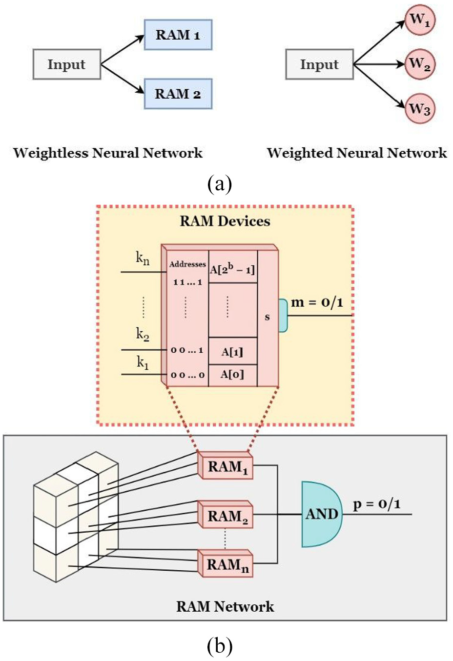
Aleksander pioneered the development of a groundbreaking digital neuron employing random access memory (RAM) components operating on Boolean logic, giving rise to a novel class of neural networks known as WNNs. In these networks, information was assimilated through the transmission of truth tables kept in the RAM. In the WNNs system, individual nodes were dedicated to identifying distinct portions of input patterns, given distinct addresses in the RAM. This established a mapping standard that could be supplied to the network in a binary configuration. In Figure 7(a), a vivid visual depiction is provided, illustrating the fundamental distinction between weighted and WNNs. RAM devices are the foundation of WNNs, storing essential image attributes through binary initialization, thus representing them as addresses. Conversely, weighted neural networks allocate weights across an entire spectrum of features. The pivotal benefit of utilizing a weightless neural network lies in its modeling and processing of the neural network itself. WNNs employ memory locations and hashing, while their weighted counterparts adjust signal strength between neurons through weighted synapses. In environments with limited memory resources, such as resource-constrained settings, WNNs are the preferred choice over their weighted counterparts. These characteristics position WNNs as an attractive option for specific real-world scenarios, especially those requiring minimal memory overheads for scalability and optimal performance. In our present study, the decision to employ WNNs was motivated by their low computational resource requirements and their potential suitability for real-time applications. In Figure 7(b), a basic depiction of a RAM network and neuron is presented, demonstrating how the network generates output values of either 0 or 1.

Figure 7.

(a) Working principle of weightless and weighted neural networks, highlighting the key differences in their operational mechanisms³⁵ and (b) schematic representation of the RAM network and its neuron structure, including the configuration of RAM devices used for processing.³⁵

WNNs with RAM components offer flexibility in design, with the WiSARD classifier being a particularly favored configuration. It incorporates multiple discriminators, each tailored to a specific class based on user-defined parameters. Figure 8 provides a visual representation of the WiSARD classifier, emphasizing the crucial discriminator module. Equipped with RAM components, this module handles the processing of input patterns. The number of RAM elements present in the discriminator module is established by the patterned model derived from the input patterns. These RAM elements extract sub-patterns from the input pattern, presenting them as pairs. In the testing phase, the RAM component identifies the memory location associated with each pair, generating the stored output value, which can be either 0 or 1. The class pattern is discerned based on the highest cumulative output yielded by the discriminator module.

Figure 8.

Overview of the WiSARD classifier architecture highlighting the discriminator module used for classification and pattern recognition.³⁵

Results and discussion

In this study, an experiment was conducted to assess the fault diagnosis capabilities of the WiSARD classifier in diagnosing air compressor faults. Initially, several features were extracted (statistical, histogram, and ARMA) from the collected vibration signals. Using the J48 decision tree algorithm, the most influential and significant features were then identified. After this feature selection process, the entire dataset was divided into training and testing sets, with an 80%–20% split ratio. The dataset acquired contained 375 samples corresponding to 75 samples per condition. The training dataset (300 samples) was used to train the WiSARD classifier while the test dataset (75 samples) was used to test the performance. A 10-fold cross-validation approach was utilized to assess the validation accuracy of the trained model. To achieve higher classification accuracies, several hyperparameters were fine-tuned to ascertain the optimal values. The selection of the hyperparameter values were based on the literature that utilized WiSARD classifier for fault diagnosis.^36,37 The experimental findings are presented in the subsequent sections. The overall process was performed using WEKA data mining software (GUI Interface) developed by University of Waikato.³⁸ The software was run in a personal computer with the following configuration: Windows 10, 8 GB RAM and Intel i5—11th gen processor.

Influence of altering the ‘bit number’

The ‘Bit Number’ refers to the length of the binary vectors used for encoding the input data and representing the discriminators. Increasing the ‘Bit Number’ results in longer binary vectors for the discriminators. Longer binary vectors can capture more detailed information about the input data, potentially leading to better discrimination between different classes. Tables 2 –4 represent the performance of the WiSARD classifier for varying bit number values corresponding to statistical, histogram, and ARMA features respectively. Here, V.A., T.A., and T.S.A. refer to Cross Validation Accuracy, Training Set Accuracy, and Test Set Accuracy respectively. The value demonstrating the highest levels of accuracy was chosen as the ideal setting, which remained constant as the hyperparameter adjustment progressed to the subsequent one. Aside from the bit number, all remaining parameters retained their default configurations. Following the acquired outcomes, a bit number of 32 was determined as the most effective value for Statistical, Histogram, and ARMA features correspondingly.

Table 2.

WiSARD classifier performance with varying bit number (statistical features).

Bit No.	T.A. (%)	V.A. (%)	T.S.A. (%)
4	98.0000 (0.23 s)	92.7333 (0.03 s)	92.5333 (0.05 s)
8	98.6000 (0.16 s)	95.0666 (0.02 s)	94.6666 (0.07 s)
16	98.6667 (0.14 s)	95.0666 (0.01 s)	97.3333 (0.04 s)
32	98.6667 (0.13 s)	94.7333 (0.03 s)	97.6000 (0.02 s)

Table 3.

WiSARD classifier performance with varying bit number (histogram features).

Bit No.	T.A. (%)	V.A. (%)	T.S.A. (%)
4	92.3333 (0.32 s)	90.6000 (0.06 s)	94.6667 (0.06 s)
8	92.7333 (0.24 s)	91.6666 (0.06 s)	94.9333 (0.05 s)
16	92.8666 (0.18 s)	93.0000 (0.05 s)	95.7333 (0.05 s)
32	94.4666 (0.16 s)	94.4666 (0.03 s)	96.5333 (0.03 s)

Table 4.

WiSARD classifier performance with varying bit number (ARMA features).

Bit No.	T.A. (%)	V.A. (%)	T.S.A. (%)
4	97.6666 (0.13 s)	95.5333 (0.03 s)	93.6000 (0.03 s)
8	98.9714 (0.10 s)	96.7333 (0.03 s)	94.6666 (0.03 s)
16	98.6667 (0.10 s)	96.6000 (0.02 s)	95.4666 (0.02 s)
32	98.6667 (0.08 s)	96.6666 (0.02 s)	95.7333 (0.01 s)

Tables 2 –4 demonstrate the performance of a WiSARD classifier across varying bit numbers (4, 8, 16, and 32) using three different feature sets namely, statistical, histogram and ARMA. Overall, the statistical features consistently achieved the highest Test Set Accuracy (T.S.A.) with the 32 bit number configuration yielding the peak T.S.A. of 97.6000%. Histogram features also performed well with 32 bit number reaching T.S.A. values of 96.5333%. ARMA features showed the lowest overall accuracy compared to the other feature sets though performance improved with increasing bit number, reaching a peak T.S.A. of 95.7333% at 32 bit number.

Influence of altering the ‘bleach confidence’

The ‘Bleach Confidence’ is a parameter that controls the process of discarding the weak discriminators during training. Increasing the bleach confidence threshold leads to more aggressive pruning of weak discriminators during training. Weak discriminators are the ones that do not match the input data well and do not provide reliable classification information. By increasing the bleach confidence, the classifier becomes more selective in retaining discriminators, resulting in a more compact and memory-efficient model. Tables 5 –7 display the performance of the WiSARD classifier for Stat features, Histogram, and ARMA features, respectively, as the bleach confidence hyperparameter is varied. The abbreviations V.A., T.A., and T.S.A. stand for Cross Validation Accuracy, Training Set Accuracy, and Test Set Accuracy respectively. The optimum value was determined by selecting the one that provided both the highest accuracy and the shortest model-building time in each table. This optimal value was then kept fixed while further tuning the hyperparameters for the subsequent experiments. Every parameter, except for bit number and bleach confidence, retained their default settings. While the bleach confidence was varied, the bit number was kept at 32 as per our previous hyperparameter tuning. After reviewing the obtained outcomes, values of 0.6 for Stat features, 0.9 for Histogram features, and 0.95 for ARMA features were identified as the most advantageous bleach confidence levels.

Table 5.

WiSARD classifier performance with varying bleach confidence (statistical features).

Bl. Con.	T.A. (%)	V.A. (%)	T.S.A. (%)
0.60	98.6667 (0.13 s)	94.4666 (0.03 s)	98.6667 (0.03 s)
0.70	98.6667 (0.12 s)	94.8000 (0.02 s)	97.3333 (0.03 s)
0.80	98.6667 (0.12 s)	94.7333 (0.02 s)	98.4000 (0.03 s)
0.90	98.6667 (0.11 s)	94.6666 (0.02 s)	98.1333 (0.03 s)
0.95	98.6667 (0.13 s)	94.4000 (0.03 s)	98.4000 (0.03 s)

Table 6.

WiSARD classifier performance with varying bleach confidence (histogram features).

Bl. Con.	T.A. (%)	V.A. (%)	T.S.A. (%)
0.60	96.3333 (0.16 s)	94.0666 (0.05 s)	96.7999 (0.05 s)
0.70	93.8666 (0.19 s)	94.3333 (0.04 s)	96.2666 (0.03 s)
0.80	93.8000 (0.18 s)	94.0666 (0.03 s)	96.2666 (0.04 s)
0.90	94.5333 (0.17 s)	93.8666 (0.04 s)	96.7999 (0.03 s)
0.95	94.7999 (0.18 s)	93.7333 (0.03 s)	95.7333 (0.03 s)

Table 7.

WiSARD classifier performance with varying bleach confidence (ARMA features).

Bl. Con.	T.A. (%)	V.A. (%)	T.S.A. (%)
0.60	98.6667 (0.08 s)	96.6666 (0.02 s)	95.4666 (0.03 s)
0.70	98.6667 (0.08 s)	96.5333 (0.02 s)	95.2000 (0.02 s)
0.80	98.6667 (0.07 s)	96.7333 (0.02 s)	95.2000 (0.02 s)
0.90	98.6667 (0.08 s)	96.4000 (0.03 s)	94.6667 (0.02 s)
0.95	94.6667 (0.13 s)	96.9333 (0.02 s)	96.8000 (0.02 s)

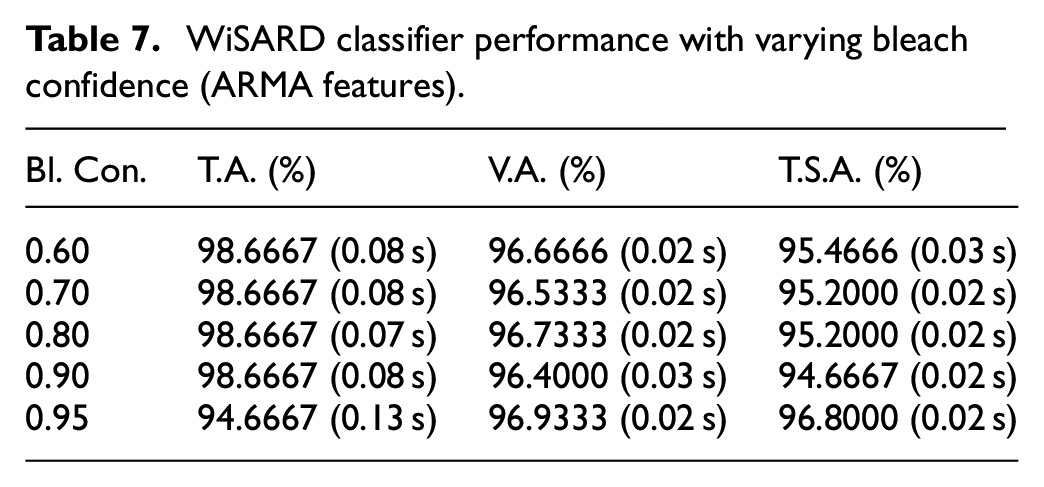
Tables 5 –7 demonstrate the performance of a WiSARD classifier across varying bleach confidence values (0.60–0.95). For statistical features, the T.A. remained consistently high at 98.6667% across all bleach confidence levels, with T.S.A also showing strong performance, peaking at 98.6667% at 0.60 bleach confidence. Histogram features exhibited T.S.A of 96.7999% at 0.9 bleach confidence. The ARMA features again showed the best performance with T.S.A. reaching 96.8000% at 0.95 bleach confidence.

Influence of altering the ‘bleach flag’

In the WiSARD classifier, the Bleach Flag is a parameter that determines whether or not weak discriminators should be discarded during the training process. When the bleach flag is set to true, the weak discriminators with activations below a certain threshold are removed from the classifier. On the other hand, when the bleach flag is set to false, all discriminators are retained regardless of their activation levels. The threshold is controlled by bleach confidence. Tables 8 –10 present the WiSARD classifier’s performance for Stat features, Histogram, and ARMA features, respectively, as the bleach flag hyperparameter is adjusted. Cross Validation Accuracy, Training Set Accuracy, and Test Set Accuracy are denoted by the acronyms V.A., T.A., and T.S.A. respectively. The optimum value was determined by selecting the one that provided both the highest accuracy and the shortest model-building time in each table. This optimal value was then fixed for subsequent experiments while tuning other hyperparameters. The parameters of bit number and bleach confidence were kept at their hyper-tuned values from the previous tuning and the bleach flag was varied between TRUE and FALSE. The other parameters were kept at their default values. Based on the results obtained, the bleach flag was selected FALSE as the optimal value for Stat, Histogram, and ARMA features respectively.

Table 8.

WiSARD classifier performance with varying bleach flag (statistical features).

Bl. Flag	T.A. (%)	V.A. (%)	T.S.A. (%)
TRUE	46.2000 (0.14 s)	54.6000 (0.02 s)	44.2666 (0.03 s)
FALSE	98.6667 (0.14 s)	94.4666 (0.02 s)	97.6000 (0.04 s)

Table 9.

WiSARD classifier performance with varying bleach flag (histogram features).

Bl. Flag	T.A. (%)	V.A. (%)	T.S.A. (%)
TRUE	93.6666 (0.19 s)	92.6666 (0.03 s)	89.6000 (0.02 s)
FALSE	95.5333 (0.17 s)	94.2666 (0.04 s)	97.0666 (0.03 s)

Table 10.

WiSARD classifier performance with varying bleach flag (ARMA features).

Bl. Flag	T.A. (%)	V.A. (%)	T.S.A. (%)
TRUE	65.9333 (0.10 s)	60.8000 (0.01 s)	56.5333 (0.01 s)
FALSE	98.6667 (0.13 s)	96.7333 (0.02 s)	96.0000 (0.02 s)

From Tables 8 to 10 one can observe that the accuracy for all feature sets reach a real low value when the bleach flag was set to TRUE. This indicates that FALSE will be the hyperparameter chose for the bleach flag for all the feature sets.

Influence of altering the ‘Bleach Step’

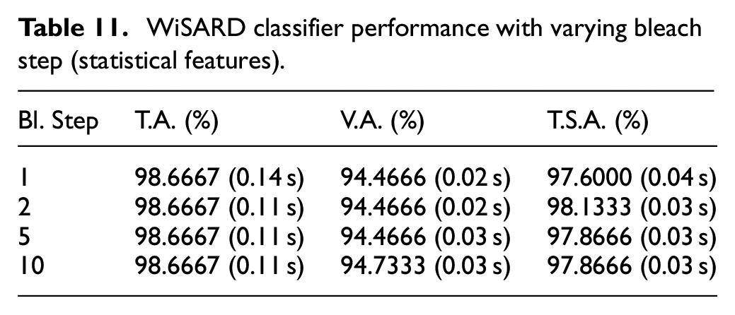
In the WiSARD classifier, the bleach step is the parameter that controls the frequency of discarding weak discriminators during the training process. A smaller bleach step value denotes the removal of weak discriminators more frequently during training. This speeds up the training process as the classifier continuously prunes less relevant discriminators, leading to a more efficient model-building process. Following are Tables 11 –13, which represent the performance of the WiSARD classifier as the bleach step is varied. The terms Cross Validation Accuracy (V.A.), Training Set Accuracy (T.A.), and Test Set Accuracy (T.S.A.) are used interchangeably with their respective abbreviations. The best-performing value in each table was determined by choosing the one that achieved the highest accuracy and required the least amount of time to construct the model. This optimal value was subsequently set as a fixed parameter for the following experiments, allowing further fine-tuning of other hyperparameters. Whilst all other parameters remained at their preset defaults, the bit number, the bleach confidence, and the bleach flag were kept at their hyper-tuned values and the bleach step was varied. Based on the results obtained as shown below, the bleach step selected 2.0, 10.0, and 2.0 as the optimal values for Stat, Histogram, and ARMA features respectively.

Table 11.

WiSARD classifier performance with varying bleach step (statistical features).

Bl. Step	T.A. (%)	V.A. (%)	T.S.A. (%)
1	98.6667 (0.14 s)	94.4666 (0.02 s)	97.6000 (0.04 s)
2	98.6667 (0.11 s)	94.4666 (0.02 s)	98.1333 (0.03 s)
5	98.6667 (0.11 s)	94.4666 (0.03 s)	97.8666 (0.03 s)
10	98.6667 (0.11 s)	94.7333 (0.03 s)	97.8666 (0.03 s)

Table 12.

WiSARD classifier performance with varying bleach step (histogram features).

Bl. Step	T.A. (%)	V.A. (%)	T.S.A. (%)
1	95.5333 (0.17 s)	94.2666 (0.04 s)	97.0666 (0.03 s)
2	97.1333 (0.17 s)	94.6000 (0.05 s)	96.5333 (0.04 s)
5	94.6666 (0.17 s)	94.0000 (0.03 s)	96.7999 (0.03 s)
10	95.5999 (0.19 s)	94.9999 (0.03 s)	97.0666 (0.02 s)

Table 13.

WiSARD classifier performance with varying bleach step (ARMA features).

Bl. Step	T.A. (%)	V.A. (%)	T.S.A. (%)
1	98.6667 (0.13 s)	96.7333 (0.02 s)	96.0000 (0.02 s)
2	98.6667 (0.09 s)	96.4666 (0.02 s)	96.2666 (0.02 s)
5	98.6667 (0.08 s)	96.8000 (0.01 s)	95.7333 (0.01 s)
10	98.6667 (0.08 s)	96.8000 (0.02 s)	94.9333 (0.01 s)

Tables 11 –13 demonstrate the performance of a WiSARD classifier across varying bleach step values (1, 2, 5, and 10). For statistical features, the T.A. remained consistently high at 98.6667% across all bleach step levels, with T.S.A also showing strong performance, peaking at 98.1333% at two bleach step. Histogram features exhibited T.S.A of 97.0666% at 10 bleach step while the ARMA features again showed the best performance with T.S.A. reaching 96.2666% at two bleach step.

Influence of altering the ‘map type’

The Map Type parameter in the WiSARD classifier determines how input patterns are mapped to discriminator fields. There are two types of mapping in this classifier, namely Random, and Linear. In Linear mapping, each input pattern is mapped to a discriminator field using a deterministic, systematic method. This results in discriminators of fixed and equal length, ensuring consistent sizes across the classifier. In Random mapping, each input pattern is mapped to a discriminator field with a randomly generated binary vector. The length of this binary vector can vary across different discriminator fields, leading to discriminators of different sizes. Linear mapping provides a systematic and predictable representation of the input patterns while Random mapping allows for more flexibility in the representation of patterns, capturing a broader range of patterns in the input data. Tables 14 –16 display the performance of the WiSARD classifier as the bleach step hyperparameter is adjusted. V.A., T.A., and T.S.A. represent Cross Validation Accuracy, Training Set Accuracy, and Test Set Accuracy, in that order. To identify the best-performing value, we selected the one that achieved the highest accuracy and required the shortest model construction time in each table. This optimal value was then fixed as a parameter for subsequent experiments, enabling further refinement of other hyperparameters. The parameters of bleach confidence, bit number, bleach step, and bleach flag were kept as their tuned values and the map type was varied. All other parameters remained at their preset defaults. Based on the results obtained as shown below, the Random map type was selected for all of the different features.

Table 14.

WiSARD classifier performance with varying map type (statistical features).

Map type	T.A. (%)	V.A. (%)	T.S.A. (%)
RANDOM	98.6667(0.11 s)	94.5333(0.02 s)	98.6667(0.03 s)
LINEAR	98.6667(0.05 s)	92.6667(0.01 s)	96.0000(0.02 s)

Table 15.

WiSARD classifier performance with varying map type (histogram features).

Map type	T.A. (%)	V.A. (%)	T.S.A. (%)
RANDOM	93.9333(0.19 s)	94.0000(0.03 s)	96.7999(0.02 s)
LINEAR	97.3333(0.13 s)	89.0000(0.02 s)	96.0000(0.02 s)

Table 16.

WiSARD classifier performance with varying map type (ARMA features).

Map type	T.A. (%)	V.A. (%)	T.S.A. (%)
RANDOM	98.6667(0.08 s)	96.4666(0.02 s)	96.2666(0.01 s)
LINEAR	97.6667(0.08 s)	90.0000(0.01 s)	85.3333(0.01 s)

From Tables 14 to 16 one can observe that the T.S.A for all feature sets reach a real higher values when the map type was set to RANDOM. This indicates that RANDOM will be the hyperparameter chose for the map type for all the feature sets.

Influence of altering the ‘Tic Number’

The Tic Number in the WiSARD classifier is a parameter that controls the number of times the classifier processes the input data during the training process. Increasing the tic number lets the classifier process the input data given multiple times during training. This repetitive exposure to the data improves the model convergence and represents the patterns better in the data. But there’s also an increase in overall training time for a larger tic number. Tables 17 –19 provide a clear insight into this variation of tic number and its impact on the input data. Referring to Cross Validation Accuracy, Training Set Accuracy, and Test Set Accuracy, V.A., T.A., and T.S.A. are the respective abbreviations. All the previously tuned hyperparameters had been kept at their optimal values and the rest of the remaining were kept at their default values. Only the tic number was varied. Based on the results obtained, 100, 256, and 256 were kept as the optimal values of the tic number for Stat, Histogram, and ARMA Features respectively.

Table 17.

WiSARD classifier performance with varying tic number (statistical features).

Tic No.	T.A. (%)	V.A. (%)	T.S.A. (%)
1	20.6667 (0.01 s)	19.3333 (0.00 s)	18.6667 (0.00 s)
10	72.6000 (0.02 s)	66.0666 (0.01 s)	68.0000 (0.01 s)
20	92.3999 (0.05 s)	85.0000 (0.01 s)	87.6000 (0.01 s)
50	98.0000 (0.05 s)	93.3333 (0.01 s)	93.6000 (0.01 s)
100	98.6667 (0.07 s)	94.2000 (0.01 s)	98.1333 (0.01 s)
256	98.6667 (0.11 s)	94.6666 (0.02 s)	98.6667 (0.03 s)

Table 18.

WiSARD classifier performance with varying tic number (histogram features).

Tic No.	T.A. (%)	V.A. (%)	T.S.A. (%)
1	26.6667 (0.00 s)	21.6000 (0.00 s)	20.0000 (0.00 s)
10	71.6000 (0.01 s)	68.5333 (0.00 s)	66.1333 (0.00 s)
20	77.3333 (0.03 s)	75.2666 (0.01 s)	74.1333 (0.01 s)
50	90.0666 (0.04 s)	89.8666 (0.02 s)	93.0666 (0.01 s)
100	90.6666 (0.08 s)	91.4666 (0.02 s)	93.0666 (0.01 s)
256	95.5999 (0.19 s)	94.0000 (0.03 s)	96.7999(0.02 s)

Table 19.

WiSARD classifier performance with varying tic number (ARMA features).

Tic No.	T.A. (%)	V.A. (%)	T.S.A. (%)
1	20.6667 (0.00 s)	20.3333 (0.00 s)	20.0000 (0.00 s)
10	82.2666 (0.00 s)	76.8666 (0.00 s)	65.8666 (0.00 s)
20	84.0000 (0.02 s)	84.3380 (0.01 s)	82.1333 (0.01 s)
50	96.2000 (0.03 s)	94.5333 (0.01 s)	93.8666 (0.01 s)
100	98.6667 (0.04 s)	96.5333 (0.01 s)	95.1999 (0.01 s)
256	98.6667 (0.08 s)	96.6000 (0.02 s)	95.4666 (0.01 s)

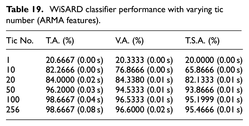
Tables 17 –19 demonstrate the performance of a WiSARD classifier across varying tic number values (1, 10, 20, 50, 100, and 256). For statistical features, the T.S.A at 256 tic number reached 98.6667%. Histogram and ARMA features exhibited T.S.A of 96.7999% and 95.4666% respectively at 256 tic number. It can also be observed that the values of accuracy dropeed significantly when the tic number was reduced.

Ideal hyperparameter selection

Table 20 showcases the best hyperparameter choices derived from the comprehensive research conducted in the aforementioned sections for statistical, histogram, and ARMA features, respectively. Model effectiveness was assessed using the best-performing hyperparameters, and the resulting performance was gaged using the depicted confusion matrix in Figures 9 –11 for Statistical Features, Histogram Features, and ARMA Features respectively. A confusion matrix serves as a structured representation to assess how well a classification algorithm performs. It compiles algorithm predictions on a test dataset, contrasting these predictions against actual labels for evaluation purposes. These matrices depict a multi-category classification, distinguishing between compromised and intact suspension systems, respectively. This research underscores the importance of utilizing the WiSARD classifier for precise categorization of the various types of features. Furthermore, the research effectively showcased the efficiency of the suggested approach for fault diagnosis, employing the WiSARD classifier.

Table 20.

Ideal hyperparameters for WiSARD classifier.

Hyperparameter	Statistical	Histogram	ARMA
Bit No.	32	32	32
Bl. Con.	0.60	0.90	0.95
Bl. flag	False	False	False
Bl. step	2	10	2
Map type	Random	Random	Random
Tic No.	256	256	256
Classificationaccuracy (%)	98.6667	96.7999	95.4666

Figure 9.

Confusion matrix illustrating the performance of the WiSARD classifier with optimized hyperparameters, evaluated using statistical features for classification accuracy.

Figure 10.

Confusion matrix illustrating the performance of the WiSARD classifier with optimized hyperparameters, evaluated using histogram features for classification accuracy.

Figure 11.

Confusion matrix illustrating the performance of the WiSARD classifier with optimized hyperparameters, evaluated using ARMA features for classification accuracy.

From Figure 9, one can identify that one instance of PRV was misclassified as IVF. This observation suggests that the classifier was unable to distinguish between PRV and IVF due to the possible overlap in the feature distribution or similarity in the signal characteristics. On the other hand, in Figure 10, one instance of GOOD was misclassified as IOVF, IVF as GOOD and PRV as IVF. The possible reasons for such misclassification might be due to the lack of sufficient number of discriminative features among these classes. From Figure 11, it can be observed that two instances of IVF were misclassified as GOOD and one instance each of OVF, PRV, and IOVF being misclassified as IVF, IVF and OVF respectively. The higher number of misclassifications in IVF suggests that there might be a potential overlap of signals or features in the GOOD class. Some suggestions to improvise the classification performance and reduce misclassifications can be enhancing the training data, additional feature engineering, refining class boundaries, model fine tuning, and adjusting the feature selection.

Conclusions

Condition monitoring using vibration analysis was conducted on an air compressor system, examining its performance across five distinct test scenarios. The study involved the extraction of various attributes, including ARMA, histogram, and statistical features. The J48 decision tree technique was utilized to pinpoint the features of utmost significance. These distinctive attributes from each extracted feature were utilized as input for classification through the WiSARD classifier. The evaluation focused on the classification accuracy obtained from the WiSARD classifier. In order to attain the highest possible output and minimize the model-building duration, numerous hyperparameters underwent testing to identify the most advantageous configuration. The results obtained demonstrate that the WiSARD classifier when combined with statistical features attains an accuracy of 98.67% with the optimal hyperparameter settings. These findings imply that the model created utilizing the WiSARD classifier and statistical features can be integrated into real-time applications for diverse fault classifications. While the WiSARD classifier offers advantages such as low computational resource requirements and fast training, it has certain limitations including sensitivity to high-dimensional data and noisy inputs which may lead to misclassifications. Its scalability with large datasets and adaptability to raw data remain challenging as it relies on predefined features. Additionally, class imbalance can affect performance thereby requiring techniques like synthetic data generation to improve results. This implementation holds the potential to enhance the longevity, dependability, and safety of air compressors by providing immediate results. Computational efficient and cost-effective solutions have a great potential in the future to attract interest among research community and industrial scenarios.

Footnotes

Handling Editor: Chaoqun Duan

ORCID iD

Naveen Venkatesh Sridharan

Funding

The author(s) received no financial support for the research, authorship, and/or publication of this article.

Declaration of conflicting interests

The author(s) declared no potential conflicts of interest with respect to the research, authorship, and/or publication of this article.

Data availability statement

Data will be made available on request.

References

AlShorman

Irfan

Saad

, et al. A review of artificial intelligence methods for condition monitoring and fault diagnosis of rolling element bearings for induction motor. Shock Vib 2020; 2020: 1–20.

Kim

Lee

, et al. Effective band-selection algorithm for rolling element bearing diagnosis using AE sensor data under noisy conditions. Struct Multidiscipl Optim 2022; 65: 1–23. DOI: 10.1007/S00158-022-03360-4.

Zhiyi

Haidong

Xiang

, et al. An intelligent fault diagnosis method for rotor-bearing system using small labeled infrared thermal images and enhanced CNN transferred from CAE. Adv Eng Inform 2020; 46: 101150.

Wang

, et al. Industrial gearbox fault diagnosis based on multi-scale convolutional neural networks and thermal imaging. ISA Trans 2022; 129: 309–320.

Wan

, et al. Rotating machinery fault diagnosis based on convolutional neural network and infrared thermal imaging. Chin J Aeronaut 2020; 33: 427–438.

Sun

Wang

, et al. Online oil debris monitoring of rotating machinery: A detailed review of more than three decades. Mech Syst Signal Process 2021; 149: 107341.

Pradhan

Mishra

. Analysis of ISO VG 68 bearing oil for condition monitoring collected from an externally pressurized ball bearing system. Mater Today Proc 2021; 44: 4602–4606.

Verellen

Verbelen

Stockman

, et al. Beamforming applied to ultrasound analysis in detection of bearing defects. Sensors 2021; 21: 1–13. DOI: 10.3390/S21206803.

Ishak

Yaw

Koh

, et al. Fault classification system for switchgear cbm from an ultrasound analysis technique using extreme learning machine. Energies 2021; 14: 6279.

10.

Glowacz

Tadeusiewicz

Legutko

, et al. Fault diagnosis of angle grinders and electric impact drills using acoustic signals. Appl Acoust 2021; 179: 108070.

11.

AlShorman

Alkahatni

Masadeh

, et al. Sounds and acoustic emission-based early fault diagnosis of induction motor: A review study. Adv Mech Eng 2021; 13: 1–19. DOI: 10.1177/1687814021996915/ASSET/IMAGES/LARGE/10.1177_1687814021996915-FIG5.JPEG.

12.

Ribeiro Junior

Areias

IADS

Gomes

. Fault detection and diagnosis using vibration signal analysis in frequency domain for electric motors considering different real fault types. Sens Rev 2021; 41: 311–319.

13.

Pan

Zhao

Song

, et al. Research on gear fault diagnosis based on feature fusion optimization and improved two hidden layer extreme learning machine. Measurement 2021; 177: 109317.

14.

Liang

Tong

. Fault diagnosis techniques for Nuclear Power Plants: A review from the Artificial Intelligence Perspective. Energies 2023; 16: 1850.

15.

Kumar

Gandhi

Vashishtha

, et al. VMD based trigonometric entropy measure: a simple and effective tool for dynamic degradation monitoring of rolling element bearing. Meas Sci Technol 2022; 33: 014005.

16.

Cui

Guan

Chen

. Rolling Element Fault diagnosis based on VMD and sensitivity MCKD. IEEE Access 2021; 9: 120297–120308.

17.

Tran

AlThobiani

Tinga

, et al. Single and combined fault diagnosis of reciprocating compressor valves using a hybrid deep belief network. Proc IMechE, Part C: J Mechanical Engineering Science 2018; 232: 3767–3780.

18.

Mohan

. An analysis of air compressor fault diagnosis using machine learning technique. J Mech Contin Math Sci 2019; 14: 13–27. DOI: 10.26782/JMCMS.2019.12.00002.

19.

Liu

Duan

Yuan

, et al. An intelligent fault diagnosis method for reciprocating compressors based on LMD and SDAE. Sensors 2019; 19: 1041.

20.

Tang

Lin

. Fault feature extraction of reciprocating compressor based on adaptive waveform decomposition and Lempel-Ziv complexity. IEEE Access 2019; 7: 82522–82531.

21.

Prashanth

Elangovan

. Vibration based fault monitoring of a compressor using tree-based algorithms. IOP Conf Ser Mater Sci Eng 2019; 577: 012116.

22.

Ravikumar

Kanagasabapathy

Muralidharan

. Fault diagnosis of self-aligning troughing rollers in belt conveyor system using k-star algorithm. Measurement 2019; 133: 341–349.

23.

Tong

Wang

, et al. A novel pipeline leak recognition method of mine air compressor based on infrared thermal image using IFA and SVM. Appl Sci 2020; 10: 5991.

24.

Joshuva

Sugumaran

. Crack detection and localization on wind turbine blade using machine learning algorithms: a data mining approach. Struct Durab Heal Monit 2019; 13: 181–203.

25.

Lei

. EEMD method and WNN for fault diagnosis of locomotive roller bearings. Expert Syst Appl 2011; 38: 7334–7341.

26.

De Souza

Freitas

De Almeida

AGC

. High performance prediction of stock returns with VG-RAM weightless neural networks. In: 2010 IEEE workshop on high performance computational finance, 2010. DOI: 10.1109/WHPCF.2010.5671832.

27.

Doquire

Michel

. Mutual information for feature selection with missing data. In: ESANN 2011: 19th European symposium on artificial neural networks, computational intelligence and machine learning, 2011: proceedings, Bruges, Belgium, 27–29 April 2011, p.509.

28.

McElroy

Howells

. Automated adaptation of input and output data for a weightless artificial neural network. Int J Database Theory Appl 2011; 4: 49–58.

29.

De Gregorio

Giordano

. Change detection with weightless neural networks. In: IEEE computer society conference on computer vision and pattern recognition workshops, 2014, pp.409–413.

30.

Yin

Costa

JAF

Barreto

. Intelligent Data Engineering and Automated Learning - IDEAL 2012. 7435. 2012. DOI: 10.1007/978-3-642-32639-4.

31.

Amarnath

Sugumaran

Kumar

. Exploiting sound signals for fault diagnosis of bearings using decision tree. Measurement 2013; 46: 1250–1256.

32.

Joshuva

Sugumaran

. A lazy learning approach for condition monitoring of wind turbine blade using vibration signals and histogram features. Measurement 2020; 152: 107295.

33.

Said

Dickey

. Testing for unit roots in autoregressive-moving average models of unknown order. Biometrika 1984; 71: 599.

34.

Sugumaran

Muralidharan

Ramachandran

. Feature selection using decision tree and classification through proximal support vector machine for fault diagnostics of roller bearing. Mech Syst Signal Process 2007; 21: 930–942.

35.

Sridharan

Joseph

Vaithiyanathan

, et al. Weightless neural network-based detection and diagnosis of visual faults in photovoltaic modules. Energies 2023; 16: 5824.

36.

Shah

Venkatesh

Balaji

, et al. Weightless neural network-based fault diagnosis in suspension system. FME Trans 2024; 52: 115–127.

37.

Shah

Sridharan

Ramasamy

, et al. Monitoring the condition of monoblock centrifugal pumps using vibration analysis and WiSARD classifier. J Braz Soc Mech Sci Eng 2025; 47: 18.

38.

Hall

Frank

Holmes

, et al. The WEKA data mining software. ACM SIGKDD Explor Newsl 2009; 11: 10–18.

Detection and diagnosis of air compressor faults using weightless neural networks

Abstract

Keywords

Introduction

The novelty of the present study

The primary contributions of this study are outlined as follows

Experimental studies

Experimental setup

Experimental procedure

Process of extraction of features

Extraction of statistical feature

Extraction of histogram features

Extraction of ARMA features

Process of selection of features

WNN based feature classification process (WiSARD classifier)

Results and discussion

Influence of altering the ‘bit number’

Influence of altering the ‘bleach confidence’

Influence of altering the ‘bleach flag’

Influence of altering the ‘Bleach Step’

Influence of altering the ‘map type’

Influence of altering the ‘Tic Number’

Ideal hyperparameter selection

Conclusions

Footnotes

ORCID iD

Funding

Declaration of conflicting interests

Data availability statement

References