Sage Journals: Discover world-class research

Abstract

Stability and steering comfort are improved using an Electric Power Steering (EPS) system instead of a traditional Hydraulic Power Steering (HPS) system. A new control algorithm is proposed in this work to control automotive EPS systems. The proposed algorithm solves two main existing problems: eliminating the influence of systematic errors and ensuring tracking for all state variables instead of just a single object. This algorithm is formed based on a combination of Fuzzy and Linear Quadratic Tracking control techniques, so it is called FLQT. The proposed fuzzy technique has two inputs, angle error, and rate error, which are used to correct the input signal of the LQT technique and reduce systematic error. Simulation results are obtained from specific cases corresponding to two types of driver torques. The article shows that when the FLQT algorithm controls the system, the Root Mean Square (RMS) error does not go over 0.021% (in the first case) or 0.057% (in the second case). However, conventional LQT and Proportional-Integral-Derivative (PID) techniques can increase the RMS error to 18.809% and 42.543%, respectively. System stability and adaptability are guaranteed even when vehicle speed and driver torque change.

Keywords

Electric power steering linear quadratic tracking fuzzy control steering column angle steering motor angle

Introduction

A Power-Assisted Steering (PAS) system provides assisted torque to reduce steering effort when a vehicle moves on a road. This system was invented in the 1950s of the last century and is still used today. There are two commonly used assisted steering methods, including electric-assisted steering and hydraulic-assisted steering.¹ A combination of electric steering and hydraulic steering is called Electrohydraulic Power Steering (EHPS).² The EPS system offers many outstanding advantages compared to the traditional HPS system. Allous et al.³ showed that the weight of the EPS system is much smaller than that of the HPS. The size of the EPS system is relatively compact so that it can be easily installed on the vehicle. In addition, the EPS system operates independently of the combustion engine.⁴ Wang and Karimi⁵ mentioned that the EPS system could reduce carbon dioxide emissions by reducing fuel consumption. Ramasamy also concluded that energy consumption efficiency was improved by about 3% when replacing the traditional HPS system with the EPS system.⁶ Additionally, the EPS system is more environmentally friendly than HPS and EHPS because it does not require hydraulic oil. In addition, system noise is significantly improved when replacing classic PAS systems with modern EPS systems.⁶ Finally, the EPS system’s power steering and adaptability are superior to other systems. This is guaranteed even when the vehicle moves at low or extremely high speeds. With the above outstanding advantages, EPS systems are equipped on most types of vehicles today, such as family cars,⁷ forklifts,⁸ terrain vehicles,⁹ and others. There are three basic configurations of EPS systems widely used today: column steering (C-EPS), pinion steering (P-EPS), and rack steering (R-EPS). Type C-EPS is often applied to small and medium-sized vehicles, while the other two are used on larger vehicles.¹⁰

Control algorithms for EPS systems are designed based on the researcher’s perspective and each specific target. Hassan et al.¹⁰ designed a simple PID controller to control a motor current. The parameters of this controller were tuned by a binary-coded genetic algorithm. This algorithm’s goal was to make the RMS error converge to zero. However, the error between optimized parameters and non-optimized parameters was not significant. An Ant Colony Optimization (ACO) technique was introduced by Hanifah et al.¹¹ to search for optimal values for the controller of the EPS system. Similar to Hassan et al.,¹⁰ the target of the algorithm proposed in Hanifah et al.¹¹ was also to reduce the RMS error to reduce power consumption. These values converged after about 20 iterations with no significant error. However, the power consumption decreased slightly, from 25.02 to 24.98 A. A precise compound control method for loading rack force was presented by Dai et al.¹² This method was formed based on the combination of PI and fuzzy techniques. The fuzzy controller’s output was the system error (input to the PI controller). In many survey situations, the phase shift phenomenon frequently occurs. Zheng and Wei designed a fuzzy PI controller to solve this problem.¹³ The parameters of the PI controller in Zheng and Wei¹³ were dynamically adjusted by a fuzzy technique. Simulation results showed that the overshoot phenomenon decreased from 6.6% to 2.2% when the Active Disturbance Rejection Control (ADRC) was replaced with the FPI technique. To improve the delay margin, Diab et al. designed a linear assistance filter for the EPS system.¹⁴ However, the systematic error obtained from this method was relatively large. An integrated PID-PI controller was introduced by Manca et al.¹⁵ Simulation results showed that the output signals were affected by chattering, while phase shifts occurred as the frequency increased. Li et al.¹⁶ designed the Backpropagation Neural Network (BPNN) algorithm to tune parameters for the PID controller of the EPS system. The system responded well when steering at high speed. However, a phase delay occurred when the vehicle steered at low speed. Ramos-Fernández designed an intelligent self-learning algorithm, the Adaptive Neuro-Fuzzy Inference System (ANFIS), to train the control model of the EPS system. The training data was taken from a conventional PD controller. Simulation results showed that the systematic error was relatively large.¹⁷ Regarding heavy vehicles, the use of two independent electric motors is necessary. They can be controlled by two independent PID algorithms.^18,19 The PID technique is a simple method and is often applied in industry. However, this technique can only be applied to Single Input and Single Output (SISO) systems. Under some conditions, the systematic error is considerable even when the parameters have been optimally calculated.

Several robust control methods have also been applied to EPS systems. Khasawneh and Das²⁰ designed a Sliding Mode Control (SMC) algorithm to control the steering system. The systematic error was reduced when this technique was applied. However, the chattering phenomenon was strong. A robust nonlinear algorithm to control Steering Wheel Torque (SWT) was established by Kim et al.²¹ An Extended State Observer (ESO) was integrated with the SMC technique to eliminate the influence of uncertainties and external disturbances. Simulation results in Kim et al.²¹ showed that the output signal tended to follow the reference signal with acceptable errors. However, the actual signals were strongly chattered. An adaptive SMC method was introduced by Lee et al.²² Like Kim et al.,²¹ the object that needed to be controlled in Lee et al.²² was SWT. Under the control of adaptive SMC technology, the steering wheel angle closely followed the reference value, but the steering wheel rate and acceleration error were quite large. Additionally, the steering wheel rate and acceleration output signals underwent intense chattering. The reason was that they were not controlled objects. A significant improvement was seen in the results when combining the fuzzy technique with adaptive SMC to become AFSMC.²³ However, this was only true for the controlled object (motor current). To eliminate the influence of external factors, Na et al. applied the ADRC technique to the EPS system based on the SWT tracking target.²⁴ The computational results in Na et al.²⁴ showed that the angle error was relatively small, but the angular speed error was strongly chattered below the sinusoidal response. According to Zheng and Wei, the ADRC algorithm performs better than fuzzy PID in reducing overshoot. However, the output signals still underwent chattering.²⁵ A combination of PI and Backstepping Control (BSC) was shown by Nguyen and Nguyen.²⁶ The control signal calculation process in Nguyen and Nguyen²⁶ was highly complicated. Therefore, they used an approximate calculation method to simplify this work. As a result, errors and phase shifts in the signal increased. To solve this problem, the input signal of the backstepping controller was calibrated using the PI technique. An improvement of Nguyen and Nguyen²⁶ was mentioned in Nguyen²⁷ based on a fuzzy technique used to tune the parameters of the PI-BSC controller dynamically. Although robust control techniques can effectively reduce systematic errors, they are usually only applied to SISO systems. The algorithm will become highly complex once these techniques are applied to Multi-Input and Multi-Output (MIMO) systems. In addition, the chattering phenomenon can occur more intensely due to system interaction when applying SMC and ADRC techniques to many state variables.

The Linear Quadratic Regulator (LQR) technique provides high efficiency in controlling MIMO systems.²⁸ This linear control method does not cause chattering like the abovementioned nonlinear control methods. Chitu et al.²⁹ designed a digital LQR algorithm to control the EPS system model. This algorithm was described in terms of state spaces. Irmer and Henrichfreise³⁰ introduced a control mechanism based on the combination of a Linear Quadratic Regulator (LQR), a Linear Quadratic Gaussian (LQG), and a Linear Quadratic Estimation (LQE). However, the structure of the algorithms in Chitu et al.²⁹ and Irmer and Henrichfreise³⁰ was not explicitly presented. A Kalman filter was integrated with the LQR technique to limit the influence of disturbances.³¹ Liu et al.³² introduced an optimal fault-tolerant controller based on LQR and GA techniques. However, they only evaluated impulse and step response results without other state variables. The traditional LQR algorithm is often applied to models with zero reference signals, such as active suspension or active anti-roll systems. This algorithm must be transformed into Linear Quadratic Tracking (LQT) to control the object and ensure it follows a predetermined trajectory. This method is only suitable for classical linear systems, which are not affected by disturbances. The systematic error will increase once the influence of disturbances increases. This is considered a limitation when applying LQR and LQT techniques to control systems.

The above literature review shows that some problems still exist: (1) The PID technique can only be applied to SISO systems. Therefore, the systematic error is significant for uncontrolled state variables.^14–17 In addition, the overshoot phenomenon still exists even when the parameters have been optimally calculated¹³; (2) Nonlinear control techniques (such as BSC, SMC, and ADRC) can provide high performance in eliminating systematic errors. However, the output signals are greatly affected by chattering and can cause adverse impacts on the system.^{20–22,24,25} If these techniques are applied to MIMO systems, the effect of chattering can be further increased; (3) Some LQR techniques mentioned in References 29–32 are pretty simple, leading to increased systematic errors; (4) The energy consumption of some controllers is relatively large^11,33; (5) The calculation of road reaction torque value is omitted³⁴ or calculated in a simplified way.³⁵

To solve the above problems, we propose to design a Linear Quadratic Tracking (LQT) algorithm to control the state variables of the MIMO system. The input of the LQT technique is calibrated through two fuzzy controllers to reduce systematic errors. The fuzzy algorithm offers many advantages in solving nonlinear and highly uncertain problems. In addition, it provides efficient handling of models affected by disturbances and noise. The fuzzy algorithms are formulated without determining the object model, which is required for other control methods. This combination helps solve problems 1–4. The fifth problem is solved by establishing a dynamic model to describe the vehicle’s motion to calculate the road reaction torque value. These are considered new contributions to the article. The structure of this article is divided into four sections. Literature review and work motivation are mentioned in the first section. The second section presents the design of the system model and control algorithm. The following section covers the numerical simulation results and discussion. Finally, some comments and future development directions are indicated in the conclusion section.

Mathematical model

C-EPS system model

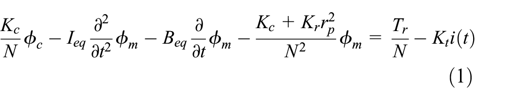
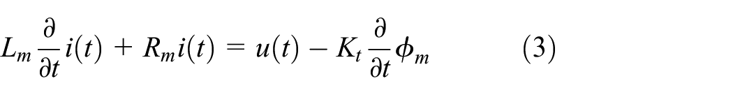
The structure of the C-EPS system is illustrated in Figure 1(a). The relationship between steering column angle (ϕ_c), steering motor angle (ϕ_m), and motor current (i_m) is described by equations (1)–(3).

Figure 1.

System models: (a) C-EPS model and (b) vehicle model.

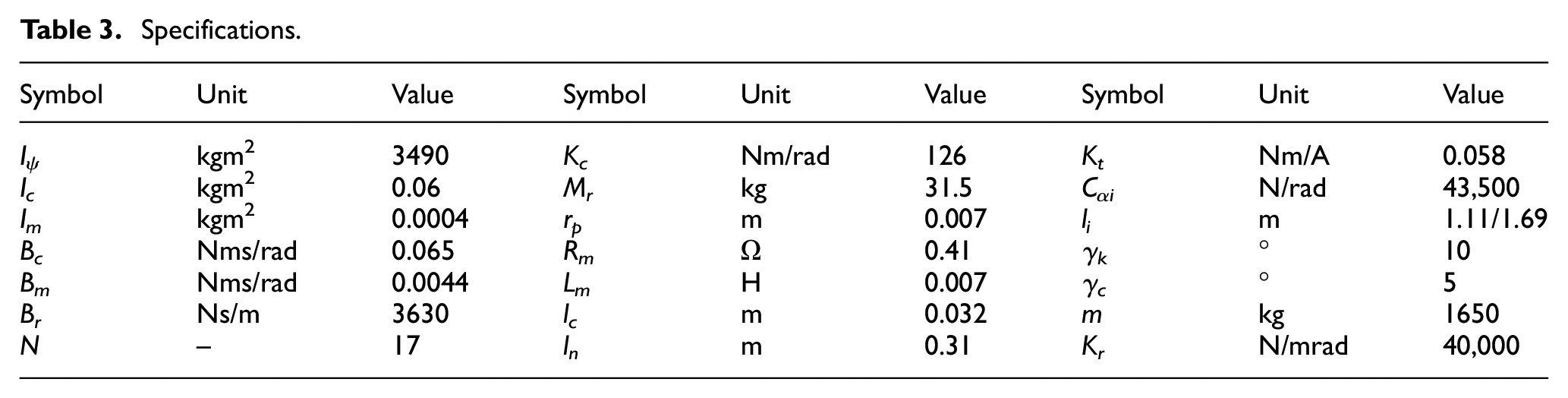
The symbols used for this equation include I_c and I_m are the inertia moment of the steering column and steering motor, respectively; B_c, B_m, and B_r are steering column damping, steering motor damping, and rack damping, respectively; N is motor ratio, K_t is motor torque coefficient, K_c is torsional stiffness of the steering column, T_d is driver torque, M_r is rack mass, K_r is rate coefficient, r_p is pinion radius, R_m is motor resistance, and L_m is motor inductance.

\frac{K_{c}}{N} ϕ_{c} - I_{eq} \frac{\partial^{2}}{\partial t^{2}} ϕ_{m} - B_{eq} \frac{\partial}{\partial t} ϕ_{m} - \frac{K_{c} + K_{r} r_{p}^{2}}{N^{2}} ϕ_{m} = \frac{T_{r}}{N} - K_{t} i (t)

(1)

I_{c} \frac{\partial^{2}}{\partial t^{2}} ϕ_{c} + B_{c} \frac{\partial}{\partial t} ϕ_{c} + K_{c} ϕ_{c} - \frac{K_{c}}{N} ϕ_{m} = T_{d}

(2)

L_{m} \frac{\partial}{\partial t} i (t) + R_{m} i (t) = u (t) - K_{t} \frac{\partial}{\partial t} ϕ_{m}

(3)

The equivalent damping coefficient (B_eq) and equivalent moment of inertia (I_eq) are calculated according to equations (4) and (5), respectively.

B_{eq} = B_{m} + \frac{r_{p}^{2}}{N^{2}} B_{r}

(4)

I_{eq} = I_{m} + \frac{r_{p}^{2}}{N^{2}} M_{r}

(5)

Road reaction torque (T_r) is the sum of two components: steering resistance torque (T_sr) and road disturbances (T_rd), that is, T_r = T_sr + T_rd. The calculation of steering resistance torque (T_sr) follows equation (6), where l_c is the caster trail; l_n is knuckle arm length; F_y is lateral tire force; γ_c and γ_k are caster and kingpin angles, respectively. The change in road disturbances (T_rd) is considered one of the known simulation inputs and will be mentioned in the following section.

T_{sr} = l_{c} r_{p} \frac{co s^{2} γ_{k} co s^{2} γ_{c}}{l_{n}} F_{y 1}

(6)

Lateral tire forces are calculated based on tire models. Nonlinear tire models (such as the Pacejka, Burckhard, and others) provide accurate calculations under complex conditions. However, these models are tricky because they need many nonlinear equations and experimental parameters.³⁶ A linear tire model is used instead of complex nonlinear models to simplify calculations. Assuming that the tire is deformed in the linear area (the steering angle is small enough), the lateral force at the front and rear tires are calculated according to (7) and (8), respectively.

F_{y 1} = - C_{α 1} α_{1}

(7)

F_{y 2} = - C_{α 2} α_{2}

(8)

The cornering stiffness of the tire (C_α) is a predetermined constant. Therefore, the value of the lateral force depends almost linearly on the slip angle (α). The relationship between slip angle (α), steering angle (δ), yaw angle (ψ), longitudinal velocity (v_x), and lateral velocity (v_y) is described by equations (9) and (10).

α_{1} = \frac{v_{y} + l_{1} \frac{\partial}{\partial t} ψ}{v_{x}} - δ

(9)

α_{2} = \frac{v_{y} - l_{2} \frac{\partial}{\partial t} ψ}{v_{x}}

(10)

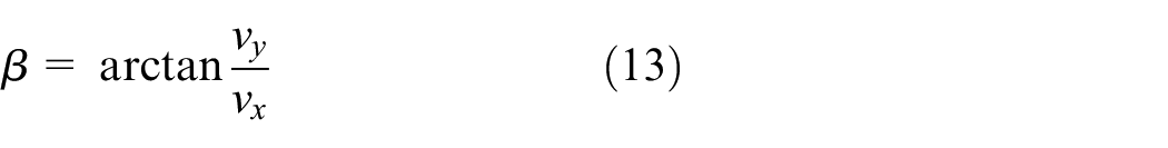
According to equations (11) and (12), the longitudinal velocity and lateral velocity are calculated based on the heading angle (β). The relationship between these two quantities can be rewritten as (13).

v_{x} = v \cos β

(11)

v_{y} = v \sin β

(12)

β = \arctan \frac{v_{y}}{v_{x}}

(13)

Yaw angle (ψ) is a solution of equations (14)–(16). These equations are established based on a single-track dynamics model (Figure 1(b)). The number of unknowns in these equations is more than the number of equations, so it is difficult to find their solutions.

m (\frac{\partial}{\partial t} v_{x} - v_{y} \frac{\partial}{\partial t} ψ) = F_{x 1} \cos δ + F_{x 2} - F_{y 1} \sin δ

(14)

m (\frac{\partial}{\partial t} v_{y} + v_{x} \frac{\partial}{\partial t} ψ) = F_{y 1} \cos δ + F_{y 2} + F_{x 1} \sin δ

(15)

I_{ψ} \frac{\partial^{2}}{\partial t^{2}} ψ = l_{1} F_{x 1} \sin δ + l_{1} F_{y 1} \cos δ - l_{2} F_{y 2}

(16)

Assuming that the steering angle is small enough (sin δ ≈ 0 and cos δ ≈ 1) and the vehicle moves at a steady speed (equation (14) is eliminated), these three equations can be rewritten as (17) and (18).

m (\frac{\partial}{\partial t} v_{y} + v_{x} \frac{\partial}{\partial t} ψ) = F_{y 1} + F_{y 2}

(17)

I_{ψ} \frac{\partial^{2}}{\partial t^{2}} ψ = l_{1} F_{y 1} - l_{2} F_{y 2}

(18)

Yaw angle is determined according to matrix (19). This matrix is formed based on the combination of equations (7)–(10), (13), (17), and (18).

\begin{matrix} [\begin{matrix} \frac{\partial}{\partial t} β \\ \frac{\partial^{2}}{\partial t^{2}} ψ \end{matrix}] = - \sum_{i = 1}^{2} [\begin{matrix} \frac{C_{α i}}{m v_{x}} & \frac{{(- 1)}^{i + 1} l_{i} C_{α i}}{{mv}_{x}^{2}} + 1 \\ \frac{{(- 1)}^{i + 1} l_{i} C_{α i}}{I_{ψ}} & \frac{l_{i}^{2} C_{α i}}{I_{ψ} v_{x}} \end{matrix}] [\begin{matrix} β \\ \frac{\partial}{\partial t} ψ \end{matrix}] \\ + [\begin{matrix} \frac{C_{α 1}}{m v_{x}} \\ \frac{l_{1} C_{α 1}}{I_{ψ}} \end{matrix}] [δ] \end{matrix}

(19)

Fuzzy linear quadratic tracking control

In this work, we design an algorithm to control all system state variables. This is intended to reduce systematic error and ensure that the output values (state variables) tend to follow the reference values with minor errors. Set the state variables as follows:

{[\underline{x}]}^{T} = {[\begin{matrix} ϕ_{c} & \frac{\partial}{\partial t} ϕ_{c} & ϕ_{m} & \frac{\partial}{\partial t} ϕ_{m} & i (t) \end{matrix}]}^{T}

(20)

Taking the derivative of the state variables in (20), we get equations from (21) to (25).

\frac{\partial}{\partial t} x_{1} = x_{2}

(21)

\frac{\partial}{\partial t} x_{2} = - \frac{K_{c}}{I_{c}} x_{1} - \frac{B_{c}}{I_{c}} x_{2} + \frac{K_{c}}{I_{c} N} x_{3} + \frac{T_{d}}{I_{c}}

(22)

\frac{\partial}{\partial t} x_{3} = x_{4}

(23)

\frac{\partial}{\partial t} x_{4} = \frac{K_{c}}{I_{eq} N} x_{1} - \frac{K_{c} + K_{r} r_{p}^{2}}{I_{eq} N^{2}} x_{3} - \frac{B_{eq}}{I_{eq}} x_{4} + \frac{K_{t}}{I_{eq}} x_{5} - \frac{T_{r}}{I_{eq} N}

(24)

\frac{\partial}{\partial t} x_{5} = - \frac{K_{t}}{L_{m}} x_{4} - \frac{R_{m}}{L_{m}} x_{5} + \frac{1}{L_{m}} u (t)

(25)

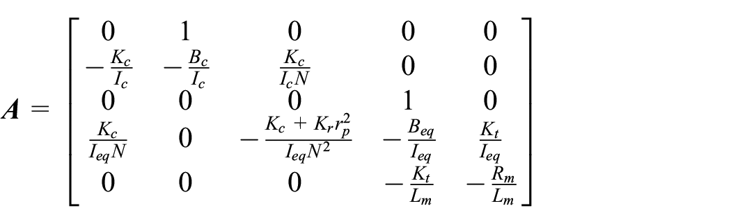
The system is rewritten as a matrix (26).

\frac{\partial}{\partial t} [\underline{x}] = A [\underline{x}] + B \underline{u} (t) + C T_{d} + D T_{r}

(26)

where

A = [\begin{matrix} 0 & 1 & 0 & 0 & 0 \\ - \frac{K_{c}}{I_{c}} & - \frac{B_{c}}{I_{c}} & \frac{K_{c}}{I_{c} N} & 0 & 0 \\ 0 & 0 & 0 & 1 & 0 \\ \frac{K_{c}}{I_{eq} N} & 0 & - \frac{K_{c} + K_{r} r_{p}^{2}}{I_{eq} N^{2}} & - \frac{B_{eq}}{I_{eq}} & \frac{K_{t}}{I_{eq}} \\ 0 & 0 & 0 & - \frac{K_{t}}{L_{m}} & - \frac{R_{m}}{L_{m}} \end{matrix}]

B = {[\begin{matrix} 0 & 0 & 0 & 0 & \frac{1}{L_{m}} \end{matrix}]}^{T}

C = {[\begin{matrix} 0 & \frac{1}{I_{c}} & 0 & 0 & 0 \end{matrix}]}^{T}

D = {[\begin{matrix} 0 & 0 & 0 & - \frac{1}{I_{eq} N} & 0 \end{matrix}]}^{T}

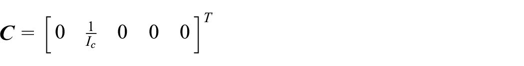
The errors between the output signals ( x ) and the desired signals ( x _des ) are denoted as e (t), according to (27).

\underline{e} (t) = \underline{x} - {\underline{x}}_{des}

(27)

The objective function (cost function) is illustrated by (28).

Q = \frac{1}{2} \int_{0}^{\infty} ({\underline{e}}^{T} (t) E \underline{e} (t) + {\underline{u}}^{T} (t) F \underline{u} (t)) dt

(28)

where E and F are two symmetric matrices such that E is positive semi-definite and F is positive definite. The control signal u (t) is selected according to (29) so that w (t) = 0.

\underline{u} (t) = \underline{w} (t) - R \underline{e} (t)

(29)

Combining (28) and (29), we get (30).

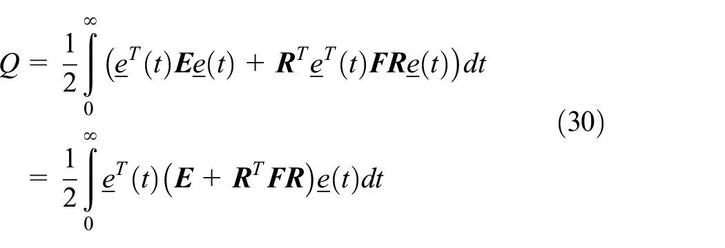
\begin{matrix} Q = \frac{1}{2} \int_{0}^{\infty} ({\underline{e}}^{T} (t) E \underline{e} (t) + R^{T} {\underline{e}}^{T} (t) FR \underline{e} (t)) dt \\ = \frac{1}{2} \int_{0}^{\infty} {\underline{e}}^{T} (t) (E + R^{T} FR) \underline{e} (t) dt \end{matrix}

(30)

The problem’s objective is to minimize the cost function Q. Therefore, finding a control matrix R is necessary to satisfy this target. Matrix R is the equation solution (31), where P is an intermediate matrix. The matrix P is determined by the Riccati algebraic equation, which is presented in equation (32).

FR - B^{T} P = 0

(31)

PB F^{- 1} B^{T} P - PA - A^{T} P = E

(32)

Although the system is linearized, its inputs are nonlinear. Therefore, the traditional LQR algorithm cannot wholly eliminate the system error. To solve this issue, a fuzzy algorithm is proposed to adjust the values of the state variables. The fuzzy algorithm (soft computing) can flexibly adjust the output values based on the changes in the input states and quickly adapt to various operating conditions. The signals of steering column angle (x₁) and steering motor angle (x₃) are adjusted according to (33) and (34), respectively, where x_{1_adj} and x_{3_adj} are the adjustment signals (outputs of fuzzy controllers).

x_{1_new} = x_{1} - x_{1_adj}

(33)

x_{3_new} = x_{3} - x_{3_adj}

(34)

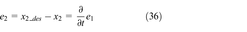
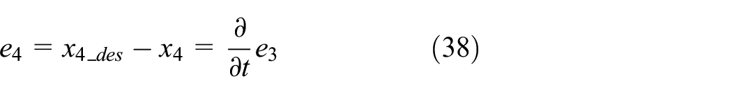
Two fuzzy controllers are designed to apply to two different objects. The first controller has two inputs: Steering Column Angle (SCA) error (e₁) and Steering Column Rate (SCR) error (e₂). Similarly, the second controller’s inputs are Steering Motor Angle (SMA) error (e₃) and Steering Motor Rate (SMR) error (e₄). These errors are illustrated by equations from (35) to (38), where x_des are the desired values determined from the ideal model (Figure 2). Ideal assisted torque (T_{a_ideal}) is looked up from the assisted torque map (Figure 3).

e_{1} = x_{1_des} - x_{1}

(35)

e_{2} = x_{2_des} - x_{2} = \frac{\partial}{\partial t} e_{1}

(36)

e_{3} = x_{3_des} - x_{3}

(37)

e_{4} = x_{4_des} - x_{4} = \frac{\partial}{\partial t} e_{3}

(38)

Figure 2.

Control system diagram.

Figure 3.

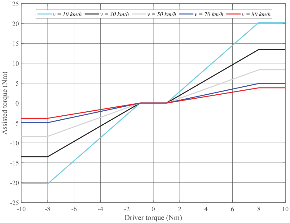
Assisted torque map.

Figure 4 provides information about the membership functions used to design the fuzzy controllers. The first input of the fuzzy controller is formed based on the triangular and trapezoidal functions. Different from the first input, the second input is set by Gaussian functions. The mathematical description of the triangular and trapezoidal functions is expressed by (39) and (40), respectively, while the Gaussian function structure is illustrated by (41), where a, b, c, d, and σ are the coefficients of the membership functions.

f (e_{i}; a, b, c) = max (min (\frac{e_{i} - a}{b - a}, \frac{c - e_{i}}{c - b}), 0)

(39)

f (e_{i}; a, b, c, d) = max (min (\frac{e_{i} - a}{b - a}, 1, \frac{d - e_{i}}{d - c}), 0)

(40)

f (e_{i}, σ, c) = e^{- \frac{{(e_{i} - c)}^{2}}{2 σ^{2}}}

(41)

Figure 4.

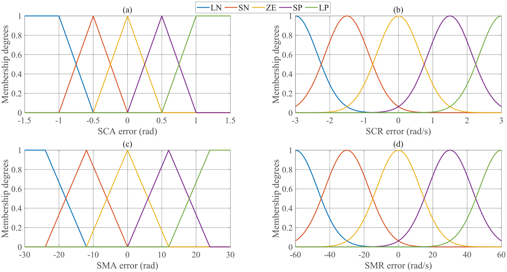
Membership functions: (a) first input (e₁) for steering column, (b) second input (e₂) for steering column, (c) first input (e₃) for steering motor, and (d) second input (e₄) for steering motor.

The triangular function provides a rapid response within a stable range. Once the error exceeds this range, the membership degree must reach saturation. Therefore, the trapezoidal function is used for this purpose. The increase in the value of the Gaussian function is smaller than that of the triangular function, so it helps to avoid overshoot. The membership functions are formed based on the following perspectives:

+ Membership functions need to consider the influence of angle and rate errors instead of just one factor.

+ The variation range of rate error is more extensive than angle error.

+ The steering column angle (x₁) and steering motor angle (x₃) changes must be controlled more closely than other state variables. A small change in the value of x₁ or x₃ can significantly affect the remaining state variables. As a result, we propose using triangular functions to control the changes in these state variables in the stable region. Once the error is significant, the membership degree’s value will reach its maximum. So, the trapezoidal function is used as a saturation limit.

+ The sensitivity of the steering column rate (x₂) and steering motor rate (x₄) is exceptionally high. Therefore, avoiding using functions with steep slopes (such as triangular functions) is necessary. Gaussian functions are a suitable choice for solving this problem.

The output of fuzzy controllers is determined according to fuzzy rules described in Table 1 (steering column) and Table 2 (steering motor), where LN is large negative, SN is small negative, ZE is zero, SP is small positive, and LP is large positive.

Table 1.

Fuzzy rules (steering column).

First input	Second input	Output	First input	Second input	Output
LN	LN	LN	ZE	SP	ZE
LN	SN	SN	ZE	LP	SP
LN	ZE	SN	SP	LN	ZE
LN	SP	ZE	SP	SN	ZE
LN	LP	ZE	SP	ZE	ZE
SN	LN	SN	SP	SP	SP
SN	SN	SN	SP	LP	SP
SN	ZE	ZE	LP	LN	ZE
SN	SP	ZE	LP	SN	ZE
SN	LP	ZE	LP	ZE	SP
ZE	LN	SN	LP	SP	SP
ZE	SN	ZE	LP	LP	LP
ZE	ZE	ZE

Table 2.

Fuzzy rules (steering motor).

First input	Second input	Output	First input	Second input	Output
LN	LN	LN	ZE	SP	SP
LN	SN	LN	ZE	LP	SP
LN	ZE	SN	SP	LN	SN
LN	SP	SN	SP	SN	ZE
LN	LP	ZE	SP	ZE	SP
SN	LN	LN	SP	SP	SP
SN	SN	SN	SP	LP	LP
SN	ZE	SN	LP	LN	ZE
SN	SP	ZE	LP	SN	SP
SN	LP	SP	LP	ZE	SP
ZE	LN	SN	LP	SP	LP
ZE	SN	SN	LP	LP	LP
ZE	ZE	ZE

The 3D graphs in Figure 5 illustrate the above fuzzy rules.

Figure 5.

Fuzzy surfaces: (a) steering column and (b) steering motor.

Simulation and result

Simulation information

In this work, numerical simulations are performed to evaluate the quality of the proposed algorithm. The simulation parameters are listed in Table 3 below.

Table 3.

Specifications.

Symbol	Unit	Value	Symbol	Unit	Value	Symbol	Unit	Value
I _ψ	kgm²	3490	K _c	Nm/rad	126	K _t	Nm/A	0.058
I _c	kgm²	0.06	M _r	kg	31.5	C _αi	N/rad	43,500
I _m	kgm²	0.0004	r _p	m	0.007	l _i	m	1.11/1.69
B _c	Nms/rad	0.065	R _m	Ω	0.41	γ _k	°	10
B _m	Nms/rad	0.0044	L _m	H	0.007	γ _c	°	5
B _r	Ns/m	3630	l _c	m	0.032	m	kg	1650
N	–	17	l _n	m	0.31	K _r	N/mrad	40,000

The quality of the control algorithm is evaluated based on the tracking ability of the output signals, which are illustrated by subplots, including SCA, SCR, SMA, SMR, motor current, and assisted torque. These results are achieved under different input conditions, that is, vehicle speed and driver torque changes. Two types of driver torque are used in this work: J-turn steering (the first case) and sine wave steering (the second case), which are depicted in Figure 6(a). Although sine wave steering is commonly used in theoretical simulations for steering systems, J-turn steering and fish-hook steering are the prevailing choices in practical applications. Specifically, J-turn steering is employed when the vehicle traverses a curve, resulting in an almost circular trajectory. When steering at high speeds, fish-hook steering poses more significant risks than J-turn steering, necessitating the consideration of the vehicle roll angle. In this study, only two types of steering angles, as depicted in Figure 6(a), are utilized. The consideration of fish-hook steering should be reserved for cases where a spatial dynamic model incorporating the rollover condition is applied. The shape of the driver torque signal significantly impacts the output state variables, such as steering column angle, steering motor angle, and others. Therefore, it is necessary to investigate two different types of driver torque signals to determine the performance of the proposed controller instead of just using similar signals.

Figure 6.

Simulation inputs: (a) driver torque and (b) road disturbances (T_rd).

Road disturbances are considered during the simulation according to the description in Figure 6(b). Road disturbances (T_r) are the effects caused by road conditions (such as road surface roughness). A white noise source generates these disturbances and varies randomly over time. In this work, T_r is considered the external disturbance affecting the steering resistance torque (T_sr).

It is necessary to investigate the changes in output variables at different speeds. This purpose uses two speed values: v₁ = 20 km/h and v₂ = 80 km/h. The simulation results are compared under different scenarios: (1) The EPS system is controlled by the linear quadratic tracking control (LQT) algorithm; (2) The EPS system is controlled by the superior algorithm combining fuzzy and linear quadratic tracking control (FLQT); (3) The EPS system is controlled by the PID technique with optimally calculated parameters (PID-GA).

Simulation result

Simulation results are shown in two cases, corresponding to the two types of driver torques illustrated in Figure 6(a).

J-turn steering

J-turn steering is a type of steering commonly used in practice. The value of driver torque increases linearly to its peak and then remains unchanged. In this case, the vehicle’s trajectory is J-shaped.

v ₁ = 20 km/h

The output results obtained from the J-turn steering case are illustrated in Figures 7 and 8. Figure 7 represents the speed v₁ = 20 km/h, while Figure 8 includes the speed v₂ = 80 km/h results.

Figure 7.

Simulation results (J-turn, v₁ = 20 km/h): (a) steering column angle, (b) steering column rate, (c) steering motor angle, (d) steering motor rate, (e) motor current, and (f) driver and assisted torque.

Figure 8.

Simulation results (J-turn, v₂ = 80 km/h): (a) steering column angle, (b) steering column rate, (c) steering motor angle, (d) steering motor rate, (e) motor current, and (f) driver and assisted torque.

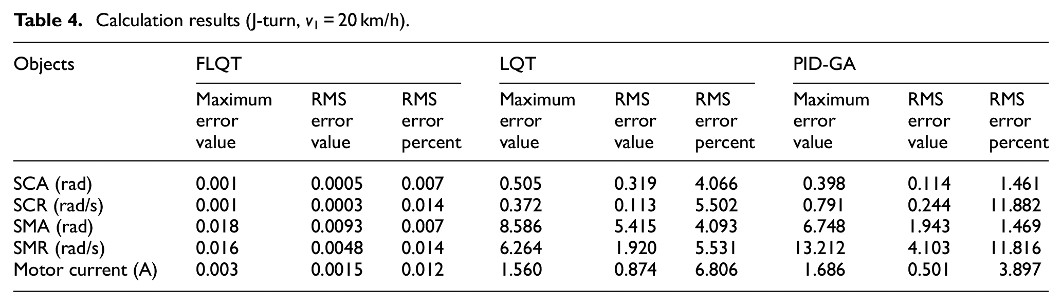
Figure 7(a) shows that the SCA values obtained from the three scenarios all tend to follow the expected value. According to this description, the SCA curve of the LQT scenario is lower than the other two scenarios, indicating that the LQT controller’s error is more significant. The simulation results show that the maximum LQT error is 0.505 rad, and the RMS error is 0.319 rad. Compared to LQT, the PID-GA controller’s error is lower, at only about 0.398 rad (peak value) and 0.114 rad (RMS value). A slight improvement is seen in the FLQT controller, which is proposed in this work. Accordingly, the peak error of SCA is only 0.001 rad, while the RMS error is approximately 0.0005 rad (some results have been rounded). However, the difference between these values is slight. Under the influence of road disturbances, the SCR signal fluctuates slightly instead of being a smooth curve, as depicted in Figure 7(b). Although the SCR signals obtained from the three controllers all follow the value expected, errors between the results still exist. According to the calculation results, PID-GA has the most significant RMS error at 11.882%, while LQT’s error is about half (5.502%). An ideal value is specified by the FLQT controller, which provides stable tracking with an RMS error of only about 0.014%.

Figure 7(c) describes the change of SMA over time when driving in J-turn style at speed v₁ = 20 km/h. The peak error of SMA is 8.586 and 6.748 rad when the EPS system is controlled by LQT and PID-GA techniques, respectively. Regarding RMS error, these values are 5.415 and 1.943 rad, respectively. When replacing the above two controllers with the FLQT controller proposed in this work, the system error is reduced to 0.018 rad (peak value) and 0.0093 rad (RMS value). The performance of the FLQT controller is guaranteed even when the system is subject to road disturbances. As a result (Figure 7(d)), the RMS error of SMR (x₄) is only 0.014% (FLQT), while the figures for the other two scenarios are much more significant: 5.531% (LQT) and 11.816% (PID-GA).

When the vehicle steers at low speed, the power steering efficiency is high, so the motor current signals obtained in this condition tend to follow the desired signal with negligible error. In this condition, the motor current value obtained from the LQT scenario is smaller than the desired value, with an RMS error of 6.806% (Figure 7(e)). This causes the electric motor not to provide enough assisted torque for the EPS system. On the contrary, the motor current value obtained from the PID-GA controller is larger than the reference value with an RMS error of 3.897%, causing a slight excess of assisted torque to be generated. Compared to the above two scenarios, the motor current obtained from the FLQT controller closely follows the desired value with a tiny error (0.012%).

In general, assisted torque increases linearly with driver torque, and assisted torque reaches saturation when driver torque exceeds its limit value (Figure 7(f)). The values obtained from the simulation under v₁ conditions are listed in Table 4 (these values have been rounded). The difference between these values is relatively small, so they can not reflect the controller’s quality proposed in this work. Investigating changes in state variables under different conditions (such as vehicle speed and driver torque changes) is necessary.

Table 4.

Calculation results (J-turn, v₁ = 20 km/h).

Objects	FLQT			LQT			PID-GA
	Maximum error value	RMS error value	RMS error percent	Maximum error value	RMS error value	RMS error percent	Maximum error value	RMS error value	RMS error percent
SCA (rad)	0.001	0.0005	0.007	0.505	0.319	4.066	0.398	0.114	1.461
SCR (rad/s)	0.001	0.0003	0.014	0.372	0.113	5.502	0.791	0.244	11.882
SMA (rad)	0.018	0.0093	0.007	8.586	5.415	4.093	6.748	1.943	1.469
SMR (rad/s)	0.016	0.0048	0.014	6.264	1.920	5.531	13.212	4.103	11.816
Motor current (A)	0.003	0.0015	0.012	1.560	0.874	6.806	1.686	0.501	3.897

v ₂ = 80 km/h

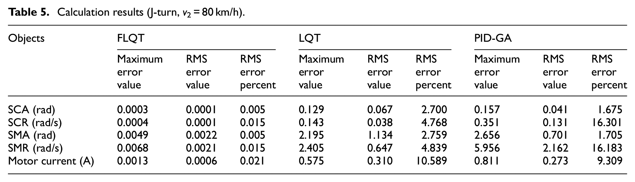
According to the description in Figure 3, the system’s assisted performance will decrease (assisted torque will decrease) as speed increases. Therefore, it is necessary to investigate the changes in state variables at high speed. The output values decrease when the speed increases from v₁ = 20 km/h to v₂ = 80 km/h (Figure 8). The simulation results show that the RMS error of the first state variable (SCA) is 2.700% and 1.675% when the system is controlled by LQT and PID-GA techniques, respectively (Figure 8(a)). Compared to the two results mentioned above, the RMS error belonging to the FLQT controller is tiny, only about 0.005%. The SCR signal is strongly affected by road disturbances (Figure 8(b)). Under the control of the FLQT controller established in this article, the RMS error is maintained within 0.015%, much lower than conventional LQT (4.768%) and PID-GA (16.301%).

The changing trend of SMA is similar to that of SCA, although the value of SMA is much larger than that of SCA (Figure 8(c)). The error of SMA obtained from three controllers is similar to that of SCA. The slightest error still belongs to the FLQT scenario (0.005%). This is true for the fourth state variable (Figure 8(d)).

In this condition, the motor current value is relatively small, which is consistent with the requirements of the initially proposed algorithm (Figure 3). Under the influence of road disturbances, the motor current signal obtained from the PID-GA controller vibrates strongly, increasing maximum error (0.811 A) and RMS error (9.309%). Compared to PID-GA, the motor current value obtained from LQT is smaller, with an RMS error of 10.589%. A significant improvement is seen in the results of the FLQT controller, as its RMS error is only 0.021% (Figure 8(e)). Generally, the results obtained from the proposed algorithm (FLQT) closely follow the reference value with negligible errors. The data obtained from the simulation when steering at speed v₂ is listed in Table 5.

Table 5.

Calculation results (J-turn, v₂ = 80 km/h).

Objects	FLQT			LQT			PID-GA
	Maximum error value	RMS error value	RMS error percent	Maximum errorvalue	RMS error value	RMS error percent	Maximum error value	RMS error value	RMS error percent
SCA (rad)	0.0003	0.0001	0.005	0.129	0.067	2.700	0.157	0.041	1.675
SCR (rad/s)	0.0004	0.0001	0.015	0.143	0.038	4.768	0.351	0.131	16.301
SMA (rad)	0.0049	0.0022	0.005	2.195	1.134	2.759	2.656	0.701	1.705
SMR (rad/s)	0.0068	0.0021	0.015	2.405	0.647	4.839	5.956	2.162	16.183
Motor current (A)	0.0013	0.0006	0.021	0.575	0.310	10.589	0.811	0.273	9.309

The simulation results show that each state variable is small at high speeds. This is due to the degradation in power assist performance, consistent with the assisted torque map proposed in Figure 3. This is designed to enhance the driver’s steering experience at high speeds, necessitating a higher torque output from users. This can improve vehicle stability and reduce the risk of rolling over. The assisted motor will be disconnected once the speed increases too high (90 km/h or more).

The first case only refers to the J-turn steering type. In the following case, we perform simulations with a type of driver torque that continuously varies over time to evaluate the adaptation and response of the proposed algorithm.

Sine wave steering

A sinusoidal form of steering is used in this case (Figure 6). The simulation results are illustrated by subplots in Figures 9 and 10.

Figure 9.

Simulation results (Sine wave, v₁ = 20 km/h): (a) steering column angle, (b) steering column rate, (c) steering motor angle, (d) steering motor rate, (e) motor current, and (f) driver and assisted torque.

Figure 10.

Simulation results (Sine wave, v₂ = 80 km/h): (a) steering column angle, (b) steering column rate, (c) steering motor angle, (d) Steering motor rate, (e) motor current, and (f) driver and assisted torque.

v ₁ = 20 km/h

The change of state variables when steering at speed v₁ = 20 km/h is depicted in Figure 9. The first state variable (SCA) tends to change according to the rules of the input signal. Their maximum errors are 0.556, 1.166, and 0.002 rad, corresponding to the LQT, PID-GA, and FLQT scenarios. The RMS error of the SCA value is 7.214%, 16.705%, and 0.021%, respectively (Figure 9(a)). Regarding SCR, the RMS error can be up to 17.419% when applying the PID-GA technique to the EPS system, while this value is only 0.023% for the FLQT scenario (Figure 9(b)).

When applying the FLQT technique to the EPS system, the RMS error of SMA is only 0.021%, while the error of LQT and PID-GA can be up to 7.250% and 16.777%, respectively (Figure 9(c)). The results obtained for SMR are similar to those obtained for those obtained for SMA (Figure 9(d)). The error is almost completely suppressed when applying the FLQT technique proposed in this work. The FLQT controller’s power consumption is guaranteed to be ideal, with an RMS error of no more than 0.035%. In this case, the motor current value obtained from the PID-GA scenario is much larger than the desired value, with an RMS error of up to 27.386% (Figure 9(e)). This causes the system’s energy consumption to increase.

Figure 9(f) describes the relationship between assisted torque and driver torque. According to this description, the assisted torque obtained from the FLQT controller closely follows the reference value with negligible error. The PID-GA scenario’s systematic error is much greater than that of FLQT and LQT. The simulation results in this scenario are listed in Table 6.

Table 6.

Calculation results (Sine wave, v₁ = 20 km/h).

Objects	FLQT			LQT			PID-GA
	Maximum error value	RMS error value	RMS error percent	Maximum error value	RMS error value	RMS error percent	Maximum error value	RMS error value	RMS error percent
SCA (rad)	0.002	0.001	0.021	0.556	0.355	7.214	1.166	0.823	16.705
SCR (rad/s)	0.004	0.002	0.023	1.112	0.721	7.461	2.815	1.684	17.419
SMA (rad)	0.028	0.018	0.021	9.433	6.028	7.250	19.780	13.950	16.777
SMR (rad/s)	0.061	0.038	0.023	18.833	12.238	7.504	47.907	28.431	17.434
Motor current (A)	0.007	0.004	0.035	2.142	1.337	11.146	6.196	3.285	27.386

v ₂ = 80 km/h

System performance degrades as vehicle speed increases, which is validated in Figure 10. The state variables’ values decrease sharply compared to condition v₁, causing the systematic error to decrease. The results in Table 7 show that the RMS error of the state variables (x₁, x₂, x₃, and x₄) is only about 0.017%. These results are achieved when the system is controlled by the FLQT algorithm proposed in this work. However, the error value increases to nearly 6% and 14% when applying LQT and PID-GA techniques to the EPS system.

Table 7.

Calculation results (Sine wave, v₂ = 80 km/h).

Objects	FLQT			LQT			PID-GA
	Maximum error value	RMS error value	RMS error percent	Maximum error value	RMS error value	RMS error percent	Maximum error value	RMS error value	RMS error percent
SCA (rad)	0.0006	0.0004	0.017	0.221	0.130	5.717	0.474	0.307	13.461
SCR (rad/s)	0.0013	0.0008	0.017	0.435	0.284	5.824	1.133	0.620	12.704
SMA (rad)	0.0108	0.0067	0.018	3.745	2.209	5.818	8.009	5.199	13.689
SMR (rad/s)	0.0224	0.0139	0.017	7.354	4.823	5.928	19.026	10.487	12.892
Motor current (A)	0.0027	0.0016	0.057	0.872	0.521	18.809	2.439	1.178	42.543

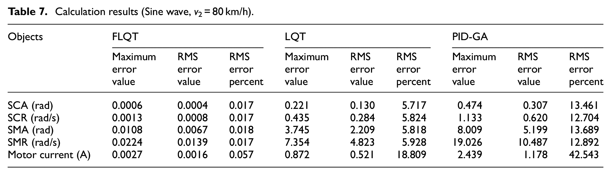
Under the influence of road disturbances, the PID-GA controller’s power consumption increases strongly, 42.543% greater than the desired value. On the contrary, the LQT controller’s motor current value is relatively small, so it cannot meet the initial requirements. The FLQT controller provides robust system control stability with an error of only about 0.057%, much smaller than the other two controllers. As a result, the value of assisted torque obtained from FLQT always closely tracks the desired value with negligible error.

The results obtained from the simulation show:

+ System performance decreases when vehicle speed increases, and vice versa.

+ System performance increases when driver torque increases, and vice versa.

+ In general, the RMS error of the PID-GA scenario is larger than the LQT scenario. Compared to the two scenarios mentioned above, the systematic error obtained from the FLQT scenario is tiny. The values of state variables tend to follow the reference value with negligible error if and only if the system is controlled by the FLQT technique proposed in this work.

+ The PID-GA technique is strongly affected by road disturbances. This is solved by replacing PID-GA with FLQT. Additionally, the power consumption of the proposed controller is significantly improved compared to PID-GA.

+ Once the fuzzy algorithm is integrated with the LQT technique to become FLQT, the algorithm’s performance will be enormously improved. This is demonstrated under simulation conditions.

The results achieved by the FLQT algorithm closely match the ideal values with high accuracy. However, it is essential to note that these results are derived from numerical simulations conducted under ideal operating conditions. This involved linearizing the steering system model, disregarding uncertainties, linearizing the vehicle dynamics model while assuming linear tire deformations, eliminating the influence of external impacts and sensor noise, and addressing other similar factors. Actual output results may vary slightly from simulation results.

Conclusion

Vehicle safety and comfort are ensured by using the EPS system. The control algorithm for the MIMO system is designed in this work based on the combination of the fuzzy algorithm and the linear quadratic tracking control technique called FLQT. The performance of the proposed algorithm is evaluated based on simulation results. According to research findings, the output signals closely follow the reference signal with minimal errors. These results are achieved if the system is controlled by the FLQT technique instead of LQT or PID-GA. System adaptation and response are guaranteed under all survey conditions, even when inputs change and the system is subjected to strong road disturbances.

Although the proposed algorithm provides superior performance to traditional control techniques, some limitations still exist in this work. Firstly, the effects of sensor noise and uncertainties have not been mentioned when investigating the system. Secondly, the fuzzy algorithm proposed in this article is fixed instead of being a superior adaptive algorithm. Thirdly, the ideal characteristic curve must be nonlinear (instead of saturated linear) to make the steering smoother. To solve the above problem, some ideas are proposed: Using observers to estimate state variables to eliminate the influence of sensor noise, establishing an adaptive fuzzy algorithm based on optimization of membership functions, and using sigmoid curves to replace the saturated linear curve. These ideas can be implemented in future work. In addition, conducting related experiments is necessary to evaluate the quality of the proposed algorithm.

Footnotes

Handling Editor: Sharmili Pandian

Declaration of conflicting interests

The author declared no potential conflicts of interest with respect to the research, authorship, and/or publication of this article.

Funding

The author received no financial support for the research, authorship, and/or publication of this article.

ORCID iD

Tuan Anh Nguyen

References

Hartono

Cha

H-R

Shin

KJ.

Design of electric power steering system identification and control for autonomous vehicles based on artificial neural network. IEEE Access 2024; 12: 108460–108471.

Luan

Zhao

Wang

Mode switching and consistency control for electric-hydraulic hybrid steering system. Automot Innov 2024; 7: 166–181.

Allous

Mrabet

Zanzouri

Fast fault-tolerant control of electric power steering systems in the presence of actuator fault. Proc IMechE, Part D: J Automobile Engineering 2019; 233: 3088–3097.

Lee

Chang

Multi-parametric model predictive control for autonomous steering using an electric power steering system. Proc IMechE, Part D: J Automobile Engineering 2019; 233: 3391–3402.

Wang

Karimi

HR.

Experimental study on antivibration control of electrical power steering systems. J Appl Math 2014; 2014: 450427.

Ramasamy

An approach for steering wheel angle evaluation without using a true power-on steering angle sensor in electric power steering systems. J Inst Eng (India) Ser B 2023; 104: 563–568.

Khalkhali

Shojaeefard

Dahmardeh

, et al. Optimal design and applicability of electric power steering system for automotive platform. J Cent South Univ 2019; 26: 839–851.

Xiao

Actuator-integrated fault estimation and fault tolerant control for electric power steering system of forklift. Appl Sci 2021; 11: 7236.

Chen

Guo

Research on control strategy of the electric power steering system for all-terrain vehicles based on model predictive current control. Math Probl Eng 2021; 2021: 6642042.

10.

Hassan

Azubir

NAM

Nizam

, et al. Optimal design of Electric Power Assisted Steering System (EPAS) using GA-PID method. Procedia Eng 2012; 41: 614–621.

11.

Hanifah

Toha

Ahmad

, et al. Swarm-intelligence tuned current reduction for power-assisted steering control in electric vehicles. IEEE Trans Ind Electron 2018; 65: 7202–7210.

12.

Dai

Chen

Zong

, et al. Precise compound control of loading force for electric load simulator of electric power steering test bench. Chin J Mech Eng 2022; 35: 8.

13.

Zheng

Wei

Research on electric power steering fuzzy PI control strategy based on phase compensation. Int J Dyn Control 2022; 11: 1867–1879.

14.

Diab

Valmórbida

Pasillas-Lépine

Linear assistance filter design for electric power steering systems with improved delay margin. Int J Control 2024; 97: 1118–1135.

15.

Manca

Circosta

Khan

, et al. Performance assessment of an electric power steering system for driverless formula student vehicles. Actuators 2021; 10: 165.

16.

, et al. Electric power steering nonlinear problem based on proportional–integral–derivative parameter self-tuning of back propagation neural network. Proc IMechE, Part C: J Mechanical Engineering Science 2020; 234: 4725–4736.

17.

Ramos-Fernández

López–Morales

Márquez-Vera

, et al. Neuro-Fuzzy modelling and stable PD controller for angular position in steering systems. Int J Automot Technol 2021; 22: 1495–1503.

18.

Zhao

, et al. A novel dual power-driven electric power steering system for electric commercial vehicles. Adv Mech Eng 2023; 15: 16878132231200314.

19.

Feng

Zhang

, et al. Dual-motor full-weight electric power steering system for commercial vehicle. Int J Automot Technol 2019; 20: 477–486.

20.

Khasawneh

Das

A robust electric power-steering-angle controller for autonomous vehicles with disturbance rejection. Electronics 2022; 11: 1337.

21.

Kim

You

Lee

S-J

, et al. Robust nonlinear torque control using steering wheel torque model for electric power steering system. IEEE Trans Veh Technol 2023; 72: 9555–9560.

22.

Lee

Chang

, et al. Robust steering-assist torque control of electric-power-assisted-steering systems for target steering wheel torque tracking. Mechatronics 2018; 49: 157–167.

23.

Lian

Liu

, et al. Adaptive fuzzy sliding mode control for electric power steering system. J Mech Sci Technol 2017; 31: 2643–2650.

24.

Qiu

, et al. Torque control of electric power steering systems based on improved active disturbance rejection control. Math Probl Eng 2020; 2020: 6509607.

25.

Zheng

Wei

Research on active disturbance rejection control strategy of electric power steering system under extreme working conditions. Meas Control 2024; 57: 90–100.

26.

Nguyen

TA.

Proposing a BSPID control strategy considering external disturbances for electric Power steering (EPS) systems. IEEE Access 2023; 11: 143230–143249.

27.

Nguyen

TA.

Development of a novel integrated control strategy for automotive electric power steering systems. IEEE Trans Autom Sci Eng 2024; 22: 926–943.

28.

Nguyen

Tran

TTH

Nguyen

, et al. Application of MIMO control algorithm for active suspension system: a new model with 5 state variables. Latin Am J Solids Struct 2022; 19: e435.

29.

Chitu

Lackner

Horn

, et al. Controller design for an electric power steering system based on LQR techniques. Compel 2013; 32: 763–775.

30.

Irmer

Henrichfreise

Design of a robust LQG compensator for an electric power steering. IFAC Pap OnLine 2020; 53: 6624–6630.

31.

Mehrabi

McPhee

Azad

NL.

Design and evaluation of an observer-based disturbance rejection controller for electric power steering systems. Proc IMechE, Part D: J Automobile Engineering 2016; 230: 867–884.

32.

Pang

Shang

, et al. Optimal design of fault-tolerant controller for an electric power steering system with sensor failures using genetic algorithm. Shock Vib 2018; 2018: 1801589.

33.

Sorial

Soliman

Hasanien

, et al. A vector controlled drive system for electrically power assisted steering using Hall-Effect sensors. IEEE Access 2021; 9: 116485–116499.

34.

Murilo

Rodrigues

Teixeira

ELS

, et al. Design of a parameterized model predictive control for electric power assisted steering. Control Eng Pract 2019; 90: 331–341.

35.

Jang

Lee

Kim

, et al. Road torque modeling for electric power steering systems. Int J Autom Technol 2022; 23: 765–773.

36.

Nguyen

TA.

Proposing a novel fuzzy control algorithm for automotive active stabilizer bars based on views of roll stability and ride comfort. Proc IMechE, Part K: J Multi-body Dynamics 2023; 237: 585–600.

First input	Second input	Output	First input	Second input	Output
LN	LN	LN	ZE	SP	ZE
LN	SN	SN	ZE	LP	SP
LN	ZE	SN	SP	LN	ZE
LN	SP	ZE	SP	SN	ZE
LN	LP	ZE	SP	ZE	ZE
SN	LN	SN	SP	SP	SP
SN	SN	SN	SP	LP	SP
SN	ZE	ZE	LP	LN	ZE
SN	SP	ZE	LP	SN	ZE
SN	LP	ZE	LP	ZE	SP
ZE	LN	SN	LP	SP	SP
ZE	SN	ZE	LP	LP	LP
ZE	ZE	ZE

First input	Second input	Output	First input	Second input	Output
LN	LN	LN	ZE	SP	SP
LN	SN	LN	ZE	LP	SP
LN	ZE	SN	SP	LN	SN
LN	SP	SN	SP	SN	ZE
LN	LP	ZE	SP	ZE	SP
SN	LN	LN	SP	SP	SP
SN	SN	SN	SP	LP	LP
SN	ZE	SN	LP	LN	ZE
SN	SP	ZE	LP	SN	SP
SN	LP	SP	LP	ZE	SP
ZE	LN	SN	LP	SP	LP
ZE	SN	SN	LP	LP	LP
ZE	ZE	ZE

First input	Second input	Output	First input	Second input	Output
LN	LN	LN	ZE	SP	ZE
LN	SN	SN	ZE	LP	SP
LN	ZE	SN	SP	LN	ZE
LN	SP	ZE	SP	SN	ZE
LN	LP	ZE	SP	ZE	ZE
SN	LN	SN	SP	SP	SP
SN	SN	SN	SP	LP	SP
SN	ZE	ZE	LP	LN	ZE
SN	SP	ZE	LP	SN	ZE
SN	LP	ZE	LP	ZE	SP
ZE	LN	SN	LP	SP	SP
ZE	SN	ZE	LP	LP	LP
ZE	ZE	ZE

First input	Second input	Output	First input	Second input	Output
LN	LN	LN	ZE	SP	SP
LN	SN	LN	ZE	LP	SP
LN	ZE	SN	SP	LN	SN
LN	SP	SN	SP	SN	ZE
LN	LP	ZE	SP	ZE	SP
SN	LN	LN	SP	SP	SP
SN	SN	SN	SP	LP	LP
SN	ZE	SN	LP	LN	ZE
SN	SP	ZE	LP	SN	SP
SN	LP	SP	LP	ZE	SP
ZE	LN	SN	LP	SP	LP
ZE	SN	SN	LP	LP	LP
ZE	ZE	ZE

A linear quadratic tracking control strategy based on fuzzy for electric power steering systems

Abstract

Keywords

Introduction

Mathematical model

C-EPS system model

Fuzzy linear quadratic tracking control

Simulation and result

Simulation information

Simulation result

J-turn steering

v 1 = 20 km/h

v 2 = 80 km/h

Sine wave steering

v 1 = 20 km/h

v 2 = 80 km/h

Conclusion

Footnotes

Declaration of conflicting interests

Funding

ORCID iD

References

v ₁ = 20 km/h

v ₂ = 80 km/h

v ₁ = 20 km/h

v ₂ = 80 km/h

First input	Second input	Output	First input	Second input	Output
LN	LN	LN	ZE	SP	ZE
LN	SN	SN	ZE	LP	SP
LN	ZE	SN	SP	LN	ZE
LN	SP	ZE	SP	SN	ZE
LN	LP	ZE	SP	ZE	ZE
SN	LN	SN	SP	SP	SP
SN	SN	SN	SP	LP	SP
SN	ZE	ZE	LP	LN	ZE
SN	SP	ZE	LP	SN	ZE
SN	LP	ZE	LP	ZE	SP
ZE	LN	SN	LP	SP	SP
ZE	SN	ZE	LP	LP	LP
ZE	ZE	ZE

First input	Second input	Output	First input	Second input	Output
LN	LN	LN	ZE	SP	SP
LN	SN	LN	ZE	LP	SP
LN	ZE	SN	SP	LN	SN
LN	SP	SN	SP	SN	ZE
LN	LP	ZE	SP	ZE	SP
SN	LN	LN	SP	SP	SP
SN	SN	SN	SP	LP	LP
SN	ZE	SN	LP	LN	ZE
SN	SP	ZE	LP	SN	SP
SN	LP	SP	LP	ZE	SP
ZE	LN	SN	LP	SP	LP
ZE	SN	SN	LP	LP	LP
ZE	ZE	ZE