Research on robot obstacle avoidance algorithm based on convolutional neural network

Abstract

Traditional obstacle avoidance algorithms usually use a single shallow application, such as sensor-based distance measurement or some logic judgment algorithm, which leads to problems such as the need to manually adjust the parameters first, the inability to recognize complex or unknown environments, and the recognition errors caused by significant noise errors. Therefore, to overcome these limitations, this paper combines convolutional neural network and obstacle avoidance algorithms. A model of obstacle avoidance method based on convolutional neural network established in this paper, and puts forward the theory of obstacle avoidance method based on convolutional neural network, which adopts MobileNet_v3 as the learning framework, roughly classifies all the obstacle maps into three categories, and then, through the research and application of six traditional obstacle avoidance algorithms, finally concludes that the model can be applied according to different kinds of obstacles. The model can learn and discriminate against different obstacle maps, thus improving the performance of obstacle avoidance and avoiding the limitations of traditional obstacle avoidance algorithms. Verified the effectiveness of each algorithm in various scenarios. A single shallow application of the problem is usually used to robotize the traditional obstacle avoidance algorithms, which provides an essential reference.

Introduction

Path planning is finding the best path from a starting point to an endpoint or the path that optimizes some objective function in a given environment. This process usually needs to consider the limitations of the environment and constraints, such as obstacles, terrain, etc., and the depreciation of specific metrics, such as time, distance, and cost. Path planning is the basis of many real-world problems, such as robot navigation, ¹ driverless cars, ² and circuit board wiring. Most traditional path-planning algorithms are based on classical algorithms such as graph search, heuristic search, dynamic programming, etc. Although they can get good results in many scenarios, their performance in complex environments tends to be greatly limited; for example, when facing the presence of a large number of obstacles in the environment, complex road conditions, or the presence of multiple targets, traditional path planning algorithms do not perform well.

In recent years, the development of deep learning technology has brought new opportunities to path planning. As a powerful machine learning method, deep learning is characterized by high adaptivity, good generalization performance, scalability, etc. It can automatically extract features and generate high-quality decision models by learning a large amount of data. These advantages are well-suited for path-planning problems.^3–5

Among them are two main categories of deep learning convolutional neural network-based robot trajectory planning methods: image-based path planning^6–11 and sensor data-based path planning.^12–14 Deep learning convolutional neural networks are essential to image- and sensor-data-based path planning. The algorithmic model can effectively solve the path-planning problem in complex situations and provides new ideas and methods for the further development of path-planning algorithms.

The mobile robot environment model discussed in this paper refers to a spatial environment model that helps to solve the robot’s path planning problem. Free space is a work area in which an autonomous robot can move freely in that environment. Therefore, the following assumptions need to be made in this paper to facilitate free space modeling.

• (1) The spatial environment of the robot is two-dimensional.

• (2) The spatial environment and obstacles are static, the space is rectangular, and the obstacles are all defined as circles. In this paper, the number and density of obstacles will be varied to simulate three robot working conditions.

• (3) To ensure a safe distance between the planned path and all obstacles, the obstacle boundary is extended outward as a virtual obstacle, and its size is based on the minimum cross-section of the robot as well as the minimum detection distance of the sensors.

• (4) In this paper, the robot has a non-negligible radius, increasing its credibility in practical scenarios.

In this paper, a new hybrid model is proposed with the aid of this new idea, which uses convolutional neural networks to label various types of obstacle maps and is tested using various classical algorithms to derive the adaptability of the respective algorithms to different obstacle maps, respectively, as a way to optimize the obstacle avoidance choices of mobile robots. Firstly, various types of obstacle maps are generated to label and classify a dataset using Mobilenet_v3. The Dijkstra, A*, PRM, RRT, RRT*, and Informed RRT* algorithms are utilized to seek suboptimal trajectory lengths of collision-free obstacles, and finally, the relevant conclusions are drawn.

Introduction to the adopted algorithm

Introduction to the selected convolutional neural network

A convolutional neural network (CNN) class of classical deep learning models for raster data such as images and videos. It specializes in processing data with grid-like structures such as images, videos, etc. CNNs can automatically extract features from these data and be used for classification, target detection, semantic segmentation, etc.^15–17 The neural network algorithm selected in this paper is MobileNet, the newest and superior lightweight convolutional neural network. It has the advantages of high accuracy and low computational effort and meets the research needs of this paper. This convolutional neural network was upgraded to the MobileNet_V3 ¹⁸ version by Andrew G. Howard’s team in 2019.

The core principle of MobileNet is Depthwise Separable Convolution, which operates by splitting the traditional convolution operation into two operations to reduce the computational effort significantly. Specifically, in Depthwise Separable Convolution, the input data is first processed by a Depthwise Convolution layer, which only performs spatial convolution on each input channel separately, called “channel-by-channel convolution.” A Pointwise Convolution layer then combines the output of the depthwise convolution with a single filter to produce the final feature map. This dramatically reduces computation and memory requirements and speeds up the inference process while maintaining relatively high accuracy. MobileNet also introduces Linear Bottlenecks to reduce computation further. It applies a nonlinear activation function ReLU6 (pruning values less than 0 and greater than 6) to the deep convolution output. It feeds it into the point convolution layer for linear combination. This approach reduces the redundant information in the feature map and improves the running speed. Its structure is shown in Figure 1.

Figure 1.

Mobilenet_v3 structure.

In Mobilenet_v3, swish is introduced as an activation function, which can improve accuracy by replacing ReLU in neural networks. However, due to the high computational cost of Swish, ¹⁹ it consumes a lot of resources when used on mobile devices. They propose a novel activation function called h-swish, which has almost the same effect as Swish but with a much lower computational cost. Specifically, h-swish is realized by simplifying the equation of Swish, that is, by using h-swish instead of Swish, the computational burden of the model can be significantly reduced without sacrificing the accuracy, which makes it more suitable for running in restricted environments such as mobile devices. The specific equations are as follows:

$$h-\mathrm{swish}[x]=x\frac{\mathrm{Re}\mathrm{LU}6(x+3)}{6}$$

(1)

To summarize, this article uses the MobileNet_V3 convolutional neural network algorithm improved by previous researchers, which has the advantages of small computing and memory overhead, suitable for mobile devices and embedded system applications, and relatively high accuracy. Specifically, the path planning algorithm can extract information such as roads and obstacles from the scene for target detection or segmentation tasks. Such data can then be fed into a path planning algorithm, such as the A* algorithm or Dijkstra’s algorithm, to calculate the optimal path. Further, the MobileNet_V3 model can be fine-tuned by techniques such as fine-tuning to meet the needs of specific application scenarios.

Six algorithms for proposed comparisons

A* algorithm

The development of the A* algorithm can be traced back to 1968 when Hart, Nilsson, and Raphael19 proposed it and called it the “A* search algorithm.” Later, Nils Nilsson renamed it the A* algorithm and published a more complete description and analysis of the algorithm.

Specifically, the A* algorithm is a heuristic search algorithm that uses heuristic information, the estimated distance to the destination, to guide the search direction and to efficiently search large-scale spaces. The algorithm first needs to initialize the start and end nodes, add the start point to the open list, and set its g-value to 0 and its f-value to h-value (i.e., the start-to-destination estimation function). Then the loop starts traversing the following operations until the endpoint is found or the open list is empty (at this point, there is no solution):

• (1) From the open list, select the node with the smallest f value as the current node and then delete it from the list.

• (2) If the current node is the end point node, return the path.

• (3) Perform the following operations on all neighboring nodes of the current node:

•    b. If the neighbor node is not in the open list, drop it into the open list and update its g and f values.

•    c. If this neighboring node is already in the open list, update its g and f values and reset its parent node.

(4) Add the current node to the closed list.

Where the g value of a node indicates the actual cost from the starting point to that node, and the f value indicates the total cost from the starting point to that node. That is:

$$f(n)=g(n)+h(n)$$

(2)

Where g(n) is the two-node walking cost; h(n) is the heuristic function. Where for the distance cost g(n), there are three calculation methods: Manhattan distance, Euclidean distance, and diagonal distance. Each of the three computational methods has its application: if only four directions are allowed to move in the graph, Manhattan distance is used; if eight directions are allowed to move in the graph, diagonal distance is used; if any direction is allowed to move in the graph, Euclidean distance is used. The moving environment described in this paper provides like movement in any direction, so the Euclidean distance is taken as the calculation method, that is:

$$D=\sqrt{{(x_2-x_1)}^2+{(y_2-y_1)}^2}$$

(3)

Dijkstra’s algorithm

Dijkstra’s algorithm is a classical algorithm representing the shortest path to a single source in a directed graph with entitled values. Its developmental origins can be traced back to the “shortest path problem from the source to each vertex” proposed by the Dutch computer scientist Edsger W. Dijkstra in 1956, ²⁰ whose nature is a particular case of the A* algorithm when h(n) = 0. The pseudo-code is shown in Table 1 below.

Table 1.

Pseudo-code of Dijkstra’s algorithm.

Dijkstra algorithm
1    for each vertex $\upsilon \in G.V$
2               $\upsilon .d\leftarrow \infty$
3               $\mathit{\upsilon }.\mathit{\pi }\leftarrow \mathit{NIL}$
4               $s.d\leftarrow 0$
5               $S\leftarrow \varnothing$
6               $Q\leftarrow G.V$
7    while $Q\ne \varnothing$
8             $\mathit{u}=\mathit{EXRACT}-\mathit{MIN}(\mathit{Q})$
9               $\mathit{S}\leftarrow \mathit{S}\cup \left\{\mathit{u}\right\}$
10  for each vertex $\mathbf{\nu }\in \mathit{G}.\mathit{Adj}\left[\mathit{u}\right]$
11              $\mathit{RELAX}(\mathit{u},\mathbf{\nu },\mathbf{\omega })$
12  end for
13   end while

Probabilistic road map algorithm

The origin of the PRM algorithm can be traced back to 1996 when Lydia Kavraki and Jean-Claude Latombe published an article, “Probabilistic Roadmaps for Path Planning in High-Dimensional Configuration Spaces.” ²¹ In this paper, the PRM algorithm is studied and analyzed. It is a probabilistic sampling-based path planning algorithm that creates a road map (roadmap) by randomly sampling in free space and using this map for path searching. The PRM algorithm has a high success rate and real-time performance and is widely used in robotics, UAVs, and other fields. Its pseudo-code is shown in Table 2 below.

Table 2.

Pseudo code of PRM algorithm.

PRM algorithm
1              $\mathit{V}\leftarrow \varnothing$
2              $E\leftarrow \varnothing$
3     while $\left|\mathit{V}\right|<n$
4    Repeat
5        $q\leftarrow a\mathrm{random}\mathrm{configuration}\mathrm{in}Q$
6    until $q\mathrm{is}\mathrm{collision}-\mathrm{free}$
7             $V\leftarrow V\cup \left\{q\right\}$
8     end while
9     for all $q\in V$ do
10   ${\mathit{N}}_{\mathit{q}}\leftarrow \mathit{t}\mathit{h}\mathit{e}k\mathit{c}\mathit{l}\mathit{o}\mathit{s}\mathit{e}\mathit{s}\mathit{t}\mathit{n}\mathit{e}\mathit{i}\mathit{g}\mathit{h}\mathit{b}\mathit{o}\mathit{r}\mathit{s}\mathit{o}\mathit{f}q\mathit{c}\mathit{h}\mathit{o}\mathit{s}\mathit{e}\mathit{n}\mathit{f}\mathit{r}\mathit{o}\mathit{m}V\mathit{a}\mathit{c}\mathit{c}\mathit{o}\mathit{r}\mathit{d}\mathit{i}\mathit{n}\mathit{g}\mathit{t}\mathit{o}\mathit{d}\mathit{i}\mathit{s}\mathit{t}$
11   for all $\mathit{q}\prime \in {\mathit{N}}_{\mathit{q}}$ do
12    if $(q,q\prime )\notin \mathit{E}$ and $\mathit{\Delta }(q,q\prime )\ne \mathit{NIL}$ then
13            $\mathit{E}\leftarrow \mathit{E}\cup \left\{(q,q\prime )\right\}$
14     end if
15   end for
16    end for

RRT algorithm

The origin of the development of the RRT (Rapidly-exploring Random Trees) algorithm can be traced back to the year 2000, which was proposed by Steven M. LaValle. ²² The RRT algorithm is a random tree search algorithm used to solve high-dimensional space path planning problems. Its main feature is randomly sampling and quickly generating an exploratory tree during the search process. This algorithm can effectively cope with high-dimensional space and complex obstacle scenes and has performed well in practical applications.

To facilitate the understanding of the principle of the RRT algorithm and its improved algorithms, firstly, the relevant function definitions in this algorithm are explained for the following:

Sample function: generates sample points x_sample using a certain number of random numbers in the space where path planning is performed.

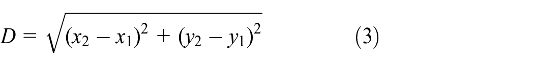
Nearest function: the nearest node function, defined as selecting a node x in a random tree T and using a specific metric function ρ such that it simultaneously satisfies x∈T and point x is the nearest point x_nearest of x_sample. The general metric function uses the Euclidean distance as shown in equation (4):

$$\rho (x_1,x_2)=\Vert x_2-x_1\Vert$$

(4)

Steer function: this function is used to generate a new node step is: for a given step, by random sampling to get the sampling points x_nearest, and according to the nearest node Nearest function, calculate the nearest node x_nearest. Then, a new node can be generated from equation (5) such that x_new, and x_new∈T. A node x_new is a node that starts at the node x_nearest. The new node is obtained by moving in a direction.

$$\begin{array}{c}{x}_{\mathrm{new}}\leftarrow \mathrm{Steer}(x_{\mathrm{nearest}},x_{\mathrm{sample}}):\hfill \\ \{x_{\mathrm{new}}:x_{\mathrm{new}}=x_{\mathrm{nearest}}+\mathrm{step}\times \frac{x_{\mathrm{sample}}-x_{\mathrm{nearest}}}{\parallel x_{\mathrm{sample}}-x_{\mathrm{nearest}}\parallel }\}\hfill \end{array}$$

(5)

The RRT* algorithm

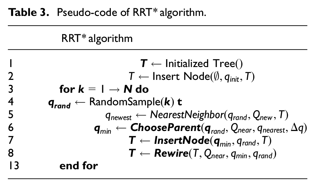
The origin of the development of the RRT* (Rapidly-exploring Random Tress Star) algorithm can be traced back to 2005, proposed by LaValle and Kuffner. ²³ The RRT* algorithm is an improved and upgraded algorithm that is designed to solve the path planning problem in high dimensional spaces. The algorithm can better explore the feasible path space and find the global optimal solution by introducing optimization strategies and reconnection techniques. Its pseudo-code is shown in Table 3 below.

Table 3.

Pseudo-code of RRT* algorithm.

RRT* algorithm
1            $\mathit{T}\leftarrow \mathrm{Initialized}\mathrm{Tree}()$
2           $T\leftarrow \mathrm{Insert}\mathrm{Node}(\varnothing ,q_{\mathrm{init}},T)$
3    for $\mathit{k}=1\to \mathit{N}$ do
4    ${\mathit{q}}_{\mathit{rand}}\leftarrow \mathrm{RandomSample}(\mathit{k})$ t
5         $q_{\mathrm{newest}}\leftarrow \mathrm{NearestNeighbor}(q_{\mathrm{rand}},Q_{\mathrm{new}},T)$
6        ${\mathit{q}}_{\min }\leftarrow \mathit{ChooseParent}({\mathit{q}}_{\mathrm{rand}},Q_{\mathrm{near}},q_{\mathrm{nearest}},\mathrm{\Delta }q)$
7           $\mathit{T}\leftarrow \mathit{InsertNode}({\mathit{q}}_{\min },q_{\mathrm{rand}},T)$
8           $\mathit{T}\leftarrow \mathit{Re}\mathit{wire}(T,Q_{\mathrm{near}},q_{\min },q_{\mathrm{rand}})$
13    end for

The informed RRT* algorithm

The origin of the Informed RRT* algorithm can be traced back to 2006, when it was first proposed by Sertac Karaman and Emilio Frazzoli in their paper. ²⁴ The algorithm is based on RRT* and explores the search space more intelligently by introducing heuristic search techniques. Its pseudo-code is shown in Table 4 below.

Table 4.

Pseudo-code of Informed RRT* algorithm.

Informed RRT* algorithm
1  if ${\mathit{c}}_{\mathit{max}}$ then
2            $c\Vert x_{goal}-x_{start}{\Vert }_{2min}$
3           ${\mathit{x}}_{\mathrm{centre}}\leftarrow ({\mathit{x}}_{\mathrm{start}}+x_{\mathrm{goal}})/2$
4        $\mathrm{cRotationToWorldFrame}{x}_{\mathrm{start}}+{x_{\mathrm{goal}}}_{\min }$
5             $r_1\leftarrow c_{\max }/2$
6          ${\left\{r_i\right\}}_{i=2,...,n}\leftarrow (\sqrt{c_{\max }^2-c_{\min }^2})/2$
7             $L\leftarrow \mathrm{diag}\{r_1,...,r_n\}$
8            ${\mathit{x}}_{\mathit{ball}}\leftarrow \mathrm{SampleUnitBall}$
9           ${\mathit{x}}_{\mathit{rand}}\leftarrow (\mathrm{CL}{\mathit{x}}_{\mathit{ball}}+{\mathit{x}}_{\mathit{centre}})\cap \mathit{X}$
10  Else
11              ${\mathit{x}}_{\mathit{rand}}~\mathit{U}(\mathit{X})$
12  return ${\mathit{x}}_{\mathit{rand}}$

Simulation

Implementation environment and configuration

The model simulation can be carried out after selecting the appropriate neural network convolutional model and formulating the six algorithms for testing. The environment and configuration of this simulation include the configuration of tools and hardware devices such as PyTorch, Python 3.9, VS Code, GPU 1660ti, and some parameters related to the simulation. The roadblock maps are divided into three categories: Sparse, Normal, and Dense. Their size is uniformly 200 mm in length and 170 mm in height, the obstacles are black circles, and the number of obstacles in different types of obstacle maps is significantly different. The robot radius is 2 mm, and the convolutional neural network model is MobileNet_v3.

Implementation scheme and technical route

The specific research route of this simulation is shown in Figure 2 below, and the main steps are as follows.

• (1) Data collection and pre-processing: Create all kinds of maps, obstacles, start and end points, and other information required for path planning, and clean, format, convert, and standardize the data to ensure its availability and quality.

• (2) Convolutional neural network model design and training: Convolutional neural network (Mobile) is used as the deep learning model, and the data is classified by differentiating different path conditions with labels. At the same time, methods such as regularization and optimizer are used to perform training and optimization operations on the model to ensure that the accuracy and robustness of the model are maximized.

• (3) Traditional path planning algorithm implementation: common path planning algorithms (e.g., A* algorithm, Dijkstra’s algorithm, RRT algorithm, etc.) are selected, implemented, and debugged to ensure that the algorithms can plan paths correctly and effectively.

• (4) Algorithm adaptive implementation: embed the trained and debugged deep learning mobilenet_v3 model into the traditional path planning algorithms to choose the most suitable algorithm to plan the path according to the current path conditions, thus achieving better performance.

• (5) Evaluation and analysis of simulation results: by analyzing and comparing the simulation results, the performance and advantages and disadvantages of different algorithms under different obstacle maps can be compared, and improvements and future research directions can be proposed. Similarly, the simulation results can also be compared with other existing algorithms, and their feasibility and application value can be evaluated based on practical application scenarios.

Figure 2.

Research line of robot obstacle avoidance method based on convolutional neural network.

Introduction to the dataset

The dataset was completely self-made by writing code in Python and using Matplotlib to draw a plane 200 mm long and 150 mm high with black solid circles of random radius size but with radius intervals ranging from 8 mm to 24 mm and obstacle images with random locations. Still, the circles do not intersect, and there is a little distance between them.

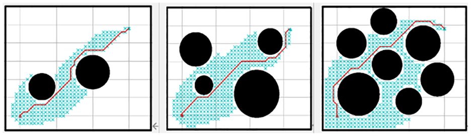
These include sparse, normal, and dense form obstacle images; each category contains 500 training images and 50 validation images, totaling 1500 training images and 150 validation images. No data filtering or preprocessing was performed in this dataset. The dense, balanced, and loose obstacle maps represent different types of images, and the labels of these three categories are defined as “Sparse,”“Normal,” and “Dense.” Regarding statistical features, each image is the same size with 224 pixels, the color is white with black barriers, and the barriers are uniformly rounded to facilitate comparison practice, as in Figure 3.

Figure 3.

Schematic representation of the data set (from left to right: loose, normal, dense).

Simulation analysis of MobileNet_v3

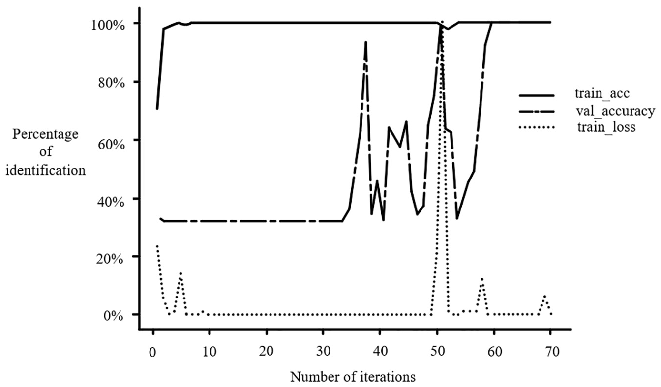
This simulation investigates MobileNet_v3’s performance with deep learning convolutional networks on the image classification task, recognition performance is shown in Figure 4 below. It verifies whether it can accurately classify different obstacle maps to implement the selection operation of different obstacle maps for the path planning algorithm. We will next learn to train the dataset above and conduct a validation simulation simultaneously.

Figure 4.

Recognition performance.

Where the blue line train_loss is the loss function value of the training set, the yellow line train_acc is the classification accuracy of the training set, and the green line val_accuracy is the classification accuracy of the validation set. Each line of data corresponds to a training round, and it can be seen that the number of training rounds goes from 1 to 70, where the highest and most stable accuracy is in round 59 and beyond, with the training set validation set reaching 100%. It can also be seen that during the training process, the accuracy and loss fluctuate, but the overall trend is that the accuracy gradually increases and the loss gradually decreases. This indicates that the model gradually learns a better feature representation during training, improving accuracy.

Simulation analysis of MobileNet_v3

In training the convolutional neural network MobileNet_v3 model, this paper found that the model has high classification accuracy and stability and can accurately classify different obstacle images. This efficient image classification ability provides more possibilities for practical applications and can give quasi-input data for subsequent obstacle avoidance algorithms. Therefore, based on the classification results of the MobileNet_v3 model, we can allow the model to automatically select different obstacle avoidance algorithms to cope with varying images of obstacles with optimal performance and improve the effect and performance of obstacle avoidance. As shown in Table 5, the suboptimal path charts of each algorithm in different types of obstacle maps were obtained through many repeated tests.

Table 5.

The performance of six obstacle avoidance algorithms in three types of obstacle maps.

Types of Algorithms	Sparse	Normal	Dense
A*	Path length = 211.4 Time-consuming = 1.1 s	Path length = 217 Time-onsuming = 1.5 s	Path length = 238.5 Time-consuming = 1.8s
Dijkstra	Path length = 211.4 Time-consuming = 12s	Path length = 217 Time-consuming = 5.9s	Path length = 238 Time-consuming = 3.9s
PRM	Path length = 207 Time-consuming = 4.9 s	Path length = 217.7 Time-consuming = 3.6 s	Path length = 231.4 Time-consuming = 3.8 s
RRT	Path length = 246.9 Time-consuming = 3.7s	Path length = 228 Time-consuming=4.5 s	Path length = 252 Time-consuming=7 s
RRT*	Path length = 201 Time-consuming = 12 s	Path length = 216 Time-consuming=9.7 s	Path length = 220 Time-consuming = 10 s
Informed RRT*	Path length = 204 Time-consuming = 16 s	Path length = 225 Time-consuming = 7.5 s	Path length = 198 Time-consuming = 22 s

Analysis of simulation data

Specific analysis of the A* algorithm’s three types of obstacle maps

The A* algorithm is based on a heuristic search that guides the search direction by estimating the distance from the start point to the endpoint to find the shortest path efficiently. In path planning problems, the A* algorithm usually considers the optimal solution faster than other search algorithms.

Figure 5 shows that the A* algorithm performs well under both loose and normal obstacles, with the optimal path length performance. This is because, in these cases, the A* algorithm can fully utilize the information of heuristic functions to guide the search direction and quickly find the shortest path. However, under dense obstacles, the A* algorithm performs relatively poorly. This is because, in this case, the search space is huge, and the estimation of the heuristic function may be inaccurate, leading the algorithm to fall into a local optimal solution or a situation where no solution can be found. To solve this problem, some optimization strategies can be used, such as increasing the cost of obstacles or using more complex heuristic functions.

Figure 5.

Effectiveness of A* algorithm.

Specific analysis of Dijkstra’s algorithm for three types of obstacle maps

Dijkstra’s algorithm is a classical shortest-path search algorithm that finds the shortest path from the start to the end by traversing all nodes. Unlike the A* algorithm, Dijkstra’s algorithm does not use a heuristic function to guide the search direction, so it needs to consider more nodes, and the search time is relatively longer.

In Figure 6, we can see that Dijkstra’s algorithm’s performance in terms of path length under the three obstacles is comparable to that of the A* algorithm, which is because, in this case, the information from the heuristic function is not very useful in guiding the direction of the search. The Dijkstra algorithm’s strategy of traversing all the nodes can find the shortest path.

Figure 6.

Effectiveness of Dijkstra’s algorithm.

However, in terms of time consumption, Dijkstra’s algorithm lags behind a bit. This is because, in these cases, the search space is huge, Dijkstra’s algorithm needs to traverse more nodes, and the search time is relatively long. In contrast, the A* algorithm can use the information from the heuristic function to guide the direction of the search so that the shortest path can be found quickly.

Specific analysis of the PRM algorithm’s three types of obstacle map

PRM algorithm is a sampling-based path search algorithm that searches for the shortest path by constructing an undirected graph in advance. Unlike A* and Dijkstra algorithms, the PRM algorithm does not need to traverse the whole search space but constructs the undirected graph by sampling some key points, thus reducing the search time.

Figure 7 shows that the PRM algorithm performs relatively moderately well under all three obstacles. This may be because the randomness in its graph construction process consumes little time under different obstacle graphs. The length of the paths it plots is not an optimal solution, but it is not too bad either.

Figure 7.

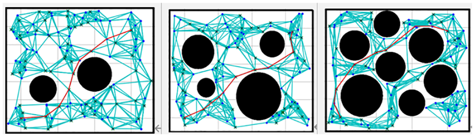
Effectiveness of the PRM algorithm.

Specific analysis of the RRT algorithm for three types of obstacle graphs

The RRT algorithm is an exploration-based algorithm for rapidly generating path trees in geometric space with stochasticity. It explores the space by starting from the starting point and successively adding new nodes to the tree until the endpoint is found. Unlike the A* and Dijkstra algorithms, the RRT algorithm does not require pre-constructed graphs but explores the space by random sampling, making it suitable for problems with complex geometries.

In Figure 8, we can see that the RRT algorithm is not guaranteed to find the optimal solution in the three obstacle graphs mentioned above, and the length of the planned path is the longest in all of them. This is because the exploration process of the RRT algorithm is random and may miss some important paths or fall into local optimal solutions. In addition, the search efficiency of the RRT algorithm is also affected by the number and distribution of sampling points, which may lead to a decrease in the search efficiency if the sampling points are too few or unevenly distributed.

Figure 8.

Effectiveness diagram of the RRT algorithm.

Specific analysis of the RRT* algorithm’s three types of obstacle maps

The RRT* algorithm is a path search algorithm based on RRT (Rapidly Exploring Random Tree), which can quickly search for the shortest path in high-dimensional space. Unlike the RRT algorithm, the RRT* algorithm improves search efficiency and path quality by optimizing the tree structure.

Figure 9 shows that RRT* performs exceptionally well in path length under all three obstacle maps, but all are relatively long. This is because, under loose obstacles, the exploration process of the RRT* algorithm may miss some important paths or fall into local optimal solutions. In addition, the optimization process of the RRT* algorithm requires more computational resources, which may lead to an increase in the search time.

Figure. 9.

RRT* algorithm effect diagram.

Specific analysis of the three types of obstacle maps for the Informed RRT* algorithm

The Informed RRT* algorithm is an improved version of the RRT* algorithm. It improves search efficiency by introducing heuristic functions and using the mature tree structure for information transfer. Unlike the RRT* algorithm, the Informed RRT* algorithm improves search efficiency and path quality by introducing heuristic functions to guide the search direction.

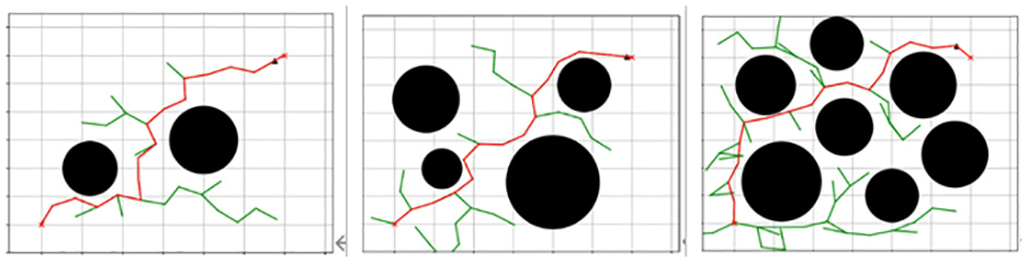
In Figure 10, we can see that Informed RRT* performs better under both loose and dense obstacles, achieving sub-optimal and optimal path length performance in terms of path length, respectively. But it also reaches the highest in time consumption. This is because the heuristic function of the Informed RRT* algorithm can effectively guide the search direction under both loose and dense obstacles, thus avoiding missing important paths and falling into local optimal solutions. In addition, using a mature tree structure for information transfer can improve the search efficiency and path quality. However, the computational complexity of the algorithms increases due to the need to compute the heuristic information, resulting in longer time-consuming.

Figure. 10.

Effectiveness diagram of Informed RRT* algorithm.

Overall, different algorithms perform significantly differently under different barrier densities. When choosing algorithms, it is necessary to balance path planning quality and computational complexity factors and flexibly select the appropriate algorithm according to the actual application scenarios.

Finally, using the line graph comparison method, the path lengths of the six algorithms mentioned above on the three types of obstacle maps, the algorithm time-consuming data were counted, the code was written in Python, and the line graphs were plotted using the matplotlib software.

According to Figure. 11, 12, path length or time can be used as the main evaluation indicators for the evaluation criteria, and another indicator can be used as an auxiliary indicator. Finally, Table 6 is produced.

Figure 11.

Line graph of path length for different obstacle maps.

Figure 12.

Time stacking diagram for different algorithms.

Table 6.

Characteristics of the six types of obstacle avoidance algorithms.

Property	Spare	Normal	Dense
A*	+	+++	+
Dijkstra	+	+	+
PRM	++	+	+++
RRT	-	-	-
RRT*	++	+++	++
Informed RRT*	+++	++	++

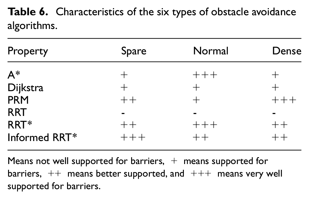
Means not well supported for barriers, + means supported for barriers, ++ means better supported, and +++ means very well supported for barriers.

Under loose barriers, PRM, Informed RRT*, and RRT* perform best, A* and Dijkstra perform worse, while RRT performs worst. RRT* has the shortest path length of these algorithms but takes the second longest time accordingly; Informed RRT* has the second longest path length, but its time performance is the longest. Therefore, when considering the balance between speed and path optimization, the Informed RRT* algorithm is chosen.

Under normal obstacles, all the algorithms perform close to each other, but PRM, RRT, and Informed_RRT* lag slightly behind. A*, Dijkstra, and RRT* demonstrate the best path length performance; however, their runtime is also longer. Hence, in this case, the A* algorithm is chosen.

All the algorithms perform poorly under dense barriers, but PRM, RRT*, and Informed RRT* exhibit better path length performance than others. The PRM algorithm was chosen considering the shorter running time of PRM. Furthermore, this means that path-planning algorithms need to work with sensors that can provide more map information for operation in complex spaces.

Choosing more suitable algorithms could be more efficient depending on the balance between the desired path length of time and the desired speed and path optimization. Such an analysis can inform applications, robotics, and autonomous vehicle decisions. Furthermore, based on the conclusion, selecting the most suitable algorithm for robot path-planning can provide a reference for robot sensor selection so that the selected sensor can compensate for the shortcomings of the algorithm and amplify its advantages.

In summary, this paper draws four conclusions:

• (1) If the path length is considered, the model will preferentially run the Informed RRT* algorithm on complex obstacle maps.

• (2) If the path length is considered, the model will preferentially run the RRT* algorithm on balanced obstacle maps.

• (3) If the algorithm time is considered, the model will preferentially run the A* algorithm on all obstacle maps.

• (4) If both aspects (path-planning, time-consuming) need to be considered, the model will run either the A* or PRM algorithm.

Conclusions

In this paper, a robot obstacle avoidance model based on a convolutional neural network is successfully studied using the joint deep learning convolutional neural network MobileNet_v3 and path-planning.

Eventually, it can be concluded from the experiment that if only the path length is considered, the model will prefer the Informed RRT* algorithm to deal with complex obstacle maps and the RRT algorithm to deal with normal obstacle maps. If only the algorithm time is considered, the model will prefer the A* algorithm to handle all the obstacle maps. If the combined consideration of path-planning and time consumption is needed, the model will choose the A* or PRM algorithm.

The results of the experiment provide a reference for the selection of path-planning algorithms, as well as some reference and inspiration for research in related fields, and also provide ideas for the selection of different algorithms in pathfinding. In subsequent research, further exploration can be conducted on integrating better deep learning models and path-planning algorithms and how to complement the shortcomings of different algorithms with different sensors to improve the obstacle avoidance ability and efficiency of robots in complex environments, making it applicable in more dynamic situations. ²⁵ This conclusion can also be applied to various fields, such as unmanned vehicles and smart homes.