Sage Journals: Discover world-class research

Abstract

Machining chatter is likely to occur during milling of thin-walled parts. The structural differences in thin-walled parts and the magnitude of the milling force can lead to varying degrees of chatter in different areas of the machining process. Predicting machining stability using dynamic modeling methods can be time-consuming. In this study, a method for establishing a particle swarm optimization-back propagation (PSO-BP) neural network model is proposed to predict the modal parameters of thin-walled parts and the surface vibration of machined parts. Based on measurements of the length, height, wall thickness, and position of the thin-walled parts, the modal parameters of the workpiece were predicted using the PSO-BP neural network model. Additionally, the average milling force was included as an input parameter to predict the displacement of surface vibrations on thin-walled parts using the PSO-BP model. The predictive results of the modal parameters and surface vibration displacement are evaluated using the evaluation function, which indicates that the PSO-BP neural network model can reliably predict the modal parameters and surface vibration depth of thin-walled parts.

Keywords

Thin-walled parts neural network modal parameters machining vibration

Introduction

Thin-walled parts are widely used in the aviation industry to reduce the weight and enhance the strength of parts.^1–3 To meet the demand for machining accuracy of the parts, thin-walled parts are usually machined by the milling method. Machining chatter occurs easily in the milling process because of the weak rigidity of the thin-walled structure. When chatter occurs, chatter remarks on the surface of the parts influence the machining quality of the parts, and the machining efficiency is reduced to decrease the machining chatter.^4,5 It is known that the machining quality and efficiency of thin-walled parts are limited by the machining chatter. Machining chatter prediction and suppression are the main problems to be addressed in the milling process of thin-walled parts.

The most widely used method for predicting the machining stability of parts is to establish a machining stability prediction model based on modal and machining parameters. Subsequently, the machining stability diagram can be achieved, and a reasonable spindle speed and axial cutting depth can be chosen to avoid machining chatter. The time domain method and the frequency domain method are the most widely used stability predicting method. Altintas and Budak^6,7 first proposed a machining stability prediction model for the milling process using a zero-order frequency-domain analytical method (ZOA). Based on the cutting parameters, the cutting force was predicted using the cutting force prediction model. The modal parameters of the machining tool can also be determined using impact tests. The stability of the milling process can be predicted, and the machining parameters can be optimized to avoid machining chatter using the stability lobe diagram. Insperger and Stépán^8,9 proposed a semi-discrete method to establish a stability prediction model for milling machining. Ding et al.¹⁰ developed a full-discretization method to predict the machining stability of milling in which the modal and cutting parameters were also determined. In this method, the stability lobe diagram can also be used to predict the machining chatter. Smith and Tlusty¹¹ established a time-domain simulation model for peak-to-peak cutting force values and used their variation as a criterion for chatter. Albertelli et al.⁵ carried out a chatter detection algorithm for nonstationary milling operations, and a cutting stability assessment was performed through the real-time computation of a normalized chatter indicator.

The machining stability prediction method mentioned above can be used to predict the machining chatter; however, in practice, machining chatter is more likely to occur during the machining of thin-walled parts. Therefore, in recent years, the prediction and suppression of machining chatter in thin-walled parts have become the focus of research on machining chatter. Dang et al.¹² proposed a method to analyze the machining stability of a pocked-shaped thin-walled part with a viscous fluid. The dynamic parameters of the cutter and parts were solved to establish the machining stability prediction model and avoid machining vibration by selecting reasonable parameters. Li et al.¹³ developed a flexible deformation prediction model for a thin-walled part and a multipoint contact dynamic model of a workpiece considering the deformation and location of the tool. Subsequently, a milling dynamic model is obtained to predict the machining chatter. Yuan et al.¹⁴ analyzed the forced vibration phenomenon and vibration shapes of thin-walled parts. Subsequently, the shear thickening fluid is applied to the thin-walled workpiece, and the vibration can be suppressed. Yang et al.¹⁵ predicted the in-process workpiece dynamics of thin-walled workpieces using the finite element method when the removed material was considered in the dynamic prediction of parts. Subsequently, the dynamic parameters were integrated to predict the machining stability during the milling process. Wan et al.¹ designed a moving fixture to enhance the stiffness and damping of a thin-walled workpiece that could move with the tool during the milling process. Then, a dynamic model of the workpiece considering the moving fixture is established, and the moving fixture can suppress the machining vibration of the thin-walled workpiece. According to the stability predicting theory, it can be known that the dynamics model can be established when the cutting force in milling process can be predicted and the modal parameters can be achieved by the impact tests.

With the development of artificial intelligence technology, an increasing number of artificial intelligence algorithms have been proposed and applied in the classification and prediction of research objects. Therefore, some intelligent algorithms have been applied to the prediction of chatter in thin-wall machining and the optimization of machining parameters. Hao et al.¹⁶ combined ensemble empirical mode decomposition and nonlinear dimensionless indicators to detect machining chatter in thin-walled parts. Cutting force signals were performed, and an improved support vector machine was developed to detect the chatter. Dun et al.¹⁷ developed an unsupervised method to detect machining chatter during the milling of thin-walled TC4 alloy workpieces. A hybrid clustering method based on both density and distance metrics was developed to cluster compressed signals. Machining chatter of thin-walled parts can be detected using this method. Sener et al.¹⁸ presented a chatter detection method for a deep convolutional neural network. The vibration data were collected and processed using a continuous wavelet transform (CWT). The deep convolutional neural network was trained and tested to predict machining chatter. Lu et al.¹⁹ developed an interpretable anti-noise convolutional neural network to detect chatter in a thin-walled workpiece milling process. An adaptive frequency-band attention module was designed based on the modal parameters and frequency spectrum. Subsequently, the discriminative feature attention module was used to recalibrate the feature responses of each convolutional layer, and milling experiments were conducted on the pocket-shaped thin-walled to verify the validity of the model. Zhang et al.²⁰ proposed a novel hybrid deep convolutional neural network that was combined with an inception module and a Squeeze-and-Excitation ResNet block. The inception module and Squeeze-and-Excitation ResNet block can extract features from the cutting force signals and assign weights to different feature channels separately. The accuracy of the model was improved using the two modules. The module can clarify the machining chatter using the cutting force signals and surface quality. Gupta and Singh²¹ developed a method to extract chatter features from turning sound signals. The processed signals can then be imported into the artificial neural network to predict the machining stability.

The modal parameters of the machining tool and thin-walled parts should be collected by impact tests in the dynamic machining stability prediction model and artificial intelligence algorithms. The most widely used modal parameter identification methods are mainly obtained through experimental approaches or finite element simulations. Butt et al.²² used an impact hammer to strike the tool position of a five-axis CNC machine. Then, the frequency response function and modal parameters can be acquired to assess the effect of eddy current damping on the modal parameters. Zhou et al.²³ conducted finite element simulation analysis of hollow and solid blades using Siemens NX software to obtain modal shapes and modal parameters. Based on this, a stability prediction model was established to forecast the milling stability of hollow blades. Although the geometry parameters of the thin-walled parts are significantly different, the modal parameters of thin-walled parts with different structures vary with the structure and position, as shown in Figure 1. Therefore, it is necessary to rebuild the geometric model and finite element model, or conduct modal testing methods to obtain the modal parameters. There is hardly any use of artificial intelligence algorithms to predict modal parameters. The period of stability prediction is long and the operation is complicated, which is not conducive to the practical application of the stability prediction method. Therefore, a machining stability prediction model that can determine whether machining vibrations occur is effective and significant when the structure and machining parameters in milling are confirmed.

Figure 1.

The frequency response curve of thin-walled parts with different size.

This study proposes a new method to predict the occurrence of chatter during the milling process of thin-walled parts based on their geometric dimensions and cutting forces. Unlike traditional dynamic modeling methods, this study employs a PSO-BP neural network model to predict chatter in the machining of thin-walled components. Using this model, the displacement caused by machining vibrations can be predicted by measuring the size of the thin-walled parts. First, the geometric dimensions of the thin-walled parts were obtained through measurement, including the length, height, wall thickness, machining location, and average cutting forces under different cutting parameters. Second, the modal parameters were acquired through hammer tests, and profile measurement tests were conducted to obtain the profile displacements of the workpiece surface caused by the machining chatter. Finally, a PSO-BP neural network model was developed to establish predictive models for both natural frequencies and machining surface profile displacements, and a reliability analysis of these models was conducted using evaluation functions.

Theoretical model

BP neural network model

Back propagation (BP) neural networks are most widely used in supervised learning, recognition, classification, and other fields.²⁴ The basic BP neural network mainly consists of an input layer, a hidden layer, and an output layer, as shown in Figure 2. The input and output parameters were determined, and the collected information was submitted to the input and output layers. The number and weights of the hidden layer nodes were determined using the evaluation function. The hidden layer can be trained using the input data, and the prediction accuracy can be improved.

Figure 2.

The diagram of BP neural network.

The input parameters are independent variables related to the structure of the parts and position of the machining tool. The input parameters are expressed as $x_{1}$ , $x_{2}$ , $x_{3}$ , $x_{4}$ , and $x_{5}$ . The output parameter and nodes of the hidden layer can also be expressed as $y$ and $θ_{1}$ , $θ_{2}$ , $θ_{3}$ . The connection weight coefficient of the hidden layer can be compared and optimized when the input data are imported and the neural network is trained. The number of neurons in the q layer is n, and the connection weight coefficient for the ith neuron input to the $q$ layer is $w_{ij}^{q}$ . The transformation relationship between the input and output parameters can be expressed as

y_{i}^{q} = \sum_{j = 0}^{n - 1} w_{ij}^{q} x_{j}^{q - 1}

(1)

Suppose the input and output samples of the p group are given to train the BP neural network; the samples are $x = [x_{p 1}, x_{p 2}, x_{p 3}, \cdot \cdot \cdot x_{pm}]$ and $y = [y_{1}, y_{2}, y_{3}, \cdot \cdot \cdot y_{p}]$ . The samples can then be used to train the neural network, and the connection weight coefficient can be learned and refreshed. The relationship between the input and output parameters is established. The cost function of the fitting error function is.

E_{p} = \sum_{i = 1}^{n} (y_{pi} - y_{i})^{2}

(2)

Where $E_{p}$ is the fitting error between the predicted results and the output samples, $y_{pi}$ is the calculated results of the fitting model, $y_{i}$ is the output samples.

Particle swarm optimization (PSO)

PSO is introduced to the neural network to optimize the connection weight coefficient of the hidden layer. According to the connection weight of each particle, the prediction error of the neural network was calculated as the fitness function. Then, the position and velocity of the particle are updated according to the current position and velocity of the particle, as well as the global and individual optimal positions. The new connection weight is calculated according to the updated particle position, and the optimized connection weight is obtained.

An appropriate fitness function is selected, and the fitness value for each particle in the population is solved. If the new fitness value is less than the current fitness value, the current position is replaced with the new position. Subsequently, the particle position with the best fitness value in the population was selected as the global best position. The position $P^{i}$ and velocity of each particle $v^{i}$ were iterated according to the following formula:

v^{i} = u v^{i} + c_{1} r_{1} (p_{ibest} - x^{i}) + c_{2} r_{2} (G_{best} - x^{i})

(3)

P^{i} = P^{i} + v^{i}

(4)

Where $u$ is the Inertia factor, $c_{1}$ and $c_{2}$ are the acceleration factors, $r_{1}$ and $r_{2}$ is two random numbers varying within [0, 1]. $p_{ibest}$ is the historical best position experienced by the ith particle, and $G_{best}$ is the best location in history that the group has ever experienced.

PSO-BP neural network model

The basic idea of the PSO-BP neural network is to use the PSO algorithm to optimize the weights and thresholds of the BP neural network. The number of neurons in the input, hidden, and output layers can be set, and the weights and thresholds of the network can be initialized. Then, the number of particles is defined, and the position (weights and thresholds) and velocity of each particle are initialized. The BP algorithm is used to calculate the fitness value (e.g. mean square error) for each particle position. If the fitness of the current particle is better than its personal best, the personal best is updated. If the fitness of any particle is better than the global best, the global best position is updated. If the stopping criteria are satisfied (e.g. maximum iterations reached or satisfactory fitness), proceed to the next step. Otherwise, return to iteration. Therefore, the weights and thresholds corresponding to the global best position as the optimized parameters are returned to the BP neural network. A diagram of the PSO-BP neural network is shown in Figure 3.

Figure 3.

The diagram of PSO-BP neural network algorithm process.

When training a BP network using the PSO algorithm, the elements of the position vector X of the particle swarm are the overall connection weights and thresholds of the BP network. First, the position vector X is initialized, and the PSO algorithm is used to search for the optimal position such that the mean square error indicator shown in equation (5) reaches a minimum and the fitness value is minimized.

T = \frac{1}{N} \sum_{i = 1}^{N} \sum_{j = 1}^{C} (s_{ij}^{q} - s_{ij})^{2}

(5)

Where $N$ is the number of samples in the training set, $s_{ij}^{q}$ is the ideal output value of the $j$ th network output node of the $i$ th sample, $s_{ij}$ is the actual output value of the $j$ th network output node of the $i$ th sample, and $C$ is the number of neuron outputs by the network.

Proposed chatter predicting method

Flow of milling chatter prediction

The proposed chatter detection method is illustrated in Figure 4. The flow of milling chatter prediction comprises data processing, model construction, and chatter prediction. The length, width, and height of the thin-walled parts and the position of the parts were set as the input data of the model. Because of the influence of the connection area and structure on the workpiece, the response function at different positions of the workpiece will be significantly different; therefore, when the input parameters are different, the modal parameters will be different. Two prediction models for the machining chatter were established. One model takes the dimensions of thin-walled parts as input and outputs modal parameters, whereas the other model uses the dimensions of thin-walled parts and cutting forces as inputs to output machining vibration displacement. The modal parameters were then set as output parameters in the prediction model. Simultaneously, the surface mark on the surface is determined by the different response displacements of the tool to the workpiece. According to the analysis of the dynamic equation of the milling process, the machining stability is related to the excitation force in the machining process, as shown in equation (6).

m \overset{\cdot\cdot}{x} + c \overset{\cdot}{x} + k = F

(6)

where $m$ , $c$ , and $k$ are the mass, damping, and stiffness, respectively; $F$ represents the cutting force in the machining process; and $\overset{\cdot\cdot}{x}$ , $\overset{\cdot}{x}$ is the acceleration and velocity. Therefore, the cutting force should also be considered as an input parameter when the machining displacement of the surface mark is set as the output parameter. The prediction model can be constructed as described in Section “Theoretical model” when the input and output parameters are collected, and the fitting errors can be optimized to make the training data agree with the predicted results.

Figure 4.

Flow of proposed chatter predicting method.

Experiment set-up

In the modal measuring experiments, a Benstone VP5 dynamic signal analyzer was used to collect the response signal of the thin-walled parts. The accelerator of IMV VP-A1PO was used to stick to the workpiece surface to measure the acceleration, and the PCB 086c03 impact hammer exerted an exciting force on the workpiece by hammering the target area. Modal measuring experiments of plate thin-walled parts were implemented using a dynamic signal analyzer, acceleration sensors, and impact hammer, as shown in Figure 5(a).

Figure 5.

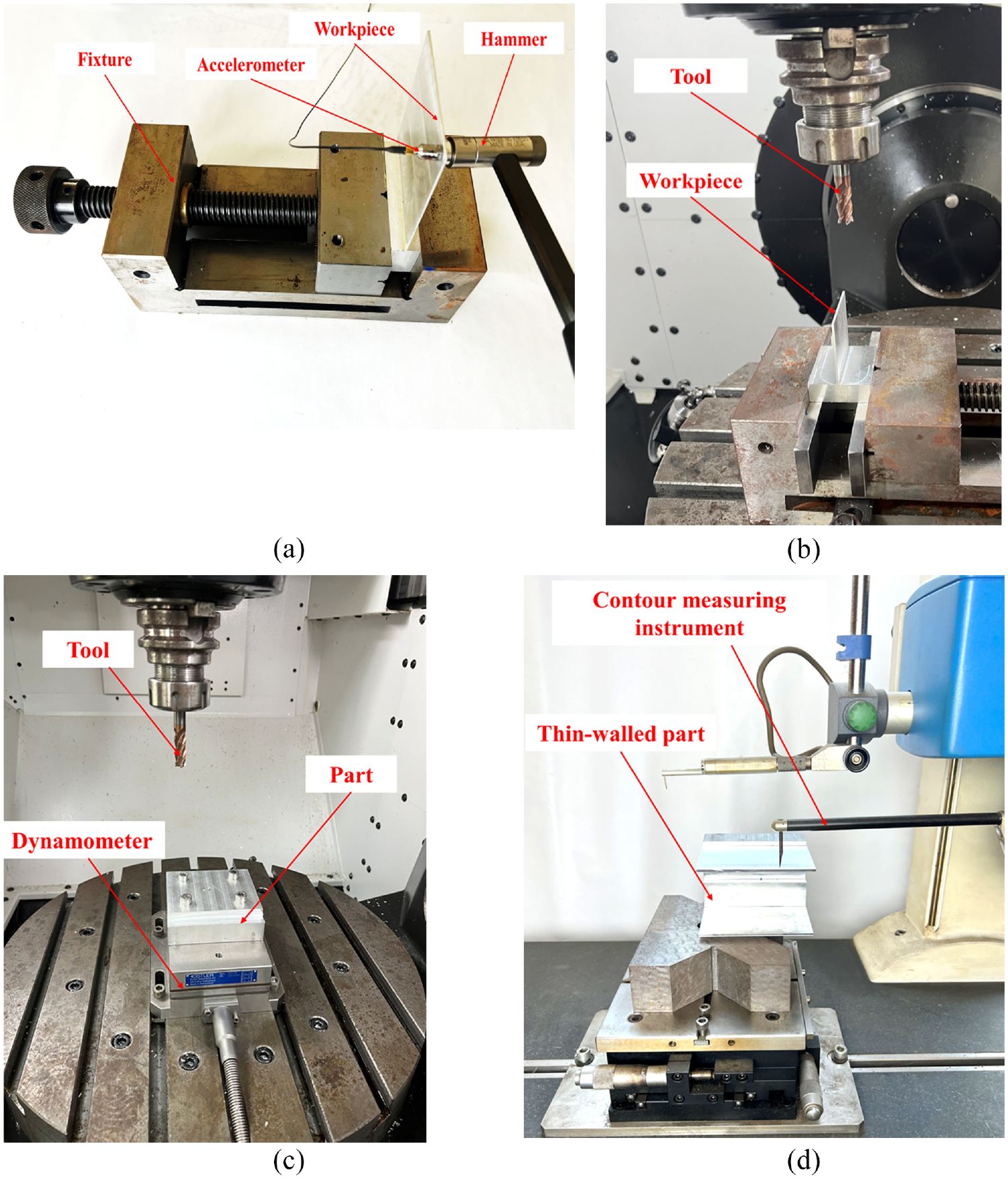
Experiment setup of modal measuring and milling experiment: (a) modal measuring experiments, (b) thin-walled part machining experiment, (c) the milling force measuring experiment, and (d) the contour measuring experiment.

Thin-walled aluminum alloy parts of different sizes were used to measure the modal response of the system and machining vibrations. After the modal measurement experiments, the parts were machined using a Mikron MILL E 500 U five-axis milling machine. The selected milling tool is a 4-tooth end mill with a diameter of 10 mm and the sizes of the selected thin-walled parts are 80 mm × 50 mm × 1.5 mm, 275 mm × 70 mm × 2.5mm, 50 mm × 50 mm × 1.5 mm, 100 mm × 70 mm × 2 mm, 100 mm × 70 mm × 2.5 mm, 100 mm × 60 mm × 3 mm, 200 mm × 50 mm × 1.5 mm, 200 mm × 70 mm × 2.5 mm. According to the size of the thin-walled part, the workpiece is evenly divided based on its length and height, with five measuring points in the length direction and three measuring points in the height direction. A machining diagram of the thin-walled parts is shown in Figure 5(b). To remove the influence of deformation and chatter of thin-walled parts during milling and obtain the cutting force of the aluminum alloy in a stable state, the non-thin-walled aluminum alloy parts were cut by changing the cutting parameters, and the milling force was obtained using a Kistler 9257 B dynamometer, as shown in Figure 5(c). The thickness of the thin-walled parts after machining can be measured, and the profile of the thin-walled parts can be obtained using Hommel T8000 roughness and profile measuring instruments, as shown in Figure 5(d).

The modal response of thin-walled workpieces

Impact experiments of thin-walled parts with different structures were designed to acquire the modal response of the thin-walled parts. The accelerator can be fixed to the surface of the parts when the length, width, and height of the parts are measured. Because the modal responses of different positions are different, the accelerators are evenly distributed at a certain distance along the height and length directions to obtain modal responses at different locations. Therefore, the sensors were arranged in several layers. The layout design of the sensor on the thin-walled parts of the different structures is shown in Figure 6. According to the length and height dimensions of the thin-walled parts, three measurement positions were evenly distributed along the height direction on the machined surface of the thin-walled parts, and five measurement positions were evenly distributed along the length direction. In total, 15 measurement points were obtained for each thin-walled part. Owing to the lack of boundary support at the edges of the workpiece, deformation and vibration can easily occur during machining; therefore, the measuring points near the edge are located 10 mm away from the edge.

Figure 6.

Modal measuring experiments of thin-walled plate part.

The real and imaginary parts of the frequency response function can be seen in Figure 7 when the length, height, and width of the plate part are 200, 50, and 1.5 mm. It can be known from Figure 7(a) that the frequencies of the first peak and trough are 525 and 533.8 Hz, respectively. Then, the maximum peak value and the minimum trough value of the real part corresponding to the first-order natural frequency are 195.9 and −52.36 mm/s². The imaginary parts of the frequency response function can be known from Figure 7(b). The minimum value of the first-order frequency is −174.8 mm/s² and the frequency is 527.5 Hz. It can be observed from Figure 7(a) and (b) that the first-order natural frequency is 527.5 Hz. According to the calculation formula for the natural frequency, the natural frequency is related to the stiffness and quality of the machined object and can reflect the modal performance of the thin-walled part.

Figure 7.

Modal response curve of the plate part (length is 200 mm, height is 50 mm, and width is 1.5 mm): (a) real part of frequency response function and (b) imaginary part of frequency response function.

The frequency response function curves measured at points A and B on the workpiece are shown in Figure 8. Point A is located at approximately 10 mm in length and 40 mm in height, while point B is located at approximately 100 mm in length and 25 mm in height. The measured curve at point A shows a natural frequency similar to that at point B; however, its peak value is significantly higher than that at point B. The response peak at point A is approximately 132.9 mm/s²/N, while the corresponding peak at point B is about 33.23 mm/s²/N. Since point A is close to the edge of the workpiece, it has lower rigidity and a higher response peak, whereas point B is near the center of the workpiece, resulting in a lower response peak.

Figure 8.

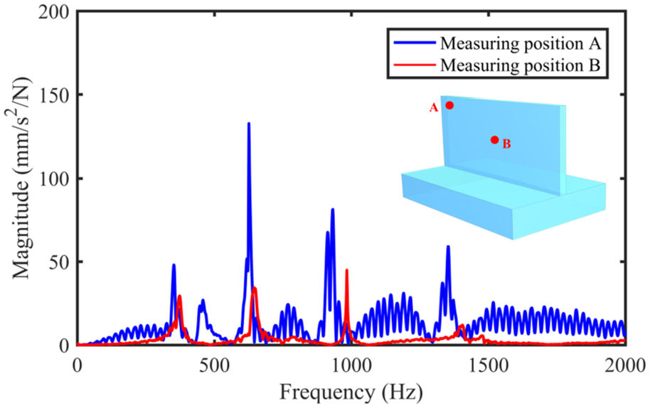
Comparison of workpiece frequency response curves at different measurement positions.

The chatter response of system

To establish the PSO-BP model between the workpiece geometry and machining vibration displacement response, thin-walled parts with various specifications were milled. Subsequently, through measurement, the cutting force data and surface profile data of thin-walled parts under different machining parameters were collected. The measured results of the cutting force and surface profile when the length, height, and width of the plate part are 200, 50, and 1.5 mm, respectively, are shown in Figure 9.

Figure 9.

The measured cutting force and surface profile results: (a) the cutting force result and (b) the surface profile result.

When the axial cutting depth was 5 mm, radial cutting depth was 1 mm, spindle speed was 3000 rpm, and feed rate was 200 mm/min, the cutting force data were collected. The normal component force was analyzed owing to its significant influence on the dynamic deformation of the workpiece surface when the thin-walled part was machined. The cutting force along the direction normal to the workpiece surface is shown in Figure 9(a). From the analysis of the figure, it can be seen that the maximum cutting force in one rotation of the tool is 3.26 N, and the minimum cutting force is −23.7 N. To facilitate the construction of the subsequent model, the average cutting force was set −20.4 N. The cutting force data were used as input data in the subsequent model construction, and the milling force of the aluminum alloy is listed in Table 1. To study the vibration of the workpiece after machining, the height of the surface vibration mark after machining, thickness of the workpiece after machining, and surface profile were measured. The measurement results for the workpiece surface profile are shown in Figure 9(b). In the measurement range of 3 mm, the peak of one surface profile was 0.036 mm, and its corresponding valley was −0.009 mm. The difference between the surface profiles of the two points was 0.045 mm. The results show that thin-walled parts exhibit machining vibrations during machining. For parts with relatively high machining accuracy, this exceeds the surface accuracy requirements of the workpiece. The measured distance between the two points was 0.39 mm. The machined surface of the thin-walled part is illustrated in Figure 10.

Table 1.

The average cutting force of the aluminum alloy.

Variables	$a_{p}$ (mm)	$a_{e}$ (mm)	$n$ (r/min)	$f$ (mm/min)	Cutting force (N)
1	3	0.5	5000	300	23.5
2	2	0.5	3000	100	14
3	1.5	1	2500	250	20.1
4	1	1.5	3000	300	20
5	0.5	1.5	4000	400	10.3
6	5	1	3000	200	20.4

Figure 10.

The machined surface of thin-walled part.

Training and performance

Model parameters

To train and test the model more accurately, 120 data sets were selected to train and test the natural frequency. Among them, 84 groups were randomly selected for model training, and the remaining 36 groups were used as the test sets. In these sets of data, the length, width, and height of the workpiece and the position of the modal measurement were set as the input parameters, and the natural frequency of the impact experiment was set as the output parameter. In the BP algorithm, the maximum number of training sessions was set to 500, the target error was set to $1 \times 10^{- 6}$ and the learning rate was set to 0.01. The number of nodes in the hidden layer was selected as five according to the number of parameters in the hidden layer is selected as five. In the process of parameter optimization using the PSO algorithm, the learning factor of the model was set to 4.5, the number of population updates was set to 45, the size of the population was set to five, and the optimization speed ranged from −1 to 1.

Verification of the method

Modal verification

After the above parameters were used for training and verification, a comparison diagram between the model prediction results and actual measurement results was obtained, as shown in Figure 11(a) and (b). When the geometric parameters (length of 200 mm, height of 50 mm, and width of 1.5 mm) are determined, a comparison of the training results for natural frequencies can be seen in Figure 11(a), and a comparison of the testing results for natural frequencies is shown in Figure 11(b).

Figure 11.

The evaluation of the training and testing model for modal parameters: (a) comparison of the training results for natural frequencies, (b) comparison of the testing results for natural frequencies, (c) accuracy of the train model, and (d) accuracy of the test model.

The coefficient of determination (R²), root mean square error (RMSE), mean absolute error (MAE), and mean absolute percentage error (MAPE) were used to evaluate the accuracy of the model predictions. The coefficient of determination (R²) is typically used to evaluate the efficiency of a neural network model.²⁴ When the value is close to 1, it can be known that the predicting result is in agreement with the actual result. The Root Mean Square Error (RMSE), Mean Absolute Error (MAE), and Mean Absolute Percentage Error (MAPE) are three evaluation functions often used to evaluate the performance of regression models. RMSE measures the square root of the average squared differences between the predicted and actual values, giving higher weights to larger errors and indicating the overall model accuracy. The MAE calculates the average absolute differences between the predicted and actual values, providing a straightforward interpretation of the average error without emphasizing larger discrepancies. The MAPE expresses the error as a percentage, which helps in understanding the relative accuracy of the model, making it easily interpretable across different scales. Together, these metrics offer a comprehensive view of model performance, highlighting different aspects of prediction accuracy. The RMSE, MAE, and MAPE are the equations for the four metrics as follows:

\begin{matrix} R^{2} = 1 - \frac{\sum_{i = 1}^{n} {(x_{i}^{'} - x_{i})}^{2}}{\sum_{i = 1}^{n} {({\bar{x}}_{i} - x_{i})}^{2}} \end{matrix}

(7)

RMSE = \sqrt{\frac{1}{n} \sum_{i = 1}^{n} {(x_{i}^{'} - x_{i})}^{2}}

(8)

MAE = \frac{1}{n} \sum_{i = 1}^{n} | x_{i} - x_{i}^{'} |

(9)

MAPE = \frac{1}{n} \sum_{i = 1}^{n} \frac{| x_{i}^{'} - x_{i} |}{x_{i}}

(10)

Where $n$ is the number of data points in the sample, ${\bar{x}}_{i}$ is the mean value of the actual measurement results, $x_{i}^{'}$ is the predicted value of the model, and $x_{i}$ is the value of the actual measurement results.

A total of 120 data sets were used as samples to train and test the model for natural frequencies. From these 120 data sets, 84 sets of data were selected as the training group, while 36 sets of data were designated as the testing group. The R² values of the training and testing model are 0.98 and 0.92. This shows that the training and testing models matched the actual values very well. Therefore, the model was highly reliable. The MAE of the training and testing model were 12.39 and 30.55, respectively. The RMSE of the training and testing model are 21.21 and 46.59. The MAPE values of the training and testing models are 0.099 and 0.171, respectively. The value of this natural frequency is larger, and thus, the MAE and RMSE values are more obvious. After converting the basic values into percentages, it was found that the accuracies of the training and test models were higher.

Chatter displacement verification

To establish the relationship between parameters such as workpiece geometrical size, tool position, cutting force, and workpiece surface vibration, a PSO-BP neural network model was established. In this model, the geometrical size of the workpiece, tool position, and cutting force were set as the input parameters. The height of the surface chatter mark is set as the output parameter. In the 120 sets of data, 84 groups were selected as the training group and 36 groups were set as the testing groups. The initial parameters and evaluation indices of the model were consistent with those of the modal parameter prediction model. A neural network model was established and the results are shown in Figure 12.

Figure 12.

The evaluation of the training and testing model for modal parameters vibration marks on the surface of the workpiece: (a) comparison of training results for vibration marks, (b) comparison of testing results for vibration marks, (c) accuracy of the train model, and (d) accuracy of the test model.

It can be seen from Figure 12(a) and (b) that the predicted surface profiles of the milled thin-walled parts are basically the same as the measured data. The input and output data in Figure 12(a) are 84 groups of data, and the input and output data in Figure 12(b) are 36 groups of data. The maximum displacement of the parts induced by the machining chatter was 0.06 mm. Based on the machining accuracy of thin-walled parts, the surface quality of the workpiece machining accuracy caused by machining vibration is poor. The machining accuracy of thin-walled parts cannot satisfy the requirements of the workpiece. Simultaneously, the calculation results for the error function of the model were obtained. The R² values of the training and testing model are 0.62 and 0.608, respectively. The MAE values of the training and testing models are 0.005 and 0.005, respectively. The RMSE of the training and testing models are 0.007 and 0.008, respectively. The MAPE values of the training and testing model were 0.38 and 0.42.

The solution accuracy of the model is lower than that of the natural frequency prediction model, which may be due to the fact that the measurement results of the output values in the model are the average of multiple surface profile measurements. The measured results are then scattered, which increases the difficulty of fitting and results in a large error in the prediction results, as shown in Figure 12(c) and (d).

Comparison with other method

To study the accuracy of the prediction results of the PSO-BP neural network model, a BP neural network model was established with natural frequency as output data and the length, height, and wall thickness of the thin-walled parts as input parameters. The predicted results were compared with those of the PSO-BP neural network model, as shown in Figure 13. The R² values of the PSO-BP and BP training model is 0.98 and 0.87. The MAE of the training models was 12.39 and 0.43. The RMSE of the training and testing model are 21.21 and 61.26. The MAPE values of the training and testing models are 0.099 and 0.198, respectively. The R² value of the PSO-BP model was closer to 1, and the errors of the predicted results for the PSO-BP neural network model were smaller than those of the BP neural network model. The evaluation functions show that the predicted results of the PSO-BP model have higher accuracy than the predicted results of the BP model.

Figure 13.

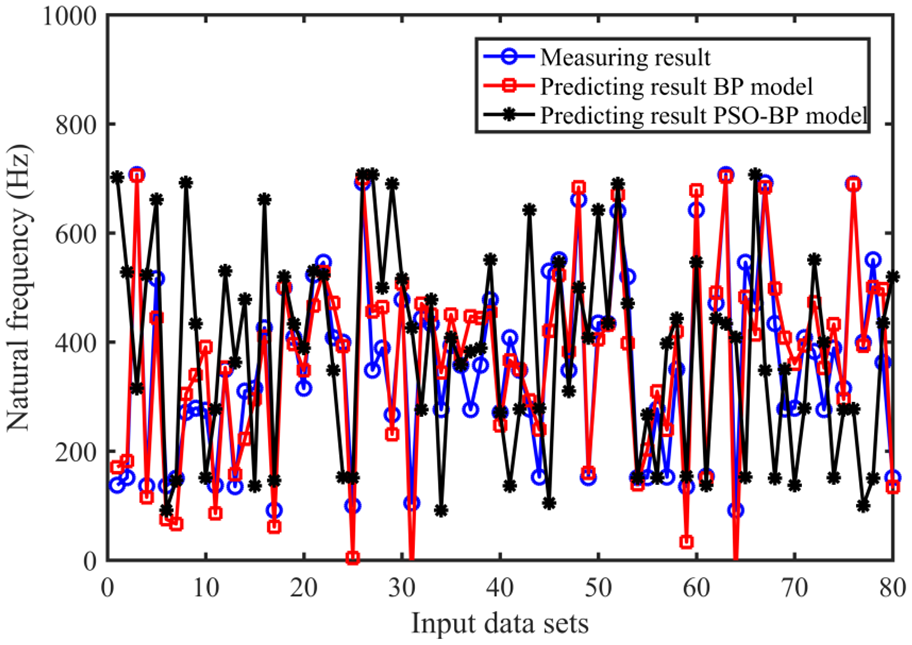
Comparison of PSO-BP and BP neural network model.

Conclusion

The artificial neural network model is an artificial intelligence model that achieves output prediction by determining the hidden-layer coefficients based on the input and output data. The machining process of thin-walled parts is prone to chatter, and it is difficult to predict whether chatter will occur during machining before parts are machined. Therefore, ensuring the quality of thin-walled parts is a challenge. Using an artificial intelligence neural network model to predict machining chatter can effectively forecast whether chatter will occur before thin-walled parts are machined, making it an effective method for predicting machining chatter. The main conclusions drawn from this study are as follows:

(1) Through experiments measuring the dimensions of thin-walled parts, modal measurements, and surface profile measurements of the machined workpieces, data on the length, height, position, natural frequency, and surface vibration displacement of the thin-walled workpieces were obtained, thereby providing the necessary data for the establishment of the PSO-BP neural network model.

(2) A PSO-BP neural network model was established with the length, height, and position of the thin-walled workpiece as input parameters and the natural frequency as the output parameter. This model can be used to predict the natural frequency of plate-like thin-walled parts. Analysis of the model’s evaluation function revealed an R² value of 0.98 and an MAPE of 0.099 for the training set, while the traditional BP model yielded an R² value of 0.87 and an MAPE of 0.198 for the training set. The prediction accuracy of the PSO-BP model was significantly higher than that of the traditional BP neural network model.

(3) A PSO-BP neural network model was established with the length, height, position, and cutting force of the thin-walled workpiece as input parameters and the surface profile error as the output parameter. This model can predict the surface errors caused by machining vibrations. The analysis showed an R² value of 0.62 and a MAPE of 0.38 for the training set.

Footnotes

Handling Editor: Jinting Xu

Author contributions

Junming Hou: Writing – original draft preparation and methodology. Baosheng Wang: Conceptualization, Data curation, formal analysis. Dongsheng Lv and Changhong Xu: Writing – review and editing.

Declaration of conflicting interests

The author(s) declared no potential conflicts of interest with respect to the research, authorship, and/or publication of this article.

Funding

The author(s) disclosed receipt of the following financial support for the research, authorship, and/or publication of this article: This work was partially supported by the Key University Science Research Project of Jiangsu Province, China (21KJA460011, 22KJA460006) and the Research Fund of the Nanjing Institute of Technology (ZKJ202103).

Data availability statement

The datasets generated during the current study are available from the corresponding author upon reasonable request.

ORCID iD

Junming Hou

References

Wan

Dang

Zhang

, et al. Chatter suppression in the milling process of the weakly-rigid workpiece through a moving fixture. J Mater Process Technol 2022; 299: 117293.

Yan

Hao

Zhu

, et al. Towards high milling accuracy of turbine blades: a review. Mech Syst Signal Process 2022; 170: 108727.

Hou

Zhao

, et al. Machining stability enhancement in multi-axis milling of titanium hollow blade by introducing multiple damping and rigid supporters. J Manuf Process 2021; 64: 198–208.

Wang

Wan

Zhang

, et al. Chatter detection methods in the machining processes: a review. J Manuf Process 2022; 77: 240–259.

Albertelli

Braghieri

Torta

, et al. Development of a generalized chatter detection methodology for variable speed machining. Mech Syst Signal Process 2019; 123: 26–42.

Altintaş

Budak

Analytical prediction of stability lobes in milling. CIRP Ann Manuf Technol 1995; 44: 357–362.

Altintas

Budak

Analytical prediction of chatter stability in milling-part I: general formulation. J Dyn Syst Meas Control 1998; 120: 22–30.

Insperger

Stépán

Semi-discretization method for delayed systems. Int J Numer Methods Eng 2010; 55: 503–518.

Insperger

Stépán

Updated semi-discretization method for periodic delay-differential equations with discrete delay. Int J Numer Methods Eng 2004; 61: 117–141.

10.

Ding

Zhu

Zhang

, et al. A full-discretization method for prediction of milling stability. Int J Mach Tools Manuf 2010; 50: 502–509.

11.

Smith

Tlusty

Efficient simulation programs for chatter in milling. CIRP Ann Manuf Technol 1993; 42: 463–466.

12.

Dang

Wan

Zhang

, et al. Chatter analysis and mitigation of milling of the pocket-shaped thin-walled workpieces with viscous fluid. Int J Mech Sci 2021; 194: 106214.

13.

Wang

Chatter prediction in flank milling of thin-walled parts considering force-induced deformation. Mech Syst Signal Process 2022; 165: 108314.

14.

Yuan

Wang

Mao

, et al. Forced vibration mechanism and suppression method for thin-walled workpiece milling. Int J Mech Sci 2022; 230: 107553.

15.

Yang

Zhang

, et al. An efficient decomposition-condensation method for chatter prediction in milling large-scale thin-walled structures. Mech Syst Signal Process 2019; 121: 58–76.

16.

Hao

Zhu

Yan

, et al. Milling chatter detection with WPD and power entropy for Ti-6Al-4V thin-walled parts based on multi-source signals fusion. Mech Syst Signal Process 2022; 177: 109225.

17.

Dun

Zhu

Yan

, et al. A chatter detection method in milling of thin-walled TC4 alloy workpiece based on auto-encoding and hybrid clustering. Mech Syst Signal Process 2021; 158: 107755.

18.

Sener

Gudelek

Ozbayoglu

, et al. A novel chatter detection method for milling using deep convolution neural networks. Measurement 2021; 182: 109689.

19.

Xiong

LZ.

An interpretable anti-noise convolutional neural network for online chatter detection in thin-walled parts milling. Mech Syst Signal Process 2024; 206: 110885.

20.

Zhang

Gao

Hong

, et al. Improving generalisation and accuracy of on-line milling chatter detection via a novel hybrid deep convolutional neural network. Mech Syst Signal Process 2023; 193: 110241.

21.

Gupta

Singh

Investigation of tool chatter using local mean decomposition and artificial neural network during turning of Al 6061. Soft Comput 2021; 25: 11151–11174.

22.

Butt

Yang

Pei

, et al. Five-axis milling vibration attenuation of freeform thin-walled part by eddy current damping. Precis Eng 2018; 51: 682–690.

23.

Zhou

Zhang

Luo

, et al. Toolpath dependent chatter suppression in multi-axis milling of hollow fan blades with ball-end cutter. Int J Adv Manuf Technol 2014; 72: 643–651.

24.

Mulumba

Liu

Hao

, et al. Application of an optimized PSO-BP neural network to the assessment and prediction of underground coal mine safety risk factors. Appl Sci 2023; 13: 5317.

Prediction of vibration in milling of thin-walled aluminum alloy parts using neural network model

Abstract

Keywords

Introduction

Theoretical model

BP neural network model

Particle swarm optimization (PSO)

PSO-BP neural network model

Proposed chatter predicting method

Flow of milling chatter prediction

Experiment set-up

The modal response of thin-walled workpieces

The chatter response of system

Training and performance

Model parameters

Verification of the method

Modal verification

Chatter displacement verification

Comparison with other method

Conclusion

Footnotes

Author contributions

Declaration of conflicting interests

Funding

Data availability statement

ORCID iD

References