Sage Journals: Discover world-class research

Abstract

The fatigue evaluation of the bogie frame is an important part of the structural health monitoring of the vehicle. During the dynamic stress monitoring, some signal spikes, which are much larger than the normal fluctuation range due to the interference of the complex electromagnetic environment, affect the accuracy of the structural damage assessment and need to be accurately detected and replaced. Aiming at the drawbacks of traditional detection methods that are overly dependent on engineering experience and not universal, a novel spike detection model is proposed in this paper. By the process of data transformation, spike region features are effectively separated. Based on the isolation forest algorithm, the normalized anomaly score of each point is calculated, and the threshold is determined adaptively. The spike detection rate and damage sensitivity are proposed as the evaluation indices of the detection effect of the method. The results show that the spike detection rate is improved by 7.86% on average, and the damage sensitivity is improved by 15.59% on average. The spike detection model in this paper is significantly improved compared to the existing methods.

Keywords

Bogie frame dynamic stress signal monitoring signal spike detection instantaneous rolling weighted standard deviation isolation forest

Introduction

As a key structure of the rail vehicle running part, the bogie frame is subjected to a variety of loads such as floating, rolling, braking, traction, and other coupling effects in the process of application, while the frame is an all-welded structure, and the fatigue strength of the weld region is much smaller than that of the base material due to the influence of the residual stresses, stress concentrations, and weld defects, which results in frequent cracks in the frame before it reaches the design life,^1,2 and brings a great challenge to the vehicle operation safety.

In terms of structural health monitoring of the bogie frame, to accurately evaluate the damage level of the frame under the current operating conditions, the real dynamic stress of the frame can be obtained by sticking strain gauges in the key regions. The monitoring quality of the real dynamic stress signal determines the accuracy of the final structural damage evaluation, in which the factors affecting the signal monitoring quality mainly focus on two aspects. On the one hand, at the beginning of the actual monitoring process, the strain gauges need to be preheated, and the external ambient temperature may change greatly during the monitoring process, resulting in a significant zero drift of the real dynamic stress signal.³ On the other hand, the connecting cables of the dynamic stress monitoring system are in a complex electromagnetic compatibility environment, for example: a large number of electromagnetic radiation interferences are generated by lifting and lowering pantographs and over-phase operations, and conductive interferences are also generated by electrical equipment under the vehicle through cables,^4–6 which result in a large number of randomly located outliers, that is, spikes, in the dynamic stress signals. When the real dynamic stress signal is mixed with the above two interfering components, especially the signal spikes, the accuracy of the structural damage assessment will be greatly affected. Specifically, since the spike signal in the time domain shows high frequency and large amplitude oscillations in a short time, if the measured stress spectrum is constructed for the dynamic stress data containing signal spikes, the frequency of the stress spectrum block with large range cycles will be significantly increased, which will lead to the damage value being too large and the fatigue evaluation results being distorted. Due to the duration, fluctuation range, frequency distribution, and other characteristics of the signal spike in the dynamic stress data are not consistent, the detection of dynamic stress signal spike has a high degree of complexity. At present, in the actual engineering application, the spike detection method for the measured dynamic stress signal has not yet been formed, and it generally relies on the engineering experience of the researchers to mark and process manually, and the quality and efficiency of the data processing need to be improved urgently.

Signal spikes are typical time series anomalies, which are usually characterized by the following features as defined in the literature.^7–9 The different types of anomalies can be divided into point anomalies, collective anomalies, and contextual anomalies, of which signal spikes correspond to the first two types of anomalies according to different causes. The signal spike detection problem generally consists of a forward problem and an inverse problem. The forward problem is to locate the signal spike location based on the original data in the time domain, and a typical application is the electroencephalogram (EEG) signal spike determination.¹⁰ The inverse problem, that is, estimating and reconstructing the physical information and characteristics in the original data based on the inclusion of noisy signals or images represented by signal spikes, involves the process of sparse deconvolution.¹¹ Good results have been achieved with Gaussian mixture models,¹² non-negative Bayesian learning,¹³ and non-convex sparse regularization.¹⁴

For the forward problem, in recent years, researchers have carried out extensive studies on the problem of anomaly detection, and this paper classifies the basic algorithm models, as shown in Table 1.

Table 1.

Classification of anomaly detection models.

No	Model class	Algorithm class	Basic algorithm name	Citations
I	Statistics	Distribution-based	Z-score/HMM/SKL divergence	^15–19
II	Classical machine learning	Prediction-based	ARMA/ARIMA/PCI/Bayesian-DLM	^20–23
		Classification-based	SVDD/NSVDD	^24,25
		Distance-based	KNN	^26,27
		Density-based	LOF	²⁸
		Cluster-based	K-means	^29,30
		Dimensionality reduction-based	PCA	³¹
		Tree-based	Random forest/isolation forest	^32–36
III	Neural network (deep learning)	Supervised	LSTM/Bayesian-CNN/ANN	^37–39
III	Neural network (deep learning)	Unsupervised	Auto-encoder	^40,41

Although a series of time series outlier detection models with good results have been developed in various fields, especially in the field of SHM, there are still the following challenges in applying them to the problem of frame dynamic stress signal spike detection.

(1) In the existing literature, the experimental data used in the outlier detection models are mainly derived from test stand tests (e.g.^15,24,29) or publicly available data sets (e.g.^25,26,37), which do not require complex pre-processing of the data for the application of these detection models. However, the frame dynamic stress signals are affected by the field environment and contain specific internal interference components, such as 50 Hz power-line interference, zero drift, and signal oscillation due to vehicle start-stop transients may cause local peaks in the signal due to the superposition of these interfering components, which may lead to a large number of misjudgments in the model during the spike detection process. Since there are many types of interference components and the causes of interference components are closely coupled with the field test conditions, the various types of interference components in the pre-processing stage have not yet been strictly classified, and the time-frequency characteristic law of each type of interference component lacks a specific mathematical description, so it is difficult to solidify the processing flow corresponding to each type of interference component. In addition, for each type of interference component, there is no appropriate index to quantitatively judge the quality of the pre-processing results, and it is difficult to control the accuracy of the forward link of signal spike detection.

(2) The duration of the dynamic stress monitoring process of the bogie frame is long, the signal sampling rate is above 1000 Hz, and the number of single-channel data points is usually above ten million, which is much larger than the scale of the test data in the literature, whereas the algorithm complexity of the detection algorithms in the literature is generally high, and the computational time overhead is too large when facing the task of detecting long-time sequence outliers.

(3) In order to quantitatively evaluate the detection effect of model outliers, different literatures have constructed a variety of evaluation indices according to the characteristics of the data to be detected, for example, MCC, F0,³⁷ elastic loss, vulnerability and duration.¹⁶ The calculation method of these evaluation indices is closely related to the type of data to be detected, the way of anomaly statistics, etc., and cannot be directly applied when evaluating the effectiveness of dynamic stress signal spike detection.

To solve the above problems, this paper proposes a detection model for signal spikes oriented to the dynamic stresses of bogie frames, and its main contributions can be summarized as follows:

(1) The trend removal method (TRM) is constructed for the zero-point drift phenomenon in the original signals of dynamic stress based on the segmented linear assumption and Mann-Kendall hypothesis test. The method removes the zero-point drift without introducing oscillations and adaptively removes the trend term component in dynamic stress by quantitatively calculating the drift degree of the trend term and establishing the judgment condition for the iteration abort of the algorithm.

(2) The recursive form of instantaneous rolling weighted standard deviation calculation method is proposed, introduces the residual contribution function to determine the range of values of initial weight coefficients, and effectively separates the signal spike region from the non-spike region. The normalized anomaly scores corresponding to each point of the instantaneous rolling weighted standard deviation sequence are calculated by using the isolation forest algorithm, and the threshold is adaptively determined by combining the kernel density estimation (KDE) method.

(3) The spike detection rate as well as the damage sensitivity are constructed as the evaluation indices of the signal spike detection effect. Using the above two indices, the detection model proposed in this paper is validated on five datasets, and it is better than several major algorithms that are currently established.

Data pre-processing

During the long time dynamic stress tracking experiment, the output of the strain bridge under no load condition will change over time due to the strain gauge preheating process or when there is a significant change in the ambient temperature, at this time, the dynamic stress contains an obvious trend term, that is, the phenomenon of zero-drift. Zero-drift will lead to the existence of one or more large-value stress cycles in the rainflow counting results, so it is necessary to remove the zero-drift in the pre-processing stage.

In order to avoid causing oscillations and at the same time quantitatively represent the degree of zero drift, this paper proposes a zero-drift suppression algorithm based on the segmented linear drift assumption, called the trend removal method (TRM), in which the segmented linear drift assumption has two main points:

The baseline drift over a short period of time is linear, and the overall zero-drift can be considered to be approximated by a set of fold lines.

The zero-drift component of the dynamic stress and the normal fluctuation are linearly superposition.

Based on the above assumptions, the TRM calculation process is shown in Figure 1(a).

Figure 1.

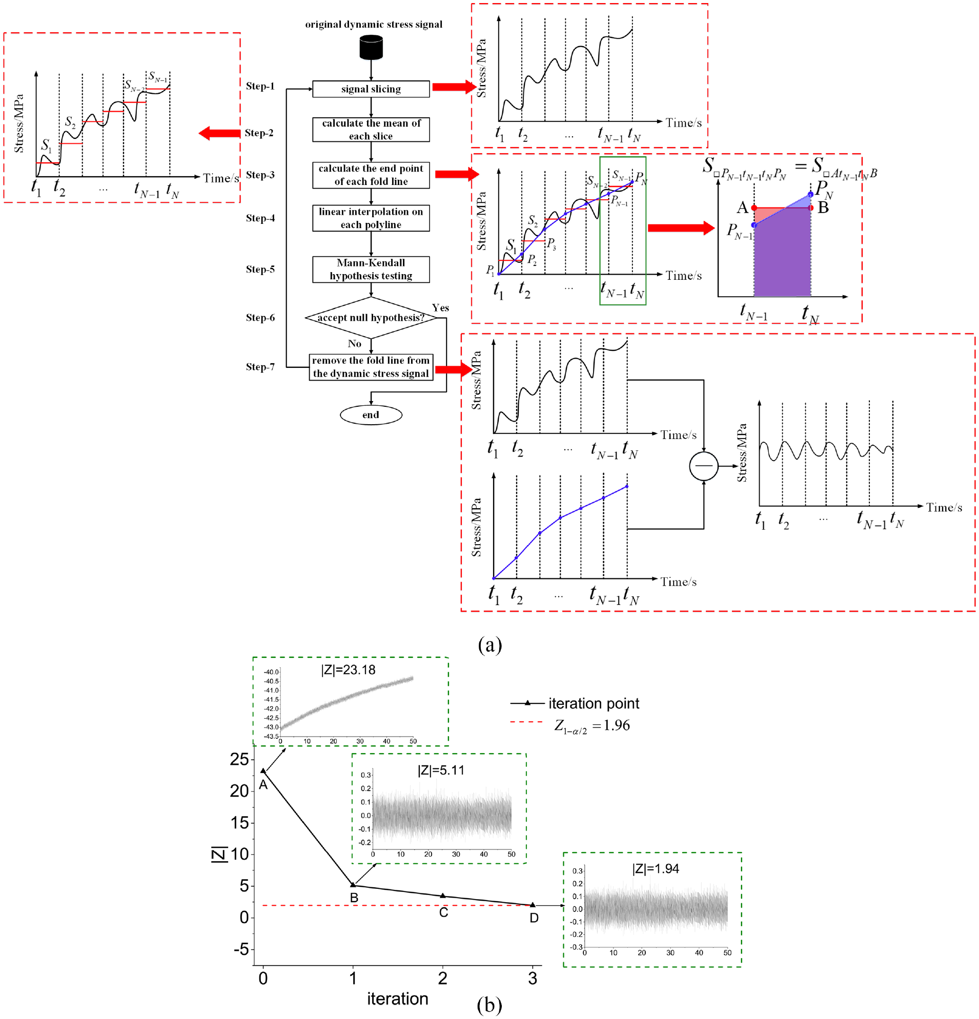
Trend removal method: (a) TRM calculation process, (b) TRM iterative process.

The TRM first slices the original signal of length $N$ and calculates the mean value $S_{k} (k = 1, 2, 3, \dots N - 1)$ of each slice, and then calculates the endpoint value $P_{i} (i = 1, 2, 3, \dots N)$ of the corresponding fold line for each slice based on the mean value of each slice, where:

P_{i} = {\begin{matrix} P_{1} & i = 1 \\ \frac{S_{i - 1} + S_{i}}{2} & i = 2, 3, \dots N - 1 \\ \frac{3 S_{N - 1}}{2} - \frac{S_{N - 2}}{2} & i = N \end{matrix}

(1)

In formula (1), $P_{1}$ is the value of the first point in the original signal.

Based on the linear drift assumption, the sequence of endpoint values is linearly interpolated to obtain a trend line of equal length to the original dynamic stress signal. A Mann-Kendall trend test was performed on the trend line to define the statistics $S_{t}$ defined as follows:

S_{t} = \sum_{k = 1}^{n - 1} \sum_{j = k + 1}^{n} sgn (x_{j} - x_{k})

(2)

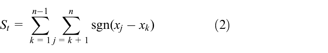
Where $sgn (x)$ is a symbolic function defined as follows:

sgn (x_{j} - x_{k}) = {\begin{matrix} 1 & x_{j} - x_{k} > 0 \\ 0 & x_{j} - x_{k} = 0 \\ - 1 & x_{j} - x_{k} < 0 \end{matrix}

(3)

Then the Mann-Kendall trend test statistic $Z$ is:

Z = {\begin{matrix} \frac{S_{t} - 1}{\sqrt{V ar (S_{t})}} & S_{t} > 0 \\ 0 & S_{t} = 0 \\ \frac{S_{t} + 1}{\sqrt{Var (S_{t})}} & S_{t} < 0 \end{matrix}

(4)

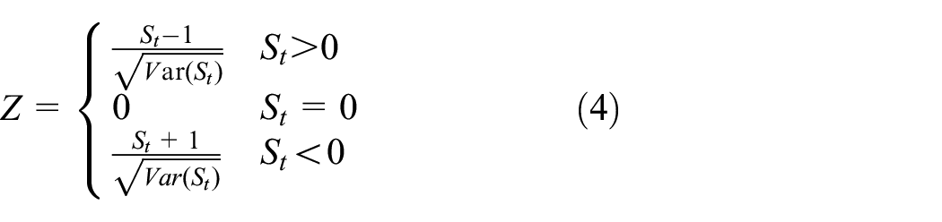
In formula (4), $Var (S_{t})$ is the variance of the statistic $S_{t}$ .

In the process, the iteration abort is determined as follows: at a given confidence level $α$ , if the null hypothesis is rejected, that is, $| Z | \geq Z_{1 - α / 2}$ , it means that there is still a trend term in the stress signal, at this time, the original signal is subtracted from the trend line point by point to get the dynamic stress signal after the removal of the trend line, and then the trend line of the dynamic stress signal is calculated again after the updating, and then the cycle is repeated until the Mann-Kendall test accepts the null hypothesis or the maximum number of iterations is exceeded, then the iteration is aborted.

Taking confidence level 95% as an example, at this time, $Z_{1 - α / 2} = 1.96$ , the iterative process of performing TRM is shown in Figure 1(b).

In Figure 1(b), point A represents the original dynamic stress signal, and point B to point D represent an iteration process. It can be seen that after performing three iterations using TRM, the zero-drift trend is completely removed.

Signal spike detection

Signal spike duration can be divided into two types, one is a short duration (within 10 ms) discrete spike, and the other is a long duration (within 0.2 s) continuous spike. For the above two types of signal spikes, the detection model proposed in this paper consists of two stages, as shown in Figure 2.

Figure 2.

Signal spike detection process.

Data transformation

Rolling weighted standard deviation is a statistical indicator used to calculate the volatility of a time series by introducing a weight coefficient and assigning higher weights to recent observations to effectively capture the impact of newer data on the overall volatility. The rolling weighted standard deviation is usually calculated using a sliding window, each window contains $N$ points, and the formula is as follows:

σ_{R} = \sqrt{\frac{1}{N} \frac{\sum_{i = 1}^{N} w_{i} {(x_{i} - \bar{x})}^{2}}{\sum_{i = 1}^{N} w_{i}}}

(5)

Where: $w_{i}$ is the weight coefficient, $\bar{x}$ is the weighted average, $x_{i} (i = 1, 2, 3, \dots N)$ is the point in the sliding window.

According to the weighted average definition, there is:

\bar{x} = \frac{\sum_{i = 1}^{N} w_{i} x_{i}}{\sum_{i = 1}^{N} w_{i}}

(6)

Substitute formula (6) into formula (5), there is:

σ_{R} = \sqrt{\frac{1}{N} \sum_{i = 1}^{N} w_{i} {x_{i}}^{2} - {\bar{x}}^{2}}

(7)

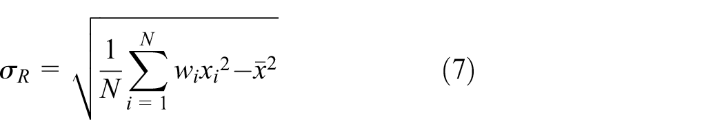
According to formula (7), the rolling weighted standard deviation is affected by the distribution of window length and weight coefficient, which are fixed and cannot be adjusted adaptively according to the signal spike duration. In this section, a recursive method for calculating the instantaneous rolling weighted standard deviation is proposed. The specific calculation steps are as follow.

Step 1. Define two initial weight coefficients $W_{0}$ and $W_{1}$ , where $W_{1} = 1 - W_{0}$ .

Step 2. Define the instantaneous weighted sum of squares $S_{W_{n}}^{2}$ and the instantaneous weighted mean ${\bar{X}}_{W_{n}}$ , there are:

S_{W_{n}}^{2} = {\begin{matrix} 0 & n = 0 \\ W_{0} S_{W_{n - 1}}^{2} + W_{1} {X_{n}}^{2} & n > 0 \end{matrix}

(8)

{\bar{X}}_{W_{n}} = {\begin{matrix} 0 & n = 0 \\ W_{0} {\bar{X}}_{W_{n - 1}} + W_{1} X_{n} & n > 0 \end{matrix}

(9)

Where: $X_{n}$ is the current calculated dynamic stress value, $n$ is the point number.

Step 3. Calculate the instantaneous rolling weighted standard deviation $σ_{I R_{n}}$ , there is:

σ_{I R_{n}} = \sqrt{| S_{W_{n}}^{2} - {\bar{X}}_{W_{n}}^{2} |}

(10)

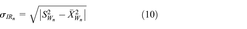
Define the residual contribution function $F (n)$ , there is:

F (n) = \frac{σ_{I R_{n}}}{σ_{I R_{1}}} \times 100 %

(11)

Substitute formula (10) into formula (11), there is:

F (n) = \sqrt{\frac{W_{0}^{n} (W_{0}^{n} - 1)}{W_{0} (W_{0} - 1)}}

(12)

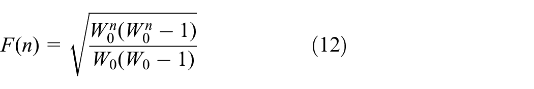
Take the derivative of formula (12), there is:

F' (n) = \frac{{W_{0}}^{n - 1} \ln W_{0} (2 {W_{0}}^{n} - 1)}{2 (W_{0} - 1) \sqrt{\frac{{W_{0}}^{n - 1} (W_{0}^{n} - 1)}{W_{0} - 1}}}

(13)

For any $n$ , in order to ensure that formula (13) is less than or equal to 0 constant, it is required that $W_{0}$ should be less than or equal to 0.5

Under different weight coefficients, the relationship between $F (n)$ and $n$ is shown in Figure 3(a).

Figure 3.

Data transformation: (a) residual contribution function with different initial weight coefficients, (b) minimum number of points with different initial weight coefficients, (c) comparison of computation time for different forms, (d) data transformation result.

When $W_{0} \leq 0.5$ , the residual contribution function is monotonically decreasing, and the closer $W_{0}$ is to 0, the higher the decay rate. When $W_{0} > 0.5$ , the residual contribution function first rises and then decays, and the closer $W_{0}$ is to 1, the lower the decay rate is.

The minimum number of calculation points required to decay the residual contribution function to 0.01% at $W_{0} \leq 0.5$ is shown in Figure 3(b).

With the increase of $W_{0}$ , the minimum number of points corresponding to the decay of the residual contribution function to below 0.01% increases gradually, taking $W_{0} = 0.05$ as an example, for a section of stable signal dynamic stress signal, after eight points, the IRWSD is only 0.0029% of the initial state, and after that, the IRWSD corresponding to all the points infinitely tends to be close to 0. If the point at a certain moment is a spike, the IRWSD will produce a sudden change due to the highest weight of the current calculation point, and the corresponding value is much larger than 0, thus effectively capturing the instantaneous fluctuation difference between the signal spike and the stable signal.

A comparison of the computation time of the rolling weighted standard deviation series based on the recursive form and based on the sliding window form is shown in Figure 3(c). As the scale of the data points of the sequence to be computed increases, the computation time of the recursive form is gradually shortened compared with that of the sliding window form, and the larger the scale of the data points is, the more obvious the improvement of computational efficiency is. Compared with the rolling weighted standard deviation in the form of sliding window, the algorithm complexity is reduced from $O (N)$ to $O (1)$ by using the recursive form, and its computation efficiency is greatly improved.

The original dynamic stress signal data transformation results are shown in Figure 3(d). Overall, the process of transforming the original dynamic stress signal into IRWSD contains a filtering effect, the effect of which is that the stable signals are suppressed to zero, while the non-stationary signals are enhanced, with the highest degree of enhancement at the point of the signal spike. Therefore, according to the final transformation result, the IRWSD sequences are divided into three regions, which are nonstationary spike region, nonstationary non-spike region, and stationary region.

Spike detection

Anomaly score sequence

Isolation forest is an unsupervised anomaly detection method proposed by Liu et al.³⁶ It is often used in anomaly detection tasks for large-scale data due to its linear time complexity and high accuracy.^32,34–36

When detecting outliers in isolation forests, it is considered that the population with sparse outlier distribution and high distance density is far away, and it is easiest to be separated in the process of multiple division. The anomaly score $S (x, n)$ is commonly used to represent the anomaly degree, and its formula is as follows:

{\begin{matrix} S (x, n) = 2^{- \frac{E (h (x))}{c (n)}}, n > 2 \\ c (n) = 2 H (n - 1) - \frac{2 (n - 1)}{n} \\ H (i) = \ln i + ξ \end{matrix}

(14)

In formula (14), $E (h (x))$ is the average path length of data $x$ in all isolation trees, $c (n)$ is the average path length of each isolation tree, and $n$ is the number of samples to build an isolation tree.

Normalization of the sequence of anomaly scores is available:

AS (x, n) = \frac{S (x, n) - min (S (x, n))}{max (S (x, n)) - min (S (x, n))}

(15)

To ensure randomness, $N_{F}$ isolation forests are constructed, and each forest contains $N_{T}$ isolation trees, then the result of the anomaly score sequence $A S_{k}$ of length $N$ is as follows:

{\begin{matrix} A S_{k} = \frac{\sum_{i = 1}^{N_{F}} A S_{i} (x, n)}{N_{F}} (k = 1, 2, \dots, N) \\ A S_{i} (x, n) = {A S_{i} (x_{1}, n), A S_{i} (x_{2}, n), S_{i} (x_{n}, n)} \end{matrix}

(16)

Anomaly score threshold

Typically, the anomaly score of non-spike points remains below 0.5. However, in some line sections, due to wheel-rail excitation like rail undulatory wear and wheel out-of-roundness, the excitation frequency coincides with the natural modal frequency of some structures of the bogie frame, leading to structural resonance. During this time, the dynamic stress response increases significantly, causing more violent signal fluctuations. Therefore, the threshold of anomaly score should be dynamically adjusted according to the signal fluctuation.

From a statistical point of view, the number of points corresponding to the non-spike regions is much larger than that of the spike regions, and if the anomaly score threshold is chosen reasonably, the cumulative probability of the anomaly score in the non-spike region should be much larger than that in the spike region, and the anomaly score threshold, that is, the anomaly score corresponding to a cumulative probability larger than a specified value. In order to determine the anomaly score cumulative distribution function (CDF), it is necessary to first calculate the probability density function (PDF) of the anomaly score.

To overcome the limitations of traditional parameter estimation methods, the kernel density estimation (KDE) method is used in this section to fit the IRWSD sequence distribution.

The probability density function ${\hat{f}}_{n} (x)$ is estimated as:

{\hat{f}}_{n} (x) = \frac{1}{Nh} \sum_{i = 1}^{n} K (\frac{x - xi}{h})

(17)

In formula (17), $h$ is the bandwidth coefficient, $N$ is the length of the anomaly score sequence, $K (•)$ is the kernel function, and the Gaussian kernel function is chosen, where:

K (x) = \frac{1}{\sqrt{2 π}} e^{- \frac{1}{2} x^{2}}

(18)

The bandwidth coefficient determines the accuracy of probability density estimation. In this section, the optimal bandwidth coefficient is calculated with the minimum of asymptotic mean integrated square error (AMISE) as the constraint condition, there is:

AMISE [\hat{f} (x)] = \frac{1}{nh} \int {K^{2} (u) du + \int [\frac{h^{2}}{2} f ″ (x) \int u^{2} K (u) du]}^{2} dx

(19)

u = \frac{x - x_{i}}{h}

(20)

Formula (19) is derived for $h$ and the derivative is taken to be zero to obtain the optimal bandwidth as:

\hat{h} = {\frac{{\int [K (u)]}^{2} du}{{[f ″ (x)]}^{2} dx {[\int u^{2} K (u) du]}^{2}}}^{\frac{1}{5}} n^{- \frac{1}{5}}

(21)

The kernel estimate of the cumulative distribution function is:

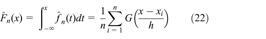
{\hat{F}}_{n} (x) = \int_{- \infty}^{x} {\hat{f}}_{n} (t) dt = \frac{1}{n} \sum_{i = 1}^{n} G (\frac{x - x_{i}}{h})

(22)

In formula (22), $G (x) = \int_{- \infty}^{x} K (t) dt$ .

Then, the anomaly score threshold is:

threshold = {\hat{F}}_{n}^{- 1} (x) |_{x = α}

(23)

In formula (23), ${\hat{F}}_{n}^{- 1} (x)$ represents the inverse function of the cumulative distribution function corresponding to the sequence of anomaly scores, and the value of any point of this function can be obtained by interpolating the cumulative probabilities after exchanging the cumulative probabilities with the coordinates of the anomaly scores, $α$ is the specified cumulative probability value.

Taking $α = 0.99$ as an example, using formula (24) to calculate the anomaly score threshold under different signal lengths, the results are shown in Figure 4.

Figure 4.

Anomaly score threshold under different signal lengths ( $α = 0.99$ ).

In Figure 4, it can be found that there are some differences in the CDF corresponding to different lengths of the anomaly score sequences, and the thresholds are adaptively adjusted according to the different signals to be detected. Among the anomaly score sequences of different lengths, the anomaly scores corresponding to spike regions are all above the threshold, while the anomaly scores corresponding to non-spike regions are all below the threshold except for very few points.

Experimental verification

Experimental dataset

The experimental measurement system is shown in Figure 5(a). The system mainly includes host computer, switch, data acquisition equipment and stress measurement point. Among them, each stress measurement point corresponds to a strain gauge, which is connected to a channel of the data acquisition system. At the same time, based on TCP/IP protocol, the collected data is sent to the host computer in real time by the switch for monitoring and analysis.

Figure 5.

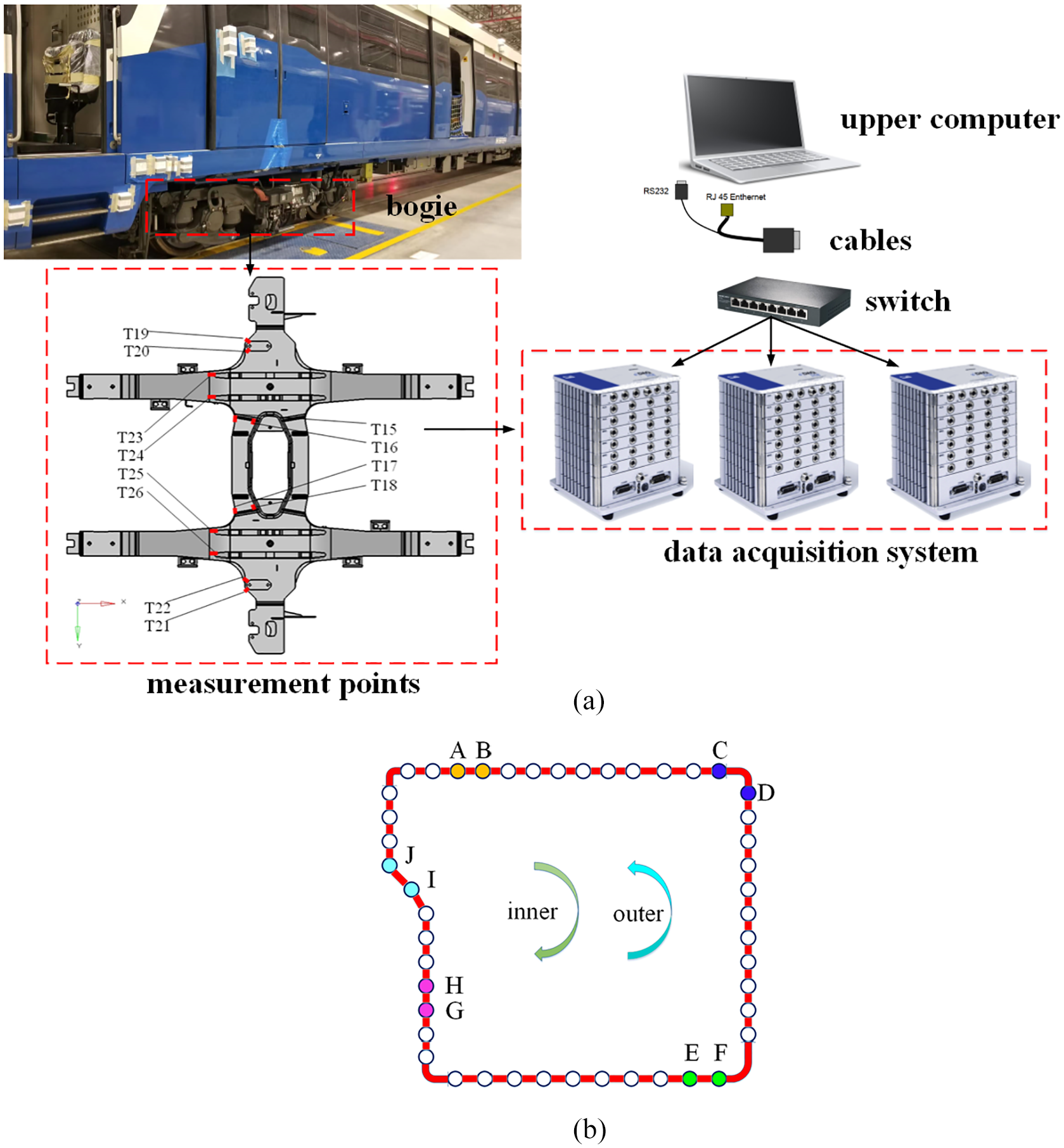
Metro dynamic stress experiment: (a) experimental measurement system, (b) experimental line schematic.

The experimental line schematic is shown in Figure 5(b), which includes an inner loop and an outer loop.

For the above experimental line, a 5-days experiment was carried out. It is statistically found that within the line sections A–B, C–D, E–F, G–H, and I–J, the signals of the measurement points in the different areas of the bogie frame contain more signal spikes, so this section constructs five datasets by the different dates of the experiment, and the detailed information is shown in Table 2.

Table 2.

Experimental detailed information.

Dataset name	Loop line	Line section	Measurement point number	Dataset sample size	Sample length(s)
DST_1	Outer	A–B/C–D/E–F/G–H	T1/T3/T5/T7/T9	20	10
DST_2	Inner	C–D/E–F/G–H/I–J	T12/T13/T23/T24/T25	20	10
DST_3	Outer	A–B/C–D/G–H/I–J	T2/T3/T4/T7/T10/T11	20	10
DST_4	Inner	C–D/E–F/G–H/I–J	T12/T13/T14/T26/T30	20	10
DST_5	Outer	A–B/E–F/G–H/I–J	T6/T8/T19/T22/T31	20	10

The dataset construction process involves manual labeling of each sample. This is done by slicing the samples at a length of 2 s and observing the anomalies within each slice. The anomalies are typically five times greater or more than the average value within the slice. If the duration of the anomalies is less than 0.2 s, all the points within 0.2 s are labeled as anomalies. On the other hand, if the duration is greater than 0.2 s, they are considered nonstationary non-spike signals and are left unlabeled.

Experimental evaluation indices

Spike detection rate

Spike detection rate (SDR) is used to evaluate the degree of overlap between algorithm detection results and manually labeled results in a continuous dynamic stress signal. When manual labeling results are presented as a continuous interval and algorithm detection results are given as discrete signal spike points, it becomes difficult to compare the two directly. To overcome this challenge, we have divided the sample into multiple detection units and treated the occurrence of a signal spike within a unit as a random event. In case a signal spike occurs within a unit, it is considered positive, and the position and frequency of the spikes are ignored. This paper sets the detection unit length to 0.2 s in combination with manual labeling rules.

Therefore, the SDR is calculated as follows.

Step 1. According to the start time $t_{1}$ and end time $t_{2}$ of the sample to be detected, the sample is divided into the detection unit set $TS = {T S_{1}, T S_{2}, T S_{3}, \dots T S_{n}}$ with $t_{s} = 0.2 s$ , which contains $n$ detection units, $n = (t_{2} - t_{1}) / t_{s}$ .

Step 2. Divide the manually labeled continuous interval to obtain the true positive detection unit set $T S_{AP}$ , where $T S_{AP} = {T S_{i}, T S_{i + 1}, \dots T S_{j}} \subseteq TS$ . In $T S_{AP}$ , $i = ⌊ (s t_{1} - t_{1}) / t_{s} ⌋ + 1$ , $j = ⌊ (s t_{2} - t_{1}) / t_{s} ⌋ + 1$ , $s t_{1}$ and $s t_{2}$ are the start time and end time of the manually labeled interval. The remaining intervals in the sample not labeled are defined as the true negative detection unit set $T S_{AN}$ , $T S_{AN} = ð_{TS} T S_{AP}$ .

Step 3. Calculate the detection units corresponding to the algorithm detection results point by point to form the predicted positive detection unit set $T S_{PP}$ , and the detection units corresponding to the points not labeled by the algorithm are defined as the predicted negative detection unit set $T S_{PN}$ , where $T S_{AN} = ð_{TS} T S_{AP}$ .

Step 4. Construct the confusion matrix according to $T S_{AP}$ , $T S_{AN}$ , $T S_{PP}$ , and $T S_{PN}$ , and define the number of detection units labeled as positive by the algorithm and manually as $TP$ , and the number of detection units labeled as negative as $TN$ . Thus, SDR is defined as:

SDR = \frac{TP + TN}{TP + TN + FP + FN} \times 100 %

(24)

Damage sensitivity

Damage sensitivity (DS) is used to evaluate the severity of signal spikes detected by the algorithm, and is described by the difference in structural damage before and after signal spike labeling and replacement. Ideally, the damage change based on algorithmic labeling and replacement should be consistent with the manual method, in which case the damage sensitivity is close to 1. When the algorithm is too severe, the damage sensitivity is less than 1. Conversely, damage sensitivity is greater than 1. The specific calculation process is as follows.

Step 1. Based on the simplified rainflow algorithm in the ASTM E1049-85 (2017) standard, the stress spectrum of 32-level blocks was constructed after rainflow counting of the pre-processing dynamic stress signals, and the Miner linear fatigue cumulative damage law combined with the parameters of S–N curves of the steel structures in BS EN 1993-1-9:2005 were used to calculate the damage corresponding to the current dynamic stress signals. The damage $D_{1}$ is:

D_{1} = \sum_{i = 1}^{32} \frac{n_{i} Δ {σ_{i}}^{m}}{Δ {σ_{C}}^{m} \times 2 \times 10^{6}}

(25)

In formula (25), $n_{i}$ represents the frequency of each spectrum block, $Δ σ_{i}$ represents the cycle range corresponding to each spectrum block, and $Δ σ_{C}$ represents the fatigue limit stress cycle range when the number of cycles is $2 \times 10^{6}$ . This paper takes 71 MPa as the value for $Δ σ_{C}$ . $m$ is the parameter of the S–N curve. In engineering practice, to leave a certain safety margin, the S–N curve without an inflection point is usually used, which means that $m$ is equal to 3.

Step 2. After labeling the signals, the points within the spike region are reconstructed. To prevent re-introducing a large range of stress cycles after reconstruction, the reconstruction region is first defined and then smoothed as shown in Figure 6.

Figure 6.

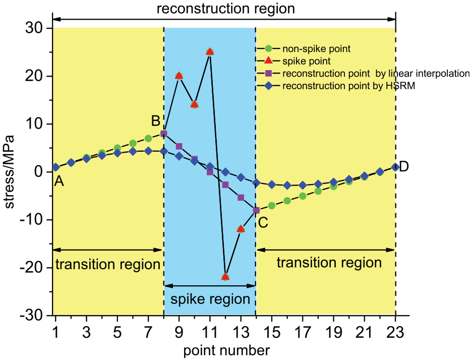
Signal spike reconstruction.

The reconstruction region contains two parts, namely the transition region and the spike region, in which the transition region is extended forward and backward according to the first and endpoints B and C of the spike region, respectively, until the first and endpoints A and D of the reconstruction region are equal, the transition region A–B and C–D are obtained.

To smooth the reconstruction region, the half-sine reconstruction method (HSRM) is established in this section, which removes the gradient discontinuity in the reconstruction region with the help of two half-sine functions, and the points within the reconstruction region are calculated as:

f (x_{i}) = A_{i} f_{1} (x_{i}) + B_{i} f_{2} (x_{i})

(26)

In formula (26), $A_{i} = {\underset{N_{1}}{\underset{︸}{t_{A B_{1}}, t_{A B_{2}}, \cdot t_{A B_{N_{1}}}}}, \underset{N_{2} + N_{3}}{\underset{︸}{t_{A B_{N_{1}}}, \cdot t_{A B_{N_{1}}}}}}$ , $B_{i} = {\underset{N_{1} + N_{2}}{\underset{︸}{t_{C D_{1}}, \cdot t_{C D_{1}}}}, \underset{N_{3}}{\underset{︸}{t_{C D_{1}}, t_{C D_{2}}, \dots t_{C D_{N_{3}}}}}}$ , $t_{A B_{i}}$ and $t_{C D_{i}}$ represent the values in the transition regions A–B and C–D, respectively. $N_{1}$ , $N_{2}$ , and $N_{3}$ , represent the lengths of the transition regions A–B, the spike region B–C, and the transition region C–D, respectively. $f_{1} (x)$ , $f_{2} (x)$ are the two half-sine functions, which are calculated as follows:

{\begin{matrix} f_{1} (x_{i}) = 0.5 + 0.5 \cos θ_{i} \\ f_{2} (x_{i}) = 0.5 - 0.5 \cos θ_{i} \\ θ_{i} = \frac{i - 1}{N - 1} π (i = 1, 2, 3, \dots N) \end{matrix}

(27)

In formula (27), $θ_{i}$ is the phase angle corresponding to each point in the reconstruction region, expressed in radians. $N$ is the total number of points in the reconstruction region, where $N = N_{1} + N_{2} + N_{3}$ .

In Figure 6, the reconstruction result using HSRM is smoother and introduces less stress cycle amplitude than the linear interpolation method.

Step 3. Calculate the damage value $D_{2}$ of the signal after reconstruction of the spike region in the same way as in Step 1.

Step 4. Define the damage sensitivity $DS$ as follows:

DS = \frac{S_{A}}{S_{M}}

(28)

In formula (28), $S_{A}$ is the damage residual obtained after detection and reconstruction using the method. $S_{M}$ is the damage residual obtained after using manual labeling and reconstruction. The damage residual $S$ is calculated as:

S = \frac{| D_{2} - D_{1} |}{D_{1}} \times 100 %

(29)

Discussions

The detection effects of different model parameters and detection algorithms were evaluated on five datasets, using spike detection rate and damage sensitivity as evaluation indices. The comparison results are shown in Figure 7.

Figure 7.

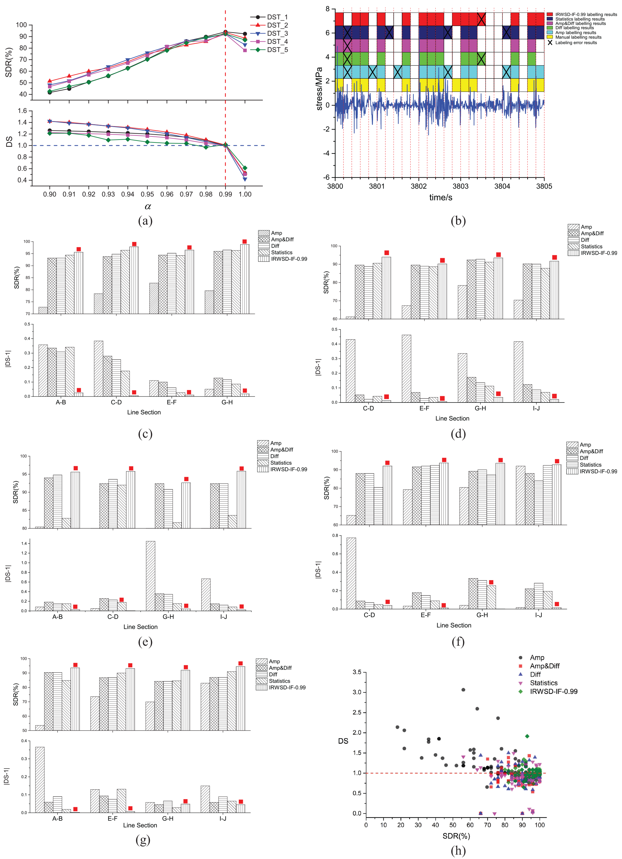
Experimental comparison results: (a) changes in evaluation indices at different values of $α$ , (b) different detection methods for labeling results, (c) comparison results in DST_1, (d) comparison results in DST_2, (e) comparison results in DST_3, (f) comparison results in DST_4, (g) comparison results in DST_5, (h) correlation between evaluation indices.

In Figure 7(a), the changes of SDR and DS of the detection model proposed in this paper are compared under different $α$ values. As $α$ increases, the SDR shows an increasing and then decreasing trend, in which when $α$ equals 0.99, the SDR takes the maximum value in different datasets. At the same time, DS shows a gradual decline, with $α$ less than 0.99, the decline is slower and greater than 1, and when $α$ is greater than 0.99, the SDR quickly decays below 1. In summary, 0.99 is the optimal value of $α$ .

Facing the large-scale task of dynamic stress signal spike detection for bogie frames, the four main methods in the literature⁴² are commonly used as the core methods. Take a sample in DST_1 as an example, the results of different methods’ labeling are shown in Figure 7(b).

In Figure 7(b), the length of each detection unit is 0.2 s. The labeling results reflect the ability of different methods to continuously determine the signal spikes in the time series, and through comparison, it is found that the labeling results of the detection model proposed in this paper are the most consistent with those of manual labeling.

The results of the comparison of the average SDR and DS for different line sections in each dataset are shown in Figure 7(c)–(g).

The results presented in Figure 7(c)–(g) demonstrate that the detection model proposed in this paper achieves the highest SDR in different line sections across the five datasets. Additionally, it has been found that the DS of this model is closest to 1 when compared to other methods. The results of different line sections in the same dataset have been averaged and are provided in Table 3.

Table 3.

Comparison of spike detection methods in different datasets.

Dataset name	SDR (%)					DS
Dataset name	Amp	Amp&Diff	Diff	Statistics	IRWSD-IF-0.99	Amp	Amp&Diff	Diff	Statistics	IRWSD-IF-0.99
DST_1	78.42	94.35	94.93	95.35	97.18	1.23	0.79	0.81	0.84	1.01
DST_2	70.34	90.46	90.17	90.01	92.34	1.41	0.90	0.93	0.96	0.99
DST_3	74.57	92.81	92.90	85.00	94.97	1.56	0.76	0.79	0.91	1.00
DST_4	79.29	89.25	88.53	88.10	93.04	1.22	0.79	0.80	0.88	1.02
DST_5	70.03	87.11	87.11	87.60	93.33	1.18	1.04	1.11	0.94	1.02
Average	74.53	90.80	90.80	89.21	94.17	1.32	0.86	0.89	0.91	1.01

In Table 3, in terms of the SDR, the average SDR of the five methods are 74.53%, 90.80%, 90.80%, 89.21%, and 94.17%, respectively, and the model proposed in this paper has the highest SDR. In terms of DS, the average values of the five methods in different datasets are 1.32, 0.86, 0.89, 0.91, and 1.01, respectively. Among them, the average DS of the method in this paper is the closest to 1. The results indicate superior generalization across line sections for the proposed model in this paper.

In Figure 7(h), a correlation can be observed between two indices. When the SDR is higher, the DS is closer to 1. A higher SDR means that more signal spike points are detected and labeled, consequently, the frequency distribution of the stress spectrum block of rainflow counts after these spike points have been reconstructed is closer to the manual labeling process. Furthermore, when both detection methods have the same SDR, it means that the number of times and positions of the labels are the same in the same number of detection units, however, it is essential to measure the exact number of correctly labeled spike points in each detection unit with the help of the DS index.

In addition, the results of the comparison of the total computation time of different algorithms in each dataset are shown in Figure 8(a)–(e).

Figure 8.

Comparison of the total computation time of different algorithms in each dataset, (a) comparison results in DST_1, (b) comparison results in DST_2, (c) comparison results in DST_3, (d) comparison results in DST_4, (e) comparison results in DST_5.

According to Figure 8(a)–(e), the total computation time of the model proposed in this paper is basically minimized in all the above five datasets. Among them, the evaluation indices are more time-consuming to compute compared to other datasets because DST_5 contains the most manual labeling results. On this dataset, the performance difference between the model proposed in this paper and the other models is the most obvious, and the efficiency is improved by about 16.7% compared with the other models, which indicates that the efficiency of spike detection and evaluation can be improved through the recursive complexity reduction and the acceleration of the linear time complexity of the isolation forest algorithm.

However, it should be pointed out that although the model proposed in this paper has a significant improvement in computation efficiency and spike detection accuracy compared to existing methods, the start point of the detection model kernel is the isolation forest algorithm. When the training samples contain a relatively dense signal spike, it will lead to deviations in the computation of the anomaly scores of the points, which will affect the distribution of the sequence of anomaly scores. In this case, the threshold needs to be optimized and adjusted again, and there is a certain degree of decline in computation efficiency. In addition, in the process of large-scale signal spike detection, the construction of isolation forests requires the establishment of a large number of iTrees, which is very easy to be limited by the maximum memory. Therefore, in future research work, we can take the lead in establishing a high-dimensional feature library of typical signal spikes and forming an apriori knowledge, use the apriori knowledge to correct the results of anomaly score computation, and at the same time, adopt incremental learning to construct and adjust the isolation forest, to reduce the computational resources and memory consumption.

Conclusions

This paper addresses the issue of signal spike detection in the dynamic stress monitoring of bogie frames. To solve this problem, a signal spike detection model based on isolation forest is proposed in this paper. The model effectively enhances the efficiency of signal spike detection and the accuracy of structural damage calculation.

In the data pre-processing stage, for the zero-drift problem in the original signal, this paper proposes a trend removal method (TRM) based on the assumption of segmented linear drift, which does not introduce signal oscillations, quantitatively describes the degree of zero drift, and combines iterative abort conditions to realize adaptive removal of zero-drift components.

In the signal spike detection stage, utilizing the difference between the instantaneous fluctuations of the signal spike region and the non-spike region, the IRWSD calculation in recursive form is proposed, which, combined with the monotonicity determination of the residual contribution function, effectively separates the signal spike region when the initial weight coefficients are less than or equal to 0.5, and at the same time, reduces the algorithm complexity from $O (N)$ to $O (1)$ . Based on the isolation forest, the normalized anomaly scores at each point of the IRWSD sequence are calculated, and the KDE method is used to adaptively determine the threshold. The results show that anomaly detection is optimal when the cumulative probability is 0.99.

Two indices, spike detection rate, and damage sensitivity, are constructed for evaluating the quality of signal spike detection. In the process, the half-sine reconstruction method (HSRM) is proposed to reconstruct the spike region, which has a continuous gradient and does not reintroduce a wide range of stress cycles compared to linear interpolation.

Finally, five datasets are constructed to compare the different detection methods with the field experimental data, and the results show that, compared with the existing methods, the detection model proposed in this paper improves the SDR by an average of 7.86%, and the DS by an average of 15.59%, which effectively improves the detection efficiency of the signal spikes, and ensures the accuracy of the subsequent structural damage evaluation.

Footnotes

Acknowledgements

The authors would appreciate the anonymous reviewers and the editor for their valuable comments.

Handling Editor: Tiago Alexandre Narciso da Silva

Declaration of conflicting interests

The author(s) declared no potential conflicts of interest with respect to the research, authorship, and/or publication of this article.

Funding

The author(s) disclosed receipt of the following financial support for the research, authorship, and/or publication of this article: This research was supported by National Natural Science Foundation of China (No. 62277001, 61877002) and China Academy of Railway Sciences Fund Project (No. 2022YJ145).

ORCID iD

Guang Wei Zhao

References

Yan

Jin

Sun

, et al. Active monitoring of fatigue crack in the weld zone of bogie frames using ultrasonic guided waves. Sensors 2019; 19: 1–13.

Wang

Ren

, et al. Improving the fatigue reliability of metro vehicle bogie frame based on load spectrum. Int J Fatigue 2020; 132: 1–13.

Lin

Liu

Chang

YW.

An investigation of the temperature-drift effect on strain measurement of concrete beams. Appl Sci (Basel) 2019; 9: 1–13.

Feng

Cao

ZH.

Analysis and research on electromagnetic compatibility of high speed railway traction current harmonics to track circuit. IEEE Trans Appl Supercond 2021; 31: 1–4.

Wen

Wang

, et al. A network-based method to analyze EMI events of on-board signaling system in railway. Appl Sci (Basel) 2020; 10: 1–18.

Bellan

Spadacini

Fedeli

, et al. Space-frequency analysis and experimental measurement of magnetic field emissions radiated by high-speed railway systems. IEEE Trans Electromagn Compat 2013; 55: 1031–1042.

Chandola

Banerjee

Kumar

Anomaly detection: a survey. ACM Comput Surv 2009; 41: 1–58.

Salgado

Azevedo

Proença

, et al. Noise versus outliers. In: MIT Critical Data (ed.) Secondary analysis of electronic health records. Cham: Springer, 2016, pp.163–183.

Grubbs

FE.

Procedures for detecting outlying observations in samples. Technometrics 1969; 11: 1–21.

10.

Wilson

Emerson

Spike detection: a review and comparison of algorithms. Clin Neurophysiol 2002; 113: 1873–1881.

11.

Velis

DR.

Stochastic sparse-spike deconvolution. Geophysics 2008; 73: R1–R9.

12.

Sapiro

Mallat

Solving inverse problems with piecewise linear estimators: from Gaussian mixture models to structured sparsity. IEEE Trans Image Process 2012; 21: 2481–2499.

13.

Yan

Sun

A non-negative Bayesian learning method for impact force reconstruction. J Sound Vib 2019; 457: 354–367.

14.

Liu

Qiao

Wang

, et al. Non-convex sparse regularization via convex optimization for impact force identification. Mech Syst Signal Process 2023; 191: 17.

15.

Miller

Ghalyan

Mondal

, et al. HMM conditional-likelihood based change detection with strict delay tolerance. Mech Syst Signal Process 2021; 147: 1–17.

16.

Xiong

Yan

Qin

, et al. Quantitative assessment of the impact of extreme events on electricity consumption. Energies 2024; 17: 1–18.

17.

Zhou

Tang

. Continuous anomaly detection in satellite image time series based on z-scores of season-trend model residuals. In: 36th IEEE international geoscience and remote sensing symposium (IGARSS), 2016, pp.3410–3413. Beijing, Peoples R China: IEEE.

18.

Yan

Chronopoulos

Yuen

, et al. Structural anomaly detection based on probabilistic distance measures of transmissibility function and statistical threshold selection scheme. Mech Syst Signal Process 2022; 162: 1–22.

19.

Soriano-Vargas

Werneck

Moura

, et al. A visual analytics approach to anomaly detection in hydrocarbon reservoir time series data. J Pet Sci Eng 2021; 206: 1–15.

20.

Chen

Jiang

Yan

, et al. Dynamic warning method for structural health monitoring data based on ARIMA: case study of Hong Kong-Zhuhai-Macao bridge immersed tunnel. Sensors 2022; 22: 1–17.

21.

Chu

. Iterative anomaly detection algorithm based on time series analysis. In: 15th IEEE international conference on mobile ad hoc and sensor systems (MASS), 2018, pp.548–552. Chengdu, Peoples R China: IEEE.

22.

Wang

Real-time defect detection of high-speed train wheels by using Bayesian forecasting and dynamic model. Mech Syst Signal Process 2020; 139: 1–15.

23.

Zhu

, et al. Time series outlier detection based on sliding window prediction. Math Probl Eng 2014; 2014: 1–14.

24.

Zhu

Liu

, et al. Anomaly detection and multi-step estimation based remaining useful life prediction for rolling element bearings. Mech Syst Signal Process 2024; 206: 1–28.

25.

Liu

Gryllias

A semi-supervised support vector data description-based fault detection method for rolling element bearings based on cyclic spectral analysis. Mech Syst Signal Process 2020; 140: 1–24.

26.

Sarmadi

Karamodin

A novel anomaly detection method based on adaptive Mahalanobis-squared distance and one-class kNN rule for structural health monitoring under environmental effects. Mech Syst Signal Process 2020; 140: 1–24.

27.

Zhao

XJ.

POD: a parallel outlier detection algorithm using weighted kNN. IEEE Access 2021; 9: 81765–81777.

28.

Entezami

Sarmadi

Behkamal

A novel double-hybrid learning method for modal frequency-based damage assessment of bridge structures under different environmental variation patterns. Mech Syst Signal Process 2023; 201: 1–22.

29.

Qais

Kewat

Loo

, et al. Early outlier detection in three-phase induction heating systems using clustering algorithms. Ain Shams Eng J 2024; 15: 1–14.

30.

Nonclercq

Foulon

Verheulpen

, et al. Cluster-based spike detection algorithm adapts to interpatient and intrapatient variation in spike morphology. J Neurosc Methods 2012; 210: 259–265.

31.

Riahi-Madvar

Nasersharif

Azirani

. Subspace outlier detection in high dimensional data using ensemble of PCA-based subspaces. In: 26th international computer conference of the Computer-Society-of-Iran, Tehran, Iran, 3–4 March 2021, pp.1–5. IEEE.

32.

Shao

, et al. Cluster-based improved isolation forest. Entropy 2022; 24: 1–17.

33.

Zhang

Tang

Yang

RJ.

Data anomaly detection for structural health monitoring by multi-view representation based on local binary patterns. Measurement 2022; 202: 1–12.

34.

Hariri

Kind

Brunner

RJ.

Extended isolation forest. IEEE Trans Knowl Data Eng 2021; 33: 1479–1489.

35.

Karczmarek

Kiersztyn

Pedrycz

Fuzzy set-based isolation forest. In: IEEE international conference on fuzzy systems (FUZZ-IEEE), Glasgow, UK, 19–24 July 2020, pp.1–6. IEEE, 2020.

36.

Liu

Ting

Zhou

ZH.

Isolation-based anomaly detection. ACM Trans Knowl Discov Data 2012; 6: 1–39.

37.

Gong

Feng

. A novel deep learning approach for anomaly detection of time series data. Sci Program 2021; 2021: 1–11.

38.

Jin

, et al. Detecting unexpected faults of high-speed train bogie based on Bayesian deep learning. IEEE Trans Veh Technol 2021; 70: 158–172.

39.

Sbarufatti

Manes

Giglio

Performance optimization of a diagnostic system based upon a simulated strain field for fatigue damage characterization. Mech Syst Signal Process 2013; 40: 667–690.

40.

Klarák

Andok

Malik

, et al. From anomaly detection to defect classification. Sensors 2024; 24: 1–14.

41.

Kang

Chen

Wang

, et al. A new dual-input deep anomaly detection method for early faults warning of rolling bearings. Sensors 2023; 23: 1–13.

42.

Limited HUK. Spike detection. In: Glyph reference guide. Darmstadt, Germany: HBM Corporation Limited, 2015, pp.528–538.

A novel spike detection model for dynamic stress monitoring of bogie frame

Abstract

Keywords

Introduction

Data pre-processing

Signal spike detection

Data transformation

Spike detection

Anomaly score sequence

Anomaly score threshold

Experimental verification

Experimental dataset

Experimental evaluation indices

Spike detection rate

Damage sensitivity

Discussions

Conclusions

Footnotes

Acknowledgements

Declaration of conflicting interests

Funding

ORCID iD

References