New methods and applications of structural dynamics modeling for railway freight liquid tank

Abstract

As railway freight technology advances towards heavy-load, high-speed capabilities, the design of liquid tank products is evolving to prioritize high load capacity, lightweight, high-strength materials, low structural rigidity, and thin-walled construction. These changes result in pronounced nonlinear low-frequency vibrations during rail operation. Addressing these complex liquid-solid coupled vibrations requires accurate dynamic modeling of the structural system. This paper introduces a novel dynamic modeling method for liquid tank products based on acousto-elastic coupling. This approach considers the swaying of the free liquid surface and liquid-solid interactions, enabling precise characterization of these dynamics in a unified model. Specifically, it tackles the challenge of uneven node swaying forces caused by non-uniform liquid surface meshing, presenting a technique and program to adjust swaying recovery forces based on nodes’ actual coverage area. This method’s liquid sway frequency calculations showed a 10% precision increase over traditional methods, more accurately reflecting liquid vibration states. The paper applies these techniques to a single tank container and an LNG tank container on a flatbed trailer. Through theoretical, simulation, and experimental comparisons, the model’s accuracy and reasonableness were validated. This low-dimensionality, high-precision dynamic model is universally applicable, especially valuable in modeling complex engineering structures.

Introduction

With the development of railway freight technology, the operation speed of tank containers has increased to 220 km/h and the load of liquid cargo has increased, necessitating a tank container structure that is lighter, thinner, and stronger. This leads to a decrease in structural frequency, making the liquid sloshing frequency approach that of the tank container structure, thereby enhancing the liquid-solid coupling effects. ¹ During operation, the mass effect of the liquid varies, making dynamic simulation a challenge. The coupling of liquid sloshing and structural vibrations can lead to system instability, increase the risk of overturning, and impose additional dynamic loads. If vibrations couple with the main frequency, it may lead to structural fatigue failure. ² Therefore, a comprehensive assessment of the dynamic characteristics of liquid tank containers is crucial for product design.

Studies on the dynamic characteristics of liquid tank containers are sparse. NASA, combining modal tests of filled tanks, has developed a spring-mass model for filled tanks that takes into account the circumferential stiffness of the tank and the longitudinal stiffness of the liquid. ³ Tang et al., ⁴ based on the traditional lateral and torsional vibration one-dimensional beam model, has integrated a longitudinal spring-mass model, enabling the simultaneous calculation of lateral, longitudinal, and torsional modes and their coupled modes, thus improving the accuracy of frequency calculations in each direction.

The study methods for liquid sloshing primarily include experimental, analytical, and numerical approaches.^5,6 Although experimental methods are highly reliable, they are costly and have poor reproducibility, especially in the study of coupled dynamics in liquid tank containers. Analytical methods generally rely on the conservation laws of fluid motion, establishing approximate mathematical models of fluid motion to address the issue of liquid sloshing, but are often limited to simple, regular-shaped tanks. Early research utilized potential flow theory to establish theoretical models for minor liquid sloshing in regularly shaped tanks. ⁷ Subsequently, the multi-dimensional modal analysis method proposed by Faltinsen et al.^8–10 became the most commonly used analytical method for studying non-linear liquid sloshing. Compared to the former methods, numerical methods are deemed most suitable for studying liquid sloshing due to their flexibility and intuitiveness. This approach mainly involves computational fluid dynamics, which has seen the development of various spatial discretization techniques over the decades, such as finite difference methods, finite volume methods, finite element methods, and boundary element methods. ¹¹ The numerical methods for liquid modeling primarily include the lumped mass method, virtual mass method, and liquid rod element method. ¹² Although the virtual mass method more closely approximates the actual dynamics of liquids and improves computational accuracy, it generates a full mass matrix of the same scale as the degrees of freedom at the tank and liquid interface, which requires significant computational effort and struggles to simulate the effects of free surface sloshing.^13–15 While CFD methods, ALE methods, or CEL numerical analysis techniques can address issues like sloshing frequency, mass, and damping within tanks,^16–18 they typically only provide the modal shape of the liquid surface or partial sloshing parameters, and they struggle to comprehensively consider the coupling effects between sloshing and structure. Additionally, the accurate simulation of sloshing recovery forces is crucial for obtaining precise frequencies and modal shapes, yet there remains a lack of reliable modeling methods to achieve high-precision sloshing characteristics.^19,20

From existing research on the dynamics of liquid-solid coupling in liquid tank containers, it is evident that most studies focus primarily on either liquid sloshing or structural vibrations, with insufficient comprehensive consideration of the coupling effects. There is still a lack of precise and reliable modeling methods to simulate the recovery forces of sloshing, which limits the high-precision understanding of liquid sloshing characteristics. Current studies (as referenced in Wang et al., ¹⁶ Zhu et al., ¹⁷ Akkerman et al., ¹⁸ Sezen et al., ¹⁹ and Deng et al. ²⁰ ) usually focus only on the modal shapes of the liquid surface or certain sloshing parameters, and there is a relative lack of comprehensive analysis of the coupling effects between sloshing and structure. Although various experimental, analytical, and numerical methods have been employed to study the dynamic characteristics of liquid tank containers, there is still a lack of a comprehensive assessment method to fully consider the dynamic responses of liquid tank containers in aspects such as vertical, lateral, torsional, and sloshing movements. Therefore, this research further explores the establishment of theoretical models, improvement of numerical simulation methods, and experimental validation. Firstly, a finite element formulation suitable for the dynamic characteristics of liquid-solid coupling in large liquid tank containers was derived. For the calculation of sloshing characteristic parameters of the free liquid surface inside the tank, a method and corresponding program were proposed to correct the sloshing recovery force based on the actual coverage area of the free liquid surface grid nodes, which were validated through a simple tank case. Finally, using this modeling method and program, the liquid-solid coupling characteristics and liquid sloshing properties of LNG tank containers were studied and validated through a liquid-solid coupling modal test, establishing a set of dynamic calculation methods that comprehensively consider both liquid-solid coupling effects and liquid sloshing effects in liquid tank containers. This provides significant support for the establishment of dynamic models of liquid-solid coupling in complex engineering structures and the design and development of liquid tank containers.

The establishment of liquid-solid coupled dynamic equations

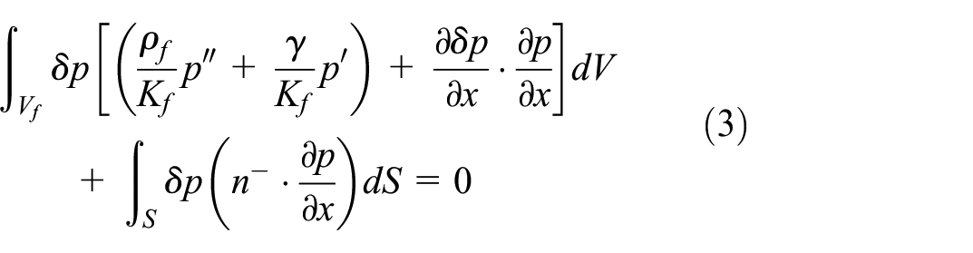
For a compressible, inviscid, and small perturbation fluid, the equations governing the motion within the liquid domain, expressed in terms of pressure, are as follows:

$$\frac{{\rho }_f}{K_f}p″+\frac{\gamma }{K_f}p\prime -\frac{\partial }{\partial x}·\left(\frac{\partial p}{\partial x}\right)=0$$

(1)

Where, $p$ represents the dynamic pressure of the liquid, $x$ denotes the spatial coordinates of a liquid particle, ${\rho }_f$ is the density of the liquid, $\gamma$ represents the force per unit volume due to the velocity, and $K_f$ stands for the bulk modulus of the liquid. The equivalent weak form of equation (1) can be expressed as:

$${\int }_{V_f}\delta p[\frac{{\rho }_f}{K_f}p″+\frac{\gamma }{K_f}p\prime -\frac{\partial }{\partial \mathit{x}}·\left(\frac{\partial p}{\partial \mathit{x}}\right)]\mathrm{dV}=0$$

(2)

Performing integration by parts on equation (2), we obtain:

$$\begin{array}{c}{\int }_{V_f}\delta p[(\frac{{\rho }_f}{K_f}p″+\frac{\gamma }{K_f}p\prime )+\frac{\partial \delta p}{\partial x}·\frac{\partial p}{\partial x}]\mathrm{dV}\hfill \\ +{\int }_S\delta p(n^{-}·\frac{\partial p}{\partial x})\mathrm{dS}=0\hfill \end{array}$$

(3)

The boundary conditions for the liquid domain can be classified into two categories: the free surface of the liquid (denoted as $S_f$ ) and the interface between the solid and the liquid (denoted as $S_{\mathrm{fs}}$ ), with their respective governing equations as follows:

$$\{\begin{array}{c}\frac{\partial p}{\partial z}=-\frac{1}{g}\frac{{\partial }^{2}p}{\partial t^2}\hfill \\ \frac{\partial p}{\partial n}=-{\rho }_f{a}_n\hfill \\ {\sigma }_{\mathrm{ij}}{n}_{\mathrm{sj}}=p{n}_{\mathrm{si}}\hfill \end{array}\begin{array}{c}\mathrm{on}{S}_f\hfill \\ \multicolumn{1}{c}{\mathrm{on}{S}_{\mathrm{fs}}}\end{array}$$

(4)

Where, g is the gravitational acceleration, ${\rho }_f$ is the density of the liquid, and $a_n$ is the normal acceleration of the solid domain wall. ²¹

When the liquid undergoes small amplitude oscillations, there should be no separation phenomenon at the interface between the liquid and the container. Therefore, the displacements, velocities, and accelerations along the normal direction of the liquid-structure interface should remain consistent with those of the container wall along the boundary. The variational form of the equations governing the liquid domain can be rewritten as:

$$\begin{array}{c}{\int }_{V_f}\delta p[(\frac{{\rho }_f}{K_f}p″+\frac{\gamma }{K_f}p\prime )+\frac{\partial \delta p}{\partial x}·\frac{\partial p}{\partial x}]\mathrm{dV}\hfill \\ -{\int }_{S_f}\delta p(\frac{\partial p}{\partial n}+\frac{1}{g}p″)\mathrm{dS}-{\int }_{S_{\mathrm{fs}}}\delta p(\frac{\partial p}{\partial n}+{\rho }_f{a}_n)\mathrm{dS}=0\hfill \end{array}$$

(5)

If the solid domain satisfies the displacement boundary conditions of the structure, it can be expressed as:

$$\begin{array}{c}{\int }_{V_s}\delta u_i({\sigma }_{\mathrm{ij},j}+f_i-{\rho }_s{u}_i\prime \prime )\mathrm{dV}-{\int }_{S_{\sigma }}\delta u_i({\sigma }_{\mathrm{ij}}{n}_{\mathrm{sj}}-{\overline{T}}_i)\mathrm{dS}\hfill \\ -{\int }_{S_{\mathrm{fs}}}\delta u_i({\sigma }_{\mathrm{ij}}{n}_{\mathrm{sj}}+p{n}_{\mathrm{sj}})\mathrm{dS}=0\hfill \end{array}$$

(6)

Integrating equation (6) by parts and substituting into the physical equation yields:

$$\begin{array}{c}{\int }_{V_s}[\delta {\epsilon }_{\mathrm{ij}}{D}_{\mathrm{ijkl}}{\epsilon }_{\mathrm{kl}}-f_i+\delta u_i({\rho }_s{u}_i\prime \prime +\mu u_i\prime )]\mathrm{dV}\hfill \\ -{\int }_{S_{\sigma }}\delta u_i{\overline{T}}_i\mathrm{dS}+{\int }_{S_{\mathrm{fs}}}\delta u_i\left(p{n}_{\mathrm{si}}\right)\mathrm{dS}=0\hfill \end{array}$$

(7)

Where, ${\sigma }_{\mathrm{ij}}$ represents the solid stress components, $u_i$ represents the solid displacement components, $f_i$ is the solid volume force components, is the solid mass density, $\mu$ is the damping coefficient, and ${\overline{T}}_i$ and $u_i$ are the known force components and displacement components, respectively, on the solid boundaries. ²²

The pressure field in the liquid domain and the displacement field in the solid domain are discretized using the finite element method. The pressure in the liquid domain elements is represented using nodal pressures and shape functions, while the displacement in the solid domain elements is represented using nodal displacements and shape functions as follows:

$$p(x,y,z,t)=\sum _{i=1}^{m_f}{N}_i(x,y,z)p_i(t)=N{\mathit{p}}^e$$

(8)

$$u\left(x,y,z,t\right)=\sum _{i=1}^{m_s}{\overline{N}}_i(x,y,z)u_i(t)=\overline{N}{\mathit{u}}^e$$

(9)

Where, $m_f$ and $m_s$ are the numbers of nodes within the liquid and solid elements, respectively; ${\mathit{p}}^e$ is the nodal pressure vector for the solid elements; ${\mathit{u}}^e$ is the nodal displacement vector for the liquid elements; $N_i$ and ${\overline{N}}_i$ are the interpolation functions for the corresponding nodes. ²³

Substituting equations (8) into (5) and (9) into (7), and considering the arbitrariness of $\delta p$ and $\delta u_i$ , the finite element equations for the fluid-structure coupled system can be obtained as follows:

$$\begin{array}{c}\left[\begin{array}{cc}{M}_s\hfill & 0\hfill \\ \multicolumn{1}{c}{-Q^T}& M_f\hfill \end{array}\right]\left[\begin{array}{c}\mathit{u}″\hfill \\ \multicolumn{1}{c}{\mathit{p}″}\end{array}\right]+\left[\begin{array}{cc}{C}_s\hfill & 0\hfill \\ \multicolumn{1}{c}{0}& C_f\hfill \end{array}\right]\left[\begin{array}{c}\mathit{u}\prime \hfill \\ \multicolumn{1}{c}{\mathit{p}\prime }\end{array}\right]\hfill \\ +\left[\begin{array}{cc}{K}_s\hfill & \frac{1}{{\rho }_f}Q\hfill \\ \multicolumn{1}{c}{0}& K_f\hfill \end{array}\right]\left[\begin{array}{c}\mathit{u}\hfill \\ \multicolumn{1}{c}{\mathit{p}}\end{array}\right]=\left[\begin{array}{c}{\mathit{F}}_s\hfill \\ \multicolumn{1}{c}{0}\end{array}\right]\hfill \end{array}$$

(10)

Where, $\mathit{p}$ is the nodal pressure vector for the liquid; $\mathit{u}$ is the nodal displacement vector for the solid structure; $Q$ is the fluid-structure coupling matrix; $M_f$ and $K_f$ are the liquid mass and stiffness matrices, respectively; $M_s$ and $K_s$ are the solid mass and stiffness matrices, respectively; $M_s$ and $K_s$ are the structural and fluid damping matrices, respectively; ${\mathit{F}}_s$ is the external load vector on the solid structure. ²⁴

The mass matrices, stiffness matrices, damping matrices, and external load vectors for the liquid and solid domains are assembled from their respective sets of elements, with each element’s parameter expressions given as follows:

$$\begin{array}{cc}\multicolumn{1}{c}{M_f}& =\sum _e{M}_f^e=\sum _e{\int }_{V_f^e}\frac{{\rho }_f}{K_f}{N}^T\mathrm{NdV}+{\int }_{S_f^e}\frac{1}{g}{N}^T\mathrm{NdS}\hfill \\ \multicolumn{1}{c}{K_f}& =\sum _e{K}_f^e=\sum _e{\int }_{V_f^e}\frac{\partial N^T}{\partial x_i}\frac{\partial N}{\partial x_i}\mathrm{dV}\hfill \\ \multicolumn{1}{c}{M_s}& =\sum _e{M}_s^e=\sum _e{\int }_{V_s^e}{\rho }_s{\overline{N}}^T\mathrm{NdV}\hfill \\ \multicolumn{1}{c}{K_s}& =\sum _e{K}_s^e=\sum _e{\int }_{V_s^e}{B}^T\mathrm{DBdV}\hfill \\ \multicolumn{1}{c}{C_f}& =\sum _e{C}_f^e=\sum _e{\int }_{V_f^e}\frac{\gamma }{K_f}{N}^T\mathrm{NdV}\hfill \\ \multicolumn{1}{c}{C_s}& =\sum _e{C}_s^e=\sum _e{\int }_{V_s^e}\mu {\overline{N}}^T\mathrm{NdV}\hfill \\ \multicolumn{1}{c}{Q^e}& =\sum _e{Q}^e=\sum _e{\int }_{S_{\mathrm{fs}}^e}{\rho }_f{\overline{N}}^T{n}_s\mathrm{NdV}\hfill \\ \multicolumn{1}{c}{F_s}& =\sum _e{F}_s^e=\sum _e{\int }_{V_f^e}{\overline{N}}^T\mathrm{fdV}+{\int }_{S_{\sigma }^e}{\rho }_s{\overline{N}}^T\overline{N}\mathrm{dS}\hfill \end{array}$$

(11)

Where, $B$ is the displacement-strain relationship matrix for the solid domain, typically composed of two parts, namely:

$$M_f^e=M_{\mathrm{fV}}^e+M_{\mathrm{fS}}^e$$

(12)

Where, $M_{\mathrm{fV}}^e$ is the mass matrix induced by the compressibility of the liquid; $M_{\mathrm{fS}}^e$ is the mass matrix induced by the free surface wave fluctuations of the liquid.

For ease of solving the general eigenvalue problem, the equation is manipulated by setting external loads to zero, yielding:

$$\left[\begin{array}{cc}{\overline{M}}_s\hfill & E\hfill \\ \multicolumn{1}{c}{E^T}& {\overline{M}}_f\hfill \end{array}\right]\left[\begin{array}{c}\mathit{u}″\hfill \\ \multicolumn{1}{c}{\mathit{p}″}\end{array}\right]+\left[\begin{array}{cc}{\overline{K}}_s\hfill & E\hfill \\ \multicolumn{1}{c}{E^T}& {\overline{K}}_f\hfill \end{array}\right]\left[\begin{array}{c}\mathit{u}\hfill \\ \multicolumn{1}{c}{\mathit{p}}\end{array}\right]=\left[\begin{array}{c}0\hfill \\ \multicolumn{1}{c}{0}\end{array}\right]$$

(13)

Where, ${\overline{M}}_s=M_s+1/{\rho }_{f}Q{K}_f^{-1}{Q}^T$ , ${\overline{M}}_f=1/{\rho }_f{M}_f{K}_f^{-1}{M}_f$ , ${\overline{K}}_s=K_s$ , $E=-1/{\rho }_f{\mathrm{QK}}_f^{-1}{M}_f$ , and ${\overline{K}}_f=1/{\rho }_f{K}_f$ ; the dynamic characteristic equation of the system can be obtained as:

$$(\left[\begin{array}{cc}{\overline{K}}_s\hfill & E\hfill \\ \multicolumn{1}{c}{E^T}& {\overline{K}}_f\hfill \end{array}\right]-{\omega }^2\left[\begin{array}{cc}{\overline{M}}_s\hfill & E\hfill \\ \multicolumn{1}{c}{E^T}& {\overline{M}}_f\hfill \end{array}\right])\left[\begin{array}{c}\mathit{u}\hfill \\ \multicolumn{1}{c}{\mathit{p}}\end{array}\right]=\left[\begin{array}{c}0\hfill \\ \multicolumn{1}{c}{0}\end{array}\right]$$

(14)

According to the obtained coefficient matrix, which is a symmetric banded sparse matrix, general algorithms for solving large-scale eigenvalue problems can be employed to address the eigenvalue problem of fluid-structure coupling. ²⁵

Development of a liquid oscillation model program

There are three main methods for addressing the characteristics of liquid sloshing in engineering: theoretical calculations, numerical analysis, and experimental testing. Theoretical calculation methods are only suitable for cases with simple and regular liquid surfaces or for approximating complex liquid surface shapes to simpler forms, resulting in lower accuracy and limited applicability in engineering. Experimental testing methods face limitations due to experimental conditions and environments, making it challenging to conduct tests, especially for closed and opaque containers. Currently, in engineering practice, the solution to liquid sloshing characteristics often involves the use of finite element modeling through software. However, due to constraints imposed by the liquid surface mesh, it is difficult to accurately calculate the restoring forces during liquid sloshing, impacting the assessment of parameters related to liquid sloshing characteristics.

Recognizing the importance of liquid sloshing characteristics in engineering and the limitations of existing methods for addressing sloshing issues, this study integrates MATLAB with ABAQUS software calculation files. This integration harnesses the programming capabilities of MATLAB and the computational power of ABAQUS. The MATLAB program is designed to call ABAQUS calculation results files, enabling a comprehensive analysis of liquid sloshing characteristics.

Establishment of oscillation model

Neglecting the damping at the liquid surface, by combining the fluid-structure coupling equations with the boundary conditions of the free liquid surface, the expression for the liquid sloshing equation is obtained as ²⁶ :

$$\begin{array}{c}{M}_f\mathit{p}″+K_f\mathit{p}=0\hfill \\ \frac{\partial p}{\partial z}=-\frac{1}{g}\frac{{\partial }^{2}p}{\partial t^2}\begin{array}{c}\mathrm{on}{S}_f\hfill \end{array}\hfill \end{array}$$

(15)

The above equation is an eigenvalue problem related to pressure. Solving the combined equations yields the expression for the restoring force during liquid sloshing as:

$$F_{\mathrm{fluid}\mathrm{restoring}\mathrm{force}}=\rho \mathrm{gA}$$

(16)

Where, $\rho$ is the liquid density, $g$ is the gravitational acceleration, and $A$ represents the differential area of the free liquid surface.

In order to characterize the oscillation modes of the free surface, it is necessary to attach a layer of membrane elements on the free surface. Since membrane elements only have in-plane stiffness and zero out-of-plane stiffness, they can precisely depict the oscillation patterns of the free surface. Additionally, during the free liquid surface oscillation, each differential area of the free liquid surface experiences a restoring force generated by an overload (or gravity). Taking the magnitude of the restoring force as the stiffness of spring elements provides the restoring force for the oscillation of the liquid surface.^27,28 In a regular grid (see Figure 1), each node covers the same area, making it easy to determine the restoring force for each node. However, in practical engineering problems, the liquid surface is a complex and irregular interface. When dividing the grid, it is not possible to obtain equal-sized face meshes for each node, resulting in unequal restoring forces for each node. Therefore, a universal method is needed to handle the situation of irregular grids (as shown in Figure 2).

Figure 1.

Regular grid liquid surface.

Figure 2.

Irregular grid liquid surface.

For irregular liquid surfaces, this paper proposes the approach illustrated in Figure 3, employing a structured grid for the meshing of the liquid surface. In this approach, each element has four nodes. Therefore, the liquid area covered by node $i$ can be approximated as one-fourth of the sum of the areas shared by $n$ elements using that node. The formula for calculating the area is as follows:

$$A_i=\frac{1}{4}(A_1+···+A_n)$$

(17)

Where, $A_1$ to $A_n$ an represent the areas of elements 1 through $n$ , which can be directly calculated from the coordinates of the four nodes. ²⁹

$$\begin{array}{c}A=\sqrt{(p-a)(p-b)(p-c)(p-d)}\hfill \\ p=(a+b+c+d)/2\hfill \end{array}$$

(18)

Where, $a$ , $b$ , $c$ , and $d$ represent the lengths of the four sides of the mesh element. Based on the method proposed in this paper, batch processing can be applied to the mesh membrane elements and nodes, providing accurate restoring forces for each mesh node, thereby enhancing the accuracy of solving liquid sloshing characteristics.

Figure 3.

Methods for handling irregular liquid surfaces.

Figure 4.

Computational analysis workflow based on ABAQUS and MATLAB software.

Development of liquid sloshing program

To meet the computational requirements of fluid-structure coupling dynamics, a fluid-structure coupling finite element model is established in ABAQUS software. The model includes mesh elements, material properties, boundary conditions, and connection settings. The properties of the liquid surface mesh element are defined as membrane elements. Two sets, named “FREE_SURFACE_ELEMENT_SET” and “FREE_SURFACE_NODE_SET,” are created for the liquid surface mesh elements and nodes, respectively, to facilitate data retrieval in MATLAB. Contact connections between the free liquid surface membrane elements and the liquid elements are established using the TIE contact. To simulate the restoring force on the liquid surface, spring elements are employed, and SPRING elements are created by selecting nodes of the free liquid surface mesh elements. The SPRING elements are initialized and assigned values. The modal analysis step is set up without performing the computational analysis, and the INP file is generated for output.

Using the “XLS_READ” function in MATLAB, the data for the free liquid surface elements and nodes are extracted from the INP file based on the specified keywords. A “FOR” loop is employed to read the element and node IDs of the free liquid surface membrane elements. The “FIND” function is then applied to locate the positions of the four node IDs composing each element in the node set. The row and column data constituting the nodes of each element are stored in a matrix, and the spatial coordinates of the nodes are obtained by indexing the node column data using the node IDs. The area of each element is calculated using the Heron’s formula (18). Next, the “FIND” function is used to determine the number of elements shared by each node and their corresponding element IDs. An “IF_ELSE IF” selection statement is utilized to categorize the cases based on the shared element count. Formulas (17) and (18) are then applied to calculate the restoring forces for each node. The “FOPEN” function is used to open the INP file generated by ABAQUS software. A “FOR” loop and “FPRINTF” function are employed to rewrite the restoring forces for each node into the INP file in the format specified under the “*SPRINT” keyword. The modified INP file is then submitted to ABAQUS software for computational analysis, followed by post-processing of the results.

Application examples

Application example on single tank

In this case study, a single tank structure consists of two parts: the cylindrical section and the two end caps. The cylindrical section has a length (L) of 10 m and a wall thickness of 2 mm. The two end caps are ellipsoidal, with a major axis (a) of 1.414 m and a minor axis (b) of 1.0 m. The bottom end cap has a thickness of 2 mm, while the top end cap has a thickness of 4 mm. The material properties of the tank structure include an elastic modulus (E) of 70 GPa, a Poisson’s ratio of 0.333, and a density of 7.85 × 10³ kg/m³. The liquid level inside the tank is 10 m (measured from the juncture of the cylindrical section and the bottom). The liquid properties include a density of 1 × 10³ kg/m³, a speed of sound of 1435 m/s, and a gravitational acceleration of 9.8 m/s ² . It is assumed that the tank structure is elastic and the liquid is an ideal fluid, which is non-viscous, incompressible, and irrotational.

The theoretical solution for the natural frequency of liquid sloshing in the circular tank is given by the following formula ³⁰ :

$$w_i=\sqrt{{\lambda }_i\frac{g}{a}\left(\tan H\right)\left({\lambda }_i\frac{H}{a}\right)}$$

(19)

Where, $w_i$ is the $i$ order frequency of liquid sloshing, and ${\lambda }_i$ is the $i$ root of the first-order Bessel function derivative.

Based on the above parameters, a finite element model of the tank container is established. The liquid domain inside the tank is simulated using acoustic elements, with the element type being AC3D8. AC3D8 is a linear eight-node hexahedral element, with three displacement degrees of freedom per node. The total number of elements is 20,956. The free surface of the liquid inside the tank is simulated using membrane elements, with the element type being M3D4. M3D4 is a four-node quadrilateral element, with three degrees of freedom (displacement degrees of freedom) per node. This element is used to simulate in-plane stress and strain in membranes, without considering bending stiffness. The total number of elements is 284. The structural domain of the tank body is simulated using shell elements, with the element type being S8R5. S8R5 is an eight-node quadrilateral shell element with quadratic shape functions. Each node has 6 degrees of freedom (3 translational degrees of freedom and 3 rotational degrees of freedom), which can accurately simulate the real behavior of shell structures. The total number of elements is 5128. For the fluid-structure interaction, a contact pair is created to connect the liquid and structural domains. The mesh surface of the liquid domain is designated as the “slave surface,” with the outward facing surface being the positive direction. Similarly, the mesh surface of the structural domain is designated as the “master surface,” with the inward facing surface being the positive direction. These surfaces are constrained and connected using TIE contact pairs. Material properties are assigned separately to the solid and liquid domains. The hyperelastic material parameters for the membrane elements at the liquid’s free surface are as indicated in the referenced literature. ³¹ The liquid sloshing restoring force is applied using both the equal restoring force method and the method proposed in this paper for computational analysis. Figure 5 shows the computational model of the tank container; To reduce the solution time and ensure rapid convergence, the Lanczos method is employed for modal analysis of a single tank; Figure 6 shows the results of the modal calculation for the liquid-solid coupled modes in a single tank. From the figure, it is evident that the primary vibration modes of the tank under liquid-solid coupling are longitudinal vibrations along the tank body and lateral vibrations perpendicular to the tank body. The first row in the figure represents the modal shapes of longitudinal vibrations, and the second row represents the modal shapes of lateral vibrations perpendicular to the tank. It can also be observed from the figure that the vibration forms at the top and bottom of the tank differ; this is mainly because the top of the tank is not affected by the liquid, whereas the vibration form at the bottom is the result of liquid-structure coupling.

Figure 5.

Parameters of the single tank calculation model: (a) geometric dimensions, (b) liquid model, and (c) structural model.

Figure 6.

Vibrational modes of liquid-solid coupling in tank structure.

The frequencies of the first five modes of liquid sloshing, calculated using the formula (20) for the frequencies of liquid sloshing on the free surface of cylindrical tanks, are listed in Table 1. The methods proposed in this paper and those from Jia et al. ³² were also applied to analyze the sloshing modes of the liquid inside the tank, with Figure 7 displaying the first five sloshing modes. Table 1 lists the calculated results and comparisons of the frequencies of liquid surface sloshing within the tank, where m and n respectively represent the numbers of half-waves in two mutually perpendicular directions on the liquid free surface. As can be seen from Table 1, the sloshing frequencies calculated using the restoring force correction method and procedure proposed in this paper are consistent with the analytical solutions. Without correcting the sloshing restoring force and applying the same restoring force to each node, the calculated frequency results show a significant error compared to the analytical solutions. Additionally, the sloshing mode shapes (see the second row of Figure 7) exhibit obvious singularities due to excessively high local restoring forces. The modal shapes obtained using the method described in Jia et al. ³² are similar to those in the second row of Figure 7 because the correction for nodal sloshing recovery forces was not considered.

Table 1.

Comparison of calculated frequencies for liquid sloshing in the tank (unit: rad/s).

Parameter	Modal vibration mode order
	1	2	3	4	5
(m,n)	(0,1)	(1,1)	(2,2)	(2,1)	(3,0)
${\lambda }_i$	1.426	1.841	4.201	3.054	4.806
Theoretical solution	0.501	0.534	0.654	0.694	0.746
Methodology and results of this study	0.556	0.579	0.701	0.755	0.801
Error (%)	10.97	8.43	7.19	8.79	7.37
Methodology and results of reference	0.507	0.537	0.655	0.688	0.744
Error (%)	1.20	0.56	0.15	−0.09	−0.27

Figure 7.

Free surface liquid sloshing mode shape in a tank.

Application example on flatbed trailer with LNG tank container

Modal analysis using acousto-elastic coupling method

The modal test was conducted on a 40-foot LNG (liquefied natural gas) tank container (47.2 m ³ tank container) mounted on a shared flatcar of type NX70A. The modal analysis under the liquid-solid coupling effects of the “flatcar + LNG tank container” was performed using the acoustic-solid coupling method. The structural components were primarily simulated using shell elements, and the material properties of the main components are presented in Table 2.

Table 2.

Material properties of major components.

Name	Material	Elastic modulus (GPa)	Poisson’s ratio
Container, piping, interlayer piping, external piping	06Cr19Ni10	200	0.3
Outer container cylinder head	16MnDR	206	0.3
Outer cylinder reinforcement ring, skirt ring	Q355NE	200	0.3
Corner posts, end bottom braces, side bottom braces	Q450NQR1	210	0.3
Remaining frame components	SPA-H	210	0.3
Inner container support	Fiberglass D3848	30	0.25
Outer container epoxy fiberglass support cover	16MnDII	206	0.3

In practical operations, the flatcar and the tank container are connected via corner seats. In building the computational model, an equivalent simplification is made, with the actual connections simplified to RBE3 element connections. The lateral and longitudinal degrees of freedom at the main nodes of the RBE3 elements at the four corner seats are constrained, while the vertical degrees of freedom are released to meet the equivalent constraints of the actual conditions. Figure 8 shows the liquid-solid coupling analysis model for the “flatcar + LNG tank container” and the equivalent connection diagram at the corner seats. To verify the accuracy of the method proposed in the paper and the reliability of the program, a condition with a 75% fill level was selected for calculation and analysis. This allows for an effective comparison and validation of the calculation results with the experimental results. To ensure the liquid fill level is 75% of the total tank volume, the closed liquid domain was segmented and its volume calculated using the meshing software (Hypermesh). After confirming the closed liquid domain volume to be 35.4 m ³ , the liquid domain was meshed. The fluid domain was simulated using water, and the free surface of the liquid inside the tank was simulated using membrane elements, with the element type being M3D4. The liquid portion is modeled using AC3D8 elements, and the part of the container in contact with the liquid is simulated using S8R5 elements. In the areas where the liquid contacts the solid and the free liquid surface contacts the liquid, TIE contact pairs are established for constraint connections. The connection between the flatcar and the bogie is equivalently modeled as a spring element, with the spring element stiffness parameter at the center plate connection being 4000 N/mm and at the side bearing connection being 2200 N/mm. The restoring force on the liquid’s free surface is applied using the calculation method and procedure proposed in this paper. The INP file is executed for solving, and the Lorenz method is employed to extract the first 20 modal parameters of the model. Figure 9 presents the typical modal calculation results under the liquid-solid coupling of the “flatcar + LNG tank container”; the yawing mode shape, rolling mode shape, and pitching mode shape represent the rigid-body motion modes of the “flatcar + LNG tank container.” The first order bending mode shape frequency under the coupling of the LNG tank container and the flatcar is 13.73 Hz, the coupling frequency of the flatcar torsion mode shape and the LNG tank container breathing mode shape is 17.18 Hz, and the frequency of the first order vertical bending mode shape of the LNG tank container side beams is 23.36 Hz. Figure 10 shows the typical sloshing modal calculation results for the liquid inside the tank; from the contour maps of the modal shape calculation results, it can be seen that the liquid inside the tank vibrates in two mutually perpendicular directions on the free surface. There are mainly three types of vibration forms: vibrations along one vertical direction (as shown in (a) and (b) of Figure 10); vibrations along another vertical direction (as shown in (c) of Figure 10); and coupled vibrations along two perpendicular directions (as shown in (d), (e), and (f) of Figure 10). At lower frequencies, the liquid primarily vibrates along one vertical direction; as the frequency increases, the coupled vibrations in two perpendicular directions become more intense. In the contour map of the sloshing mode shape, areas in blue represent regions with smaller vibration amplitudes, while areas approaching red indicate regions with increasingly larger vibration amplitudes.

Figure 8.

Analysis model and equivalent connections on flatbed trailer with LNG tank container.

Figure 9.

Modal vibration modes of the liquid-solid coupling on flatbed trailer with LNG tank container: (a) yaw mode shape, (b) roll mode shape, (c) pitch mode shape, (d) opposite bending mode shape, (e) flatcar torsion and tank breathing mode shape, and (f) first order vertical bending mode shape of side beam.

Figure 10.

Sloshing mode shapes of liquid inside the tank: (a) liquid lateral second order wave motion, (b), liquid lateral third order wave motion, (c) liquid longitudinal second order wave motion, (d) liquid longitudinal three-zone wave motion, (e) liquid longitudinal six-zone wave motion, and (f) liquid longitudinal multi-zone wave motion.

Modal test based on full-scale railway freight car vibration test rig

Modal tests for the “flatcar + LNG tank container” under liquid-solid coupling were conducted using the railway freight car body fatigue and whole vehicle vibration test rig. Before the experiment, fill the tank with water and use the level sensor to ensure the fill level is 75%. The test rig system comprises three parts: a test rig excitation system, a data acquisition system, and a modal analysis system. The basic schematic of the modal test is shown in Figure 11(a). Figure 11(b) shows the ongoing modal test for the “flatcar + LNG tank container.”

Figure 11.

Liquid-solid coupling modal test on flatbed trailer with LNG tank container: (a) test system block diagram and (b) LNG tank container field physical testing.

Test vehicle excitation: The vehicle in its ready-to-operate state is placed on the four wheel pair support beams of the test rig, with one end of the vehicle connected to the test rig via a hinged device, and the other end remaining unhinged and free. Two vertical actuators are connected under each wheel pair support beam, and one lateral actuator is connected at one end of the support beam. The actuators excite the vehicle in vertical and lateral vibrations through the wheel pair support beams. The vehicle’s natural frequencies are tested using a random method, with the frequency range of the test rig excitation system being 0.4–40 Hz.

Sensor layout: Vertical and lateral acceleration sensors are deployed at both ends and the midsection of the flatcar, with sensor IDs NX_11, NX_12, NX_21, NX_22, NX_13, and NX_23, totaling 12 acceleration sensors, as shown in Figure 12. Acceleration sensors are also positioned on the eight corner pieces of the tank container, identified as A1–A4 and B1–B4. Each measurement point is equipped with both vertical and lateral acceleration sensors, totaling 16 acceleration sensors. At the central ends of the cylinder, two measurement points, A5 and B5, are each equipped with vertical, lateral, and longitudinal acceleration sensors, totaling six acceleration sensors. Additionally, two vertical acceleration measurement points, C1 and C2, are set up on the two support seats at the center of the tank body. A schematic of the tank container acceleration sensor placement is shown in Figure 12. After completing the sensor installation, the data acquisition equipment is connected, and the sampling frequency of the acquisition device is set to 521 Hz. Using LMS Test.Lab software, the test vehicle model is built, and various test parameters are set to conduct the modal test.

Figure 12.

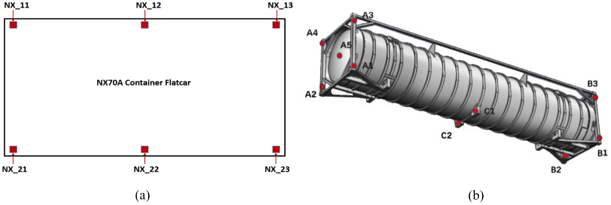
Schematic diagram of acceleration sensor layout for modal test: (a) acceleration sensor layout on NX70A container flatcar and (b) LNG tank container acceleration sensor layout.

Analysis of the test modes: Operational Modal Analysis (OMA) is employed to analyze the results of the modal test. The frequency response function is obtained by dividing the cross-spectral density function of the acceleration response and excitation force by the autospectral density function of the excitation force. The PolyMAX method is used for modal parameter identification. This method, particularly effective in the presence of strong damping and dense modes, allows for a clear depiction of the steady-state diagram, thus facilitating the physical mode order determination, and providing the modal frequencies, shapes, and damping ratios of the vehicle body. ³³ The results of the experimental modal parameter identification are shown in Table 3.

Table 3.

Modal test results on flatbed trailer with LNG tank container.

Modal order	Mode shape description	Frequency (Hz)	Damping ratio (%)
First order mode shape	Yaw mode shape	5.73	16.12
Second order mode shape	Roll mode shape	9.07	2.42
Third order mode shape	Pitch mode shape	14.04	8.63
Fourth order mode shape	Flatcar and tank container reverse bending	15.03	4.06
Fifth order mode shape	First order vertical bending of side beam	23.51	0.21
Sixth order mode shape	Flatcar torsion and tank container breathing	17.73	6.83

Results comparison and analysis

To further verify the effectiveness of the algorithm proposed in this paper, the calculated modal results on flatbed trailer with LNG tank container are compared with the experimental modal results, and the comparison is shown in Table 4. The modeling method presented in this paper can simultaneously obtain the lateral, vertical, and torsional modal results on flatbed trailer with LNG tank container, as well as the sloshing modal results of the liquid inside the tank. The comparison of the calculated results with the experimental results shows that the maximum error in the frequencies of yaw, roll, and pitch modes is 10.12%. This is mainly due to the simplification of the model during the modal analysis, where the nonlinear connection between the bogie and the body is equivalently treated as a spring connection, neglecting the effect of the coupled modes between the bogie and the body, leading to certain comparative errors. However, the frequency error of the elastic body modes of the flatcar and tank container is relatively small. This is mainly because the influence of the liquid mass and stiffness, as well as the mutual coupling between the liquid in the tank and the tank container, are considered in the calculation. These results indicate that the modeling method proposed in this paper can provide high computational accuracy and meet the requirements of engineering applications.

Table 4.

Comparison of primary frequencies (unit: Hz).

Mode shape description	Modal test results	Modal calculation result	Error (%)
Yaw mode shape	5.73	5.15	−10.12
Roll mode shape	9.07	8.81	−2.87
Pitch mode shape	14.04	14.83	5.63
Flatcar and tank container reverse bending	15.03	13.73	−8.65
First order vertical bending of side beam	23.51	23.36	−0.63
Flatcar torsion and tank container breathing	17.73	17.18	−3.11

Conclusion

This paper derives the finite element formulation of the equations for liquid-solid coupled dynamics, proposes a method based on correcting the liquid sway recovery force according to the actual covered area of the mesh nodes, and develops a program that integrates the capabilities of ABAQUS and MATLAB software, addressing the issue of low calculation and analysis precision in analyzing complex liquid surface sway characteristics. Applied to two typical engineering examples, through comparative analysis of theoretical simulation and experimental results, the following conclusions are drawn:

• (1) The dynamic modeling method proposed in this paper is applied to analyze the vibration modes of circular tank containers. Compared to the method using equal recovery forces, there is a significant improvement in the accuracy of identifying liquid sloshing frequencies and mode shapes, about 10%. This indicates that the improved method effectively enhances the analysis capability for sloshing mode shape singularity issues and the analytical precision of sloshing frequencies, thereby validating the correctness of the coupled system numerical simulation method presented in this paper.

• (2) The method was applied to simulate the sloshing of the free liquid surface and the liquid-solid coupling effects in a “flatbed trailer and LNG tank container” system. It was found that there is a strong coupling phenomenon between the tank container structure and the liquid cargo. The sloshing of the liquid cargo has a significant impact on the entire structural system that cannot be ignored. Accurate modeling and prediction of liquid cargo sloshing are crucial for the precision of the dynamic analysis of the structural system.

• (3) This method can identify parameters that cannot be calculated by theoretical analysis methods, and can also supplement results unattainable by experimental methods. It possesses both the versatility and applicability to solve similar engineering problems. As the objects of engineering applications become increasingly complex, the use of the dynamic analysis method presented in this paper to predict engineering models demonstrates potential advantages.

• (4) Limitations of the study: despite the achievements of this study, there are some limitations: The simplification process in the model, where the nonlinear connection between the bogie and the body is treated as a spring connection, neglects the effect of the coupled modes between the bogie and the body, leading to certain comparative errors. Moreover, the current model has not yet fully considered the impact of the liquid’s dynamic response under extreme operational conditions, such as during high-speed operation or abrupt track changes. Future research will aim to improve these limitations and explore more combinations of experimental validation and theoretical models to enhance the accuracy and applicability of the model.