Sage Journals: Discover world-class research

Abstract

Tank vehicles have quite poor roll stability in driving. Therefore, the purpose of this article is to investigate tankers’ roll stability by vehicle dynamic modeling. As a fluid–solid coupling multi-body system, tank vehicle’s dynamic modeling must take liquid sloshing into account. The conventional solution on liquid sloshing by hydrodynamics is difficult and time-consuming, and the modeling of tankers obtained by this method was a distributed parameter system with infinite degree of freedoms. It was quite difficult and complicated to analyze tankers’ dynamic features and to design active control system by the distributed parameter system. Therefore, three different methods to describe liquid sloshing effects in partially filled tanks with elliptical cross sections were proposed in this article, which are the estimation of liquid sloshing, the improved estimation of liquid sloshing, and the modeling of equivalent mechanical model for liquid sloshing. Then, the dynamic modeling of tank vehicles was commenced based on that. It was found out that the roll stability performance of tank vehicles obtained by different models differs with each other. The quasi-static model obtained by the estimation of liquid sloshing could get an estimation on tanker’s rollover threshold quickly and easily, but it is with poor accuracy. The improved quasi-static model obtianed by the improved estimation of liquid sloshing could give a more accurate result on tanker’s rollover threshold, the solution is also easily and quickly. Rollover analysis based on equivalent mechanical model of liquid sloshing could reflect vehicle’s dynamics and is with high accuracy, but the process is of great complexity.

Keywords

Tank vehicles roll stability liquid sloshing dynamic modeling of tank vehicles the estimation of liquid sloshing equivalent mechanical model for liquid sloshing

Introduction

Road tank vehicles are commonly used in carrying a wide range of liquid cargoes, mainly of a dangerous nature, such as chemical and petroleum products. Statistical analysis showed that there were nearly 80% of global chemical products delivered by tank vehicles, and the transportation freight had already reached 4 billion tons per year. However, tankers also create severe traffic safety problems, which would result in huge people injury and property damage. Statistical data collected by Statistique Canada had shown that 83% of lorry rollover accidents on highways are caused by tankers.¹ A US study had reported that the average annual number of tanker rollovers is about 1265, which accounts for 36.2% of the total number of heavy vehicle highway accidents.² In 2011, there were 416 tanker accidents occurred in China, which resulting in more than 400 people being injured or killed, as well as immense economic losses. Besides those, the release of fluid cargo often happens in tanker accidents, which would cause environment contamination.³ Therefore, great attention must be paid to tanker driving safety.

Much works had been carried out on the features of tanker accidents. It was found out by Treichel et al.⁴ that rollover is the main type in tanker accidents, and it accounts for 45% of the total tanker accidents. At the same time, rollovers for ordinary trucks only account for 4% of the total truck accidents. Many research efforts had been made to investigate factors behind this phenomenon, and it was universally accepted that liquid sloshing in partially filled tanks is the most important one.^5,6 Due to the limitation on tank filling percentage, tanks are partially filled with fluid cargo most of the time. Thereafter, the changing of vehicle driving state brings into liquid sloshing.^7,8 As a result, lateral sloshing force acting on the tank wall increases rollover torque and degrades vehicle roll stability.

Different from ordinary truck, tank vehicle is a complicated fluid–solid coupling multi-body system. Liquid sloshing and vehicle driving interact with each other, the modeling of tank vehicles must take the dynamic characteristics of liquid sloshing into consideration. Therefore, the study on liquid sloshing dynamics is of great significance. Until now, many efforts had been made, and the main methods to investigate liquid sloshing dynamics can be summarized as follows:

Hydrodynamic analysis. Linear liquid sloshing for uncompressible ideal fluid with small amplitudes was usually described by potential flow theory. Linear theory was used to solve governing equations, so as to obtain sloshing frequency and mode. Thereafter, the forced sloshing could be studied, and sloshing force and torque would also be calculated. Results obtained by this method were quite accurate. However, only liquid sloshing in a few tanks could be solved using this method.^9–11

The computational fluid dynamics (CFD) method. Sloshing parameters can also be acquired by solving governing equations based on Navier–Stokes equation directly. While the analytical solution to nonlinear partial differential equations was quite difficult, numerical solution was utilized and carried out on computer. The CFD is suitable in most cases.^12,13

The experimental method. By test platform or tank vehicles, liquid sloshing can be observed and relevant parameters be monitored by reproducing liquid sloshing.^14,15 Simulation software was also used to simulate liquid sloshing and to obtain the dynamic effects.^16,17

Based on the study on liquid sloshing dynamics, many researches on the modeling of fluid–solid coupling system had been carried out. By now, subjects mainly focus on liquid-filled spacecraft, and three different modeling methods were included, which was described as follows, respectively:

The modeling of multi-body system based on the estimation of liquid sloshing. Force and torque caused by liquid sloshing are hard to acquire. Therefore, Strandberg et al. simplified liquid bulk as a mass point whose mass is equal to the liquid bulk and position coincides with the center of mass of liquid bulk. Thereafter, sloshing force and torque could be obtained easily,^18–21 so does dynamic model of fluid–solid coupling system. While the coupling effect between system motion and liquid sloshing is neglected and sloshing dynamics is not considered, analysis of system moving stability based on this model was named as quasi-static analysis. This method is quite convenient, but analysis results have poor accuracy.^19,22,23 The quasi-static analysis was popular in the late 1990s, and many improved algorithms have been produced to improve the analysis precision to some degree.^24,25

The modeling of multi-body system based on hydrodynamics. Hydrodynamic theory was used to establish governing equations of liquid sloshing considering the coupling effects between system motion and liquid sloshing. Then, a distributed parameter model for fluid–solid coupling system with infinite degree of freedoms would be obtained. System dynamics could be accurately analyzed by this method. However, the solution is of great difficulty, and the model could not be used to design active control system.¹²

The modeling of multi-body system based on equivalent mechanical model for liquid sloshing. To simplify the deal with liquid sloshing and to acquire accurate dynamic analysis of fluid–solid coupling system at the same time, equivalent mechanical model for liquid sloshing was established.^26–29 Therefore, the fluid–solid coupling system was transformed into ordinary multi-body system. The equivalent mechanical model makes the precise modeling of fluid–solid coupling system possible, so does the moving stability analysis. In this method, the establishing of equivalent mechanical model for liquid sloshing is of great significance. Until now, most researches regarding this method have been focused on spacecraft tanks and other vertical tanks.^{27,28,30–32} Researches on horizontal tanks, such as those in tank vehicles, are quite limited.^29,33–36

It could be concluded from the literature review that many methods had been proposed to modeling fluid–solid coupling system and to analyze its dynamic characteristics. However, most researches on fluid–solid coupling system was focused on spacecraft. Studies on tank vehicles were quite few. Therefore, the purpose of this article is to investigate tank vehicles’ roll stability by different kinds of method. The estimation of liquid sloshing was carried out by simplifying liquid bulk to a mass point, and then tankers’ quasi-static model was established and its rollover threshold was analyzed. To improve the accuracy of quasi-static method, the relation between practical sloshing and its estimation effect was studied, and the concept of amplification coefficient was used to express the ratio of the maximum sloshing effect in a period to the corresponding estimation one. Then, tank vehicles’ rollover threshold by quasi-static model taking amplification coefficient into account was re-calculated. While quasi-static model could not reflect tankers’ dynamic features, a trammel pendulum was established to describe liquid sloshing in partially filled tanks with elliptical cross sections, accurate dynamic model of tank vehicles was established by analyzing the coupling effects between trammel pendulum and vehicle driving, and then tankers’ roll stability was investigated by this dynamic model.

Tank shapes

Tank Shape and its dimension have giant influence on liquid sloshing. Therefore, before study on tank vehicles’ rollover stability, tank shapes and its dimensions should be given on the basis of tank vehicles’ application survey. A market survey showed that tanks with circular and elliptical cross sections have larger volumes but the same surface area compared with other tanks. Therefore, they are much more popular in application and will be tanks studied in this article. Besides, tank’s cross-sectional area is about 2.4 m² according to market survey. According to the principle that tanks with different cross sections have the same surface area, dimensions for tanks with different cross sections are presented in Table 1.

Table 1.

Cross-sectional dimensions for tanks with different shapes.

	$a / b = 1$	$a / b = 1.25$	$a / b = 1.5$	$a / b = 1.75$	$a / b = 2$
Label	T1	T2	T3	T4	T5
a (m)	0.86	0.96	1.05	1.12	1.21
b (m)	0.86	0.77	0.7	0.65	0.61

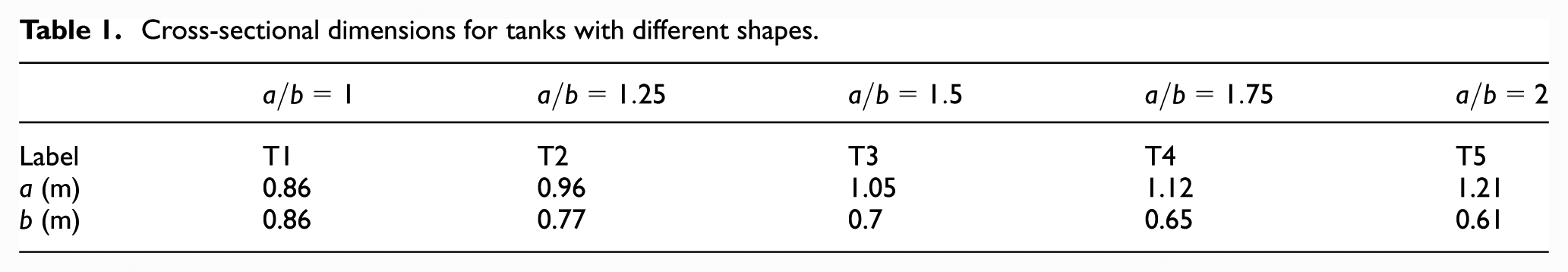
In Table 1, a and b are half of tank long and short axes, respectively. The ratio of long and short axis of elliptical tank cross sections changes from 1.0 to 2.0 with a step size of 0.25. The purpose of this setting is for a comprehensive commanding of liquid sloshing dynamics in tanks with different shapes. Furthermore, tanks with different cross sections in Table 1 were labeled as T1 to T5, and tank vehicles equipped with tanks in Table 1 were labeled as T1- to T5-vehicle for description convenience.

Rollover analysis of tank vehicles based on the estimation of liquid sloshing

The estimation of liquid sloshing

Liquid bulk is continuous medium, and sloshing force acting on tank wall in sloshing process is hard to obtain. To calculate sloshing force quickly and easily, the continuous liquid bulk is simplified to a mass point. The point has the same mass with liquid bulk, and its position coincides with the center mass of liquid bulk. Based on this assumption, sloshing force and torque on mass point can be expressed as

F_{y} = mg a_{y}; F_{z} = mg; M = \vec{r} \times \vec{F}

(1)

where F_y is lateral sloshing force, F_z is vertical sloshing force, M is sloshing torque on pivot or axis, $\vec{r}$ is the position vector, and $\vec{F}$ is force vector.

By equation (1), an estimation of liquid sloshing effects could be obtained. As liquid sloshing expressed by equation (1) is not related to time, flow distribution, liquid free surface, and so on, the method to evaluate liquid sloshing in partially filled tanks is quite convenient.

To analysis the influence of liquid sloshing on tanker’s driving stability, the position of mass point is also need to obtain. While the position of mass point coincides with the center of mass of liquid bulk, solution for the center of mass of liquid bulk will be carried out.

As shown in Figure 1, liquid free surface approximates to a tilted plane while lateral acceleration acting on tanks is quite small. Hence, a tilted straight line was used to describe the cross section of liquid free surface, as shown in Figure 1. While lateral acceleration acts on tank, the tank will rotate on the rollover axis and liquid free surface will tilt along the tank rotation direction. It was quite clear that the tilt angle of liquid free surface is related to lateral acceleration.

Figure 1.

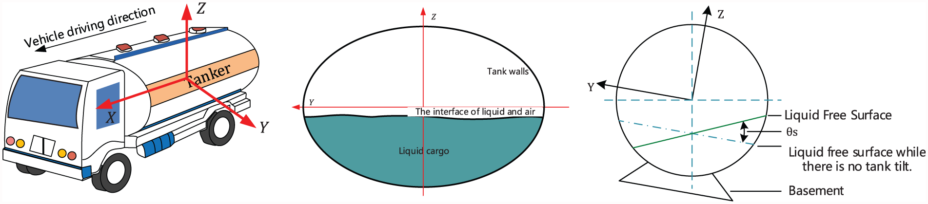
Tank-fixed coordinate.

By hydrostatic equilibrium equation, it can be given that

F_{X} dx + F_{Y} dy + F_{Z} dz = 0

(2)

where $F_{X}$ , $F_{Y}$ , and $F_{Z}$ are body forces of liquid bulk along X-axis, Y-axis, and Z-axis in tank-fixed coordinate (Figure 1), respectively.

Longitudinal liquid sloshing was not considered in this article, so there is no body force along X-axis. According to force analysis of liquid bulk along Y- and Z-axis, the tilt angle of liquid free surface can be expressed as

\tan θ_{s} = \frac{(a_{y} + ϕ)}{(1 - a_{y} ϕ)}

(3)

where θ_s is the tilt angle of liquid free surface, as shown in Figure 5; a_y is lateral acceleration acting on tanks; and $ϕ$ is tank’s roll angle.

Equation (3) indicates that the tilt angle of liquid free surface is not related to tank shape or fill level, but tank vehicle’s lateral acceleration and roll angle.

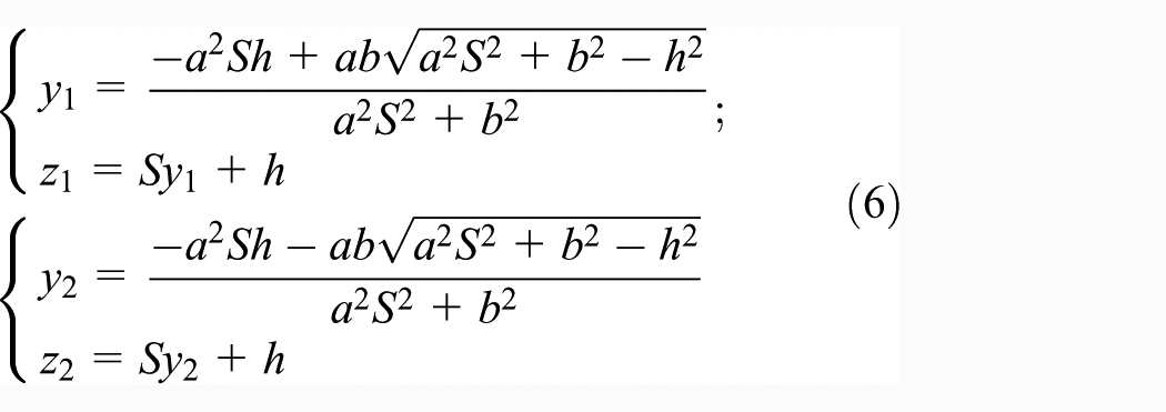
The intersection of liquid free surface and Z-axis was defined as h₀ when there is no lateral acceleration acting on tanks. With the action of lateral acceleration, level liquid free surface tilts and the intersection point changes, as shown in Figure 2. Under this condition, the cross section of liquid free surface can be presented as

z = Sy + h; S = \tan θ_{s}

(4)

where h is the intersection point of tilted liquid free surface and Z-axis.

Figure 2.

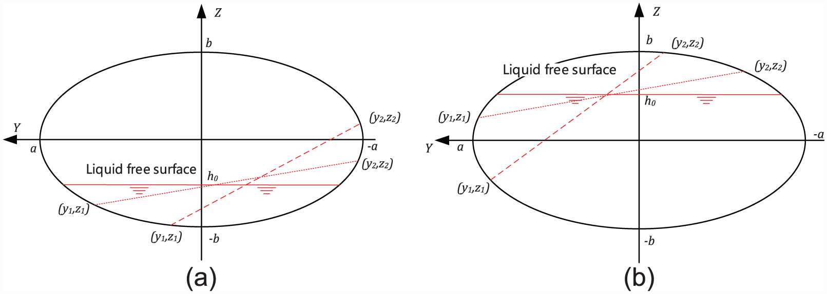
The intersection of liquid free surface and tank wall under different fill percentages: (a) liquid fill percentage less than or equal to 0.5 and (b) liquid fill percentage above 0.5.

For tanks with circular or elliptical cross sections, tank periphery can be expressed as

\frac{y^{2}}{a^{2}} + \frac{z^{2}}{b^{2}} = 1

(5)

Combined with equations (4) and (5), the intersection points of liquid free surface and tank walls are written as

\begin{array}{l} {\begin{matrix} y_{1} = \frac{- a^{2} S h + a b \sqrt{a^{2} S^{2} + b^{2} - h^{2}}}{a^{2} S^{2} + b^{2}} \\ z_{1} = S y_{1} + h \end{matrix}; \\ {\begin{matrix} y_{2} = \frac{- a^{2} S h - a b \sqrt{a^{2} S^{2} + b^{2} - h^{2}}}{a^{2} S^{2} + b^{2}} \\ z_{2} = S y_{2} + h \end{matrix} \end{array}

(6)

Cross-sectional area of liquid bulk when liquid free surface is tilted can be derived by equations (5) and (6). It was proved that the cross-sectional area of liquid bulk is a function of intersection point. However, no matter how liquid free surface tilts, the volume of liquid bulk and its cross-sectional area keep unchanged. While the cross-sectional area of liquid free surface can be obtained when tank dimensions and liquid fill percentage were given, the intersection point, h, can be obtained.

While the tilt angle of liquid free surface and the intersection point are already known, the center of mass of liquid bulk can be expressed as

Y_{1} = \frac{\int \int_{σ} ydydz}{\int \int_{σ} dydz}; Z_{1} = \frac{\int \int_{σ} zdydz}{\int \int_{σ} dydz}

(7)

By equation (7), moving trajectory of the center of mass of liquid bulk in sloshing process in tank with circular cross section is plotted in Figure 3. It was discovered that the moving trajectory of the center of mass of liquid bulk parallels to tank wall and its position can be written as

Y_{1} = (a - h_{cg 0} \frac{a}{b}) \sin θ_{s}; Z_{1} = b - (b - h_{cg 0}) \cos θ_{s}

(8)

where $h_{cg 0}$ is the center of mass of liquid bulk when liquid free surface is level.

Figure 3.

Moving trajectory of the center of mass of liquid bulk in circular tank.

Quasi-static modeling of tank vehicles

While sloshing forces and torques, and the postion of mass point are already known, rollover stability analysis of tank vehicles can be conducted. A typical tractor tank-semitrailer is plotted in Figure 4. The tank was separated into four chambers. The first and fourth chambers have the same volume, and the second and third chambers have the same volume. Besides, the volume of the first chamber is twice as much as the second one. For analysis convenience, the center of mass of tank-semitrailer’s sprung mass when vehicle is not laden was assumed to locate in the center of tank bracket.

Figure 4.

The distribution of Sprung mass.

Load distribution of vehicle’s three axes is presented as

{\begin{matrix} W_{s 1} = W_{f} + W_{fr} \\ W_{s 2} = W_{r} + W_{5} - W_{fr} \\ W_{s 3} = W_{t} + \sum W_{Li} - W_{5} \end{matrix}; {\begin{matrix} W_{1} = W_{s 1} + W_{u 1} \\ W_{2} = W_{s 2} + W_{u 2} \\ W_{3} = W_{s 3} + W_{u 3} \end{matrix}

(9)

where W_s₁, W_s₂, W_s₃ are sprung mass on 1-, 2-, and 3-axis, respectively; W_u₁, W_u₂, W_u₃ are un-sprung mass on 1-, 2-, and 3-axis, respectively; W₁, W₂, W₃ are qualities on 1-, 2-, and 3-axis, respectively; W_L is liquid quality; W_f, W_r are sprung mass on tractor’s front and rear axis when tractor does not haul a trailer; W₅ is the part of tank-trailer’s sprung mass that acts on saddle; W_fr is the part of W₅ that acts on 1-axis; W_t is the sprung mass of tank-semitrailer when the vehicle is not loaded.

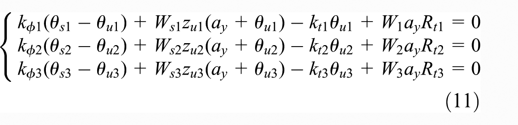
Roll moment equilibrium equations for sprung mass can be established according to Figure 5. The pivot of roll moment was the center of mass of sprung mass. For tank-semitrailer, the pivot of roll moment was the center of trailer bracket. Based on these assumptions, moment equilibrium equations for sprung mass are presented as

{\begin{matrix} - k_{ϕ 1} (θ_{s 1} - θ_{u 1}) + W_{s 1} z_{r 1} (a_{y} + θ_{u 1}) + k_{tr} (θ_{s 2} - θ_{s 1}) + W_{fr} z_{fr} (a_{y} + θ_{s 1}) = 0 \\ - k_{ϕ 2} (θ_{s 2} - θ_{u 2}) + W_{s 2} z_{r 2} (a_{y} + θ_{u 2}) - k_{tr} (θ_{s 2} - θ_{s 1}) - W_{fr} z_{fr} (a_{y} + θ_{s 2}) + W_{5} z_{52} (a_{y} + θ_{s 2}) + k_{c} (θ_{s 3} - θ_{s 2}) = 0 \\ - k_{ϕ 3} (θ_{s 3} - θ_{u 3}) + W_{s 3} z_{r 3} (a_{y} + θ_{u 3}) - W_{5} z_{53} (a_{y} + θ_{s 3}) - k_{c} (θ_{s 3} - θ_{s 2}) + \sum W_{Li} Z_{Li} (a_{y} + θ_{s 3}) + \sum W_{Li} Y_{Li} (1 - a_{y} θ_{s 3}) = 0 \end{matrix}

(10)

Figure 5.

Force analysis in vehicle’s roll plane.

Roll moment equilibrium equations for un-sprung mass are presented as

{\begin{matrix} k_{ϕ 1} (θ_{s 1} - θ_{u 1}) + W_{s 1} z_{u 1} (a_{y} + θ_{u 1}) - k_{t 1} θ_{u 1} + W_{1} a_{y} R_{t 1} = 0 \\ k_{ϕ 2} (θ_{s 2} - θ_{u 2}) + W_{s 2} z_{u 2} (a_{y} + θ_{u 2}) - k_{t 2} θ_{u 2} + W_{2} a_{y} R_{t 2} = 0 \\ k_{ϕ 3} (θ_{s 3} - θ_{u 3}) + W_{s 3} z_{u 3} (a_{y} + θ_{u 3}) - k_{t 3} θ_{u 3} + W_{3} a_{y} R_{t 3} = 0 \end{matrix}

(11)

where $k_{ϕ}$ is spring roll stiffness; $θ_{s}$ is roll angle of sprung mass; $θ_{u}$ is roll angle of un-sprung mass; z_r is the distance between the center of mass of sprung mass and roll axis; z_u is the distance between the center of mass of un-sprung mass and roll axis; z_fr is the distance from tractor bracket to roll axis; z₅ is the distance from saddle to roll axis; k_t is tire’s roll stiffness; R_t is tire’s rolling radius; k_c and k_tr are torsional stiffness of saddle and tractor bracket, respectively.

Parameter values for rollover analysis of tractor tank-semitrailer are listed in Table 2.

Table 2.

Parameter values for rollover analysis of tractor tank-semitrailer.

Parameters	Values	Parameters	Values	Parameters	Values
z_u ₁	0.131 m	z_u ₂	0.101 m	z_u ₃	0.1 m
z_fr	0.05 m	z ₅₂	−0.25 m	z ₅₃	0.35 m
z_r ₁	0.431 m	z_r ₂	0.331 m	z_r ₃	0.3 m
R_t ₁	0.55 m	R_t ₂	0.50 m	R_t ₃	0.45 m
k_tr	100,000 N m/rad	k_c	5,000,000 N m/rad	Tank length	12 m
k_t ₁	2,737,000 N m/rad	k_t ₂	2,660,000 N m/rad	k_t ₃	1,773,000 N m/rad
k_ϕ ₁	240,000 N m/rad	k_ϕ ₂	302,000 N m/rad	k_ϕ ₃	500,000 N m/rad

Define $x = [θ_{s 1}, θ_{s 2}, θ_{s 3}, θ_{u 1}, θ_{u 2}, θ_{u 3}]$ and $U = [0, 0, - W_{L} Y_{L}, 0, 0, 0]$ , then equations (10) and (11) can be rewritten as

Q x^{T} = P a_{y} - U^{T}

(12)

Quasi-static analysis on rollover threshold of tank vehicles

Numerical solution was done for equation (12). Liquid fill percentage changes from 0 to 1 with a step size of 0.1. Water was selected as the liquid cargo, whose density is 1000 kg/m³. Lateral acceleration acting on tractor tank-semitrailer when one side of wheel of 2- and 3-axis is just going to leave ground was used to describe tankers’ rollover threshold.

Simulation results are plotted in Figure 6. Rollover threshold for ordinary truck loaded with the same quality is also calculated.

Figure 6.

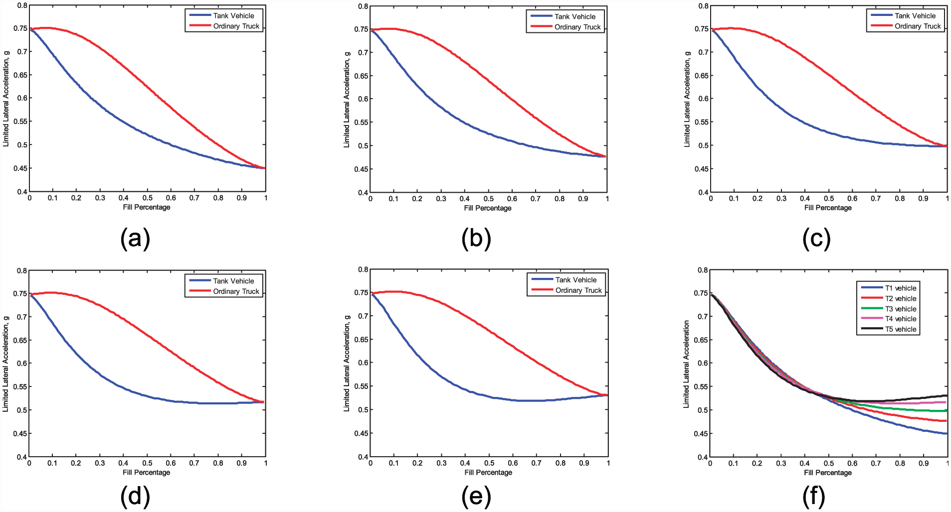
Rollover threshold for T1- to T5-vehicle by quasi-static method: (a) T1-vehicle, (b) T2-vehicle, (c) T3-vehicle, (d) T4-vehicle, (e) T5-vehicle, and (f) all vehicles’ rollover threshold.

Obviously, tank vehicles’ rollover stability decreases a lot compared with ordinary trucks, and the descending ratio reaches the biggest while liquid fill level is around 0.4. Therefore, the laden condition of 40% and its nearby fill level should be avoided in liquid transportation. However, while the estimation of vehicles’ rollover threshold is quasi-static, calculation results will be better than practical situations.

Figure 6 gives a comprehensive understanding of tank vehicles’ rollover threshold that equipped with tanks of different shapes. In the 5 kinds of tank vehicles, T1-vehicle has the best roll performance when liquid fill percentage is less than 0.5 but the worst roll stability when liquid fill level is above 0.5. T5-vehicle has the worst roll stability when liquid fill level is less than 0.5 but the best roll performance when liquid fill level is above 0.5. While in the most conditions fill percentage of tanks is above 0.5 for transportation economy, tanks with elliptical cross sections will be a better choice.

Rollover threshold of tank vehicles based on improved estimation of liquid sloshing

The comparison of practical liquid sloshing and its estimation result

Liquid free surface was simplified to a tilt plane when lateral acceleration is quite small. Under this assumption, the center of mass of liquid bulk was calculated, so does the position of mass point. However, with the increasement of external excitation, liquid sloshing amplitude grows and its free surface curves. To obtain the center of mass of liquid bulk, finite difference method was used. The cross section of liquid bulk was split into numbers of cells with sufficiently little area, and the center of mass of liquid bulk can be calculated by the center of each cell, which is presented as

y (t) = \frac{\sum_{c}^{liquid} y_{c} A_{c}}{\sum_{c}^{liquid} A_{c}}; z (t) = \frac{\sum_{c}^{liquid} z_{c} A_{c}}{\sum_{c}^{liquid} A_{c}}

(13)

where y(t) and z(t) are coordinates of the center of mass of liquid bulk, y_c and z_c are coordinates of liquid cell’s center, and A_c is liquid cell’s area.

Sloshing forces can be acquired according to the dynamic pressure that liquid cells acting on tank walls, which are written as

F_{y} (t) = \sum_{c}^{wet area} P_{c} B_{c} \cdot \vec{i}; F_{z} (t) = \sum_{c}^{wet area} P_{c} B_{c} \cdot \vec{j}

(14)

where F_y(t) and F_z(t) are lateral and vertical sloshing force, respectively; P_c is the pressure that liquid cell acts on tank wall; and B_c is the area of liquid cell that contacts with tank wall.

Sloshing torques on pointed pivot or axis can be expressed as

{\vec{M}}_{cg} (t) = \sum {\vec{r}}_{cg} (t) \times \vec{F} (t)

(15)

where r_cg(t) is position vector from the origin of the coordinate system to the point where the force is applied, and F(t) is force vector.

FLUENT simulation was done to obtain sloshing forces and the center of mass of liquid bulk. In simulation, liquid fill level changes from 0.4 to 0.8, and lateral acceleration acting on tank changes from 0.1g to 0.4g. The maximum, the minimum, and average values of sloshing forces in lateral and vertical directions, and the displacement of liquid bulk’s center of mass were calculated. The obtained results were compared with those obtained by estimation method, which are plotted in Figure 7.

Figure 7.

The practice liquid sloshing and its corresponding estimation results: (a) lateral sloshing force, (b) vertical sloshing force, (c) lateral displacement of center of mass, and (d) vertical displacement of center of mass.

Figure 7 shows that the average of each practical sloshing item are quite close to those obtained by the estimation method, respectively. To investigate the relation of practical sloshing effects and the estimated sloshing effects comprehensively, some ratios were calculated by

{\begin{matrix} F_{Y}_ratio = Mean (F_{Y}) / ES (F_{Y}) \\ F_{Z}_ratio = Mean (F_{Z}) / ES (F_{Z}) \\ C M_{Y}_ratio = Mean (C M_{Y}) / ES (C M_{Y}) \\ C M_{Z}_ratio = Mean (C M_{Z}) / ES (C M_{Z}) \end{matrix}

(16)

where CM denotes the displacement of liquid bulk’s center of mass and ES denotes estimation.

Ratio values when liquid fill level changes from 0.4 to 0.8 and lateral acceleration changes from 0.1g to 0.4g were calculated. The results showed that ratio values locate in the range of 0.991–0.999. This phenomenon proves that sloshing effects acquired by estimation method is the average of practical liquid sloshing. Therefore, rollover stability of tank vehicles obtained by quasi-static analysis will be conservative.

While the average of each practical liquid sloshing item can be obtained by estimation method conveniently, once the relation between the maximum of each practical liquid sloshing item and the estimated corresponding item is given, the maximum of sloshing forces, torques, and the displacement of center of mass of liquid bulk will be obtained easily. Therefore, the ratio of the maximum of each practical sloshing item to that obtained by estimation method is defined as

{\begin{matrix} F_{H} = \frac{Max (F_{Y})}{ES (F_{Y})} \\ F_{V} = \frac{Max (F_{z})}{ES (F_{z})} \\ C_{H} = \frac{Max (C M_{Y})}{ES (C M_{Y})} \\ C_{V} = \frac{Max (C M_{z})}{ES (C M_{z})} \end{matrix}

(17)

Where F_H, F_V, C_H, C_V are amplification coefficients of practical sloshing effects to estimated effects.

For tanks with circular cross section, amplification coefficients for sloshing forces and the displacement of center of mass are plotted in Figure 8. It was quite clear that amplification coefficients are functions of liquid fill percentage and lateral acceleration.

Figure 8.

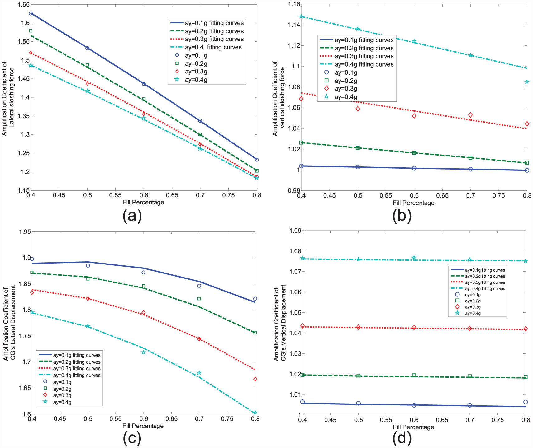
Amplification coefficients for liquid sloshing in tanks with circular cross section: (a) lateral sloshing force, (b) vertical sloshing force, (c) lateral displacement of center of mass, and (d) vertical displacement of center of mass.

The job of curves fitting was carried out to find the relation between amplification coefficients and liquid fill percentage and lateral acceleration. For T1, amplification coefficients can be expressed as

{\begin{matrix} C_{H} = 1.703 + 0.764 Δ + 0.402 a_{y} \\ - 0.711 Δ^{2} - 0.988 Δ a_{y} - 0.645 a_{y}^{2} \\ C_{V} = 0.984 + 0.032 Δ + 0.123 a_{y} \\ - 0.011 Δ^{2} - 0.15 Δ a_{y} - 0.518 a_{y}^{2} \\ F_{H} = 2.064 - 0.845 Δ - 1.073 a_{y} \\ - 0.176 Δ^{2} + 0.741 Δ a_{y} + 0.618 a_{y}^{2} \\ F_{V} = 0.997 + 0.0257 Δ - 0.010 a_{y} \\ + 0.001 Δ^{2} - 0.379 Δ a_{y} + 1.283 a_{y}^{2} \end{matrix}

(18)

where $Δ$ is liquid fill percentage.

For T2, amplification coefficients can be described as

{\begin{matrix} C_{H} = 2.392 + 1.034 Δ + 0.453 a_{y} - 0.973 Δ^{2} - 1.302 Δ a_{y} - 1.304 a_{y}^{2} \\ C_{V} = 0.881 + 0.023 Δ + 0.113 a_{y} - 0.005 Δ^{2} - 0.131 Δ a_{y} + 0.215 a_{y}^{2} \\ F_{H} = 2.057 - 0.493 Δ - 1.018 a_{y} - 0.507 Δ^{2} + 0.477 Δ a_{y} + 0.613 a_{y}^{2} \\ F_{V} = 0.787 + 0.534 Δ + 0.758 a_{y} - 0.295 Δ^{2} - 1.325 Δ a_{y} + 0.970 a_{y}^{2} \end{matrix}

(19)

For T3, amplification coefficients can be described as

{\begin{matrix} C_{H} = 3.18 + 1.311 Δ + 0.274 a_{y} - 1.25 Δ^{2} - 1.599 Δ a_{y} - 1.965 a_{y}^{2} \\ C_{V} = 0.810 + 0.017 Δ + 0.05 a_{y} - 0.004 Δ^{2} - 0.115 Δ a_{y} + 0.086 a_{y}^{2} \\ F_{H} = 2.047 - 0.232 Δ - 0.968 a_{y} - 0.732 Δ^{2} + 0.260 Δ a_{y} + 0.520 a_{y}^{2} \\ F_{V} = 0.904 + 0.002 Δ + 1.237 a_{y} + 0.147 Δ^{2} - 1.404 Δ a_{y} - 0.003 a_{y}^{2} \end{matrix}

(20)

For T4, amplification coefficients can be described as

{\begin{matrix} C_{H} = 4.056 + 1.587 Δ - 0.146 a_{y} - 1.534 Δ^{2} - 1.866 Δ a_{y} - 2.66 a_{y}^{2} \\ C_{V} = 0.754 + 0.01 Δ + 0.005 a_{y} - 0.1 Δ a_{y} - 0.047 a_{y}^{2} \\ F_{H} = 2.067 - 0.025 Δ - 1.443 a_{y} - 0.918 Δ^{2} + 0.321 Δ a_{y} + 1.358 a_{y}^{2} \\ F_{V} = 0.943 - 0.052 Δ + 1.052 a_{y} + 0.107 Δ^{2} - 0.864 Δ a_{y} - 0.392 a_{y}^{2} \end{matrix}

(21)

For T5, amplification coefficients can be described as

{\begin{matrix} C_{H} = 5.022 + 1.848 Δ - 0.878 a_{y} - 1.807 Δ^{2} - 2.128 Δ a_{y} - 3.213 a_{y}^{2} \\ C_{V} = 0.709 + 0.019 Δ - 0.093 a_{y} - 0.006 Δ^{2} - 0.089 Δ a_{y} - 0.050 a_{y}^{2} \\ F_{H} = 2.355 - 0.625 Δ - 2.33 a_{y} - 0.518 Δ^{2} + 0.790 Δ a_{y} + 2.574 a_{y}^{2} \\ F_{V} = 0.908 + 0.078 Δ + 1.005 a_{y} - 0.032 Δ^{2} - 0.530 Δ a_{y} - 0.804 a_{y}^{2} \end{matrix}

(22)

Combination with amplification coefficients, the maximum values of liquid sloshing effects can be acquired quite easily.

Rollover threshold of tank vehicles by improved quasi-static method

Rollover threshold of tractor tank-semitrailer was re-calculated by quasi-static method taking amplification coefficients into account. It was named as improved quasi-static method. Also, liquid fill percentage changes from 0 to 1 with a 0.1 step size, and water was the liquid cargo. Numerical solution results are presented in Figure 9. For comparison convenience, rollover threshold for ordinary truck with the same laden condition, as well as rollover threshold obtained by quasi-static method, is also plotted in Figure 9.

Figure 9.

Rollover threshold for T1- to T5-vehicle by improved quasi-static method: (a) T1-vehicle, (b) T2-vehicle, (c) T3-vehicle, (d) T4-vehicle, (e) T5-vehicle, and (f) rollover threshold of all vehicles.

It was found out that practical liquid sloshing has a quite significant effect on tank vehicles’ rollover stability. While amplification coefficients were took into consideration, tanker’s rollover threshold drops quite a lot compared to that of ordinary truck with the same laden condition. Calculation results showed that tank vehicles’ rollover threshold obtained by the improved quasi-static model descends about 20% compared with that obtained by quasi-static model. Fill level of 0.4 and its nearby values are laden conditions which should be avoided in practical transportation.

Figure 9 shows obviously that T5-vehicle has a much better roll performance when liquid fill percentage is above 0.45, and T1-vehicle has the worst roll performance at the same time. The roll stability of T2- to T4-vehicle locates in the middle position. Hence, tank with elliptical cross sections will be a better choice, especially those with longer long axis and shorter short axis.

Rollover analysis of tank vehicles based on equivalent mechanical model of liquid sloshing

Dynamic analysis of liquid sloshing in partially filled tanks

For tank vehicles, lateral liquid sloshing in partially filled tanks can be aroused by the changing of vehicle driving state. As a result, sloshing force acts on tank walls and decreases vehicle driving stability. Hence, before tankers’ dynamic modeling, dynamic analysis of liquid sloshing in partially filled tanks will be commenced first.

FLUENT was used to simulate liquid sloshing in partially filled tanks. Sloshing force, torque, and the center of mass of liquid bulk were recorded in the simulation. Lateral liquid sloshing can only be aroused in partially filled tank when lateral acceleration acting on it. For driving safety, tank vehicles’ lateral acceleration will not beyond 0.4g. There hence, lateral acceleration acting on tank will be smaller than or equal to 0.4g. Furthermore, longitudinal liquid sloshing was not considered in this article, and lateral liquid sloshing in different cross sections along tank’s longitudinal axis was assumed to be utterly the same with each other. So the three-dimensional liquid sloshing in tanks could be simplified to two-dimensional sloshing.

Simulation results for water sloshing while fill percentage is 40% are presented in Figure 10. Lateral acceleration acting on tank changes from 0.1g to 0.4g with a step size of 0.1g. It was quite obvious that external excitation has great effect on liquid sloshing. With the increase of lateral acceleration, shapes for liquid free surface change from linear to nonlinear. Liquid free surface could be described by a tilted plane when lateral acceleration is quite small (below 0.1g), and the curvature of liquid free surface is quite high when lateral acceleration is higher than 0.4g. Under this situation, the assumption of tilted plane on liquid free surface is no longer suitable.

Figure 10.

Liquid free surface in partially filled tanks under different lateral accelerations: (a) 0.1g, (b) 0.2g, (c) 0.3g, and (d) 0.4g.

Lateral sloshing forces monitored during the simulation are plotted in Figure 11. Quite obviously, sloshing force presents periodical characteristics. Furthermore, sloshing force corresponded with liquid free surface greatly. While lateral acceleration is small, curves for sloshing force can be approximately described by sine curves. In this situation, liquid sloshing could be defined as liner motion. Conclusions draw from liquid free surface and sloshing force are quite the same. With the increase of lateral acceleration, curve for sloshing force turns into irregular, and the liner motion of liquid sloshing turns into nonlinear one.

Figure 11.

Lateral sloshing force under different lateral accelerations: (a) 0.1g, (b) 0.2g, (c) 0.3g, and (d) 0.4g.

Inspired by the changing of liquid free surface and lateral sloshing force, it was assumed that liquid sloshing with small amplitude presents linear characteristic and its nonlinear feature grows gradually with sloshing amplitudes. To investigate sloshing dynamics more clearly, modal analysis for liquid sloshing in tanks with circular and elliptical cross section was conducted. The top six modal shapes are presented in Figures 12 and 13. It was found that the modal shapes of odd modals are anti-symmetrical and those of even modals are symmetrical. Therefore, it could be concluded that the odd modals contribute to the displacement of the center of mass of liquid bulk but the even ones do not. While the displacement of the center of mass of liquid bulk is the reason why lateral sloshing force generates, the anti-symmetrical modals produce sloshing force but the symmetrical modals do not. Besides, the first modal contributes the most to the displacement of the center of mass of liquid bulk and sloshing force, higher modals contribute quite little. Therefore, the first sloshing modal is the most important one.

Figure 12.

The top six modal shapes for liquid sloshing in partially filled tank with circular cross section: (a) the first modal, (b) the second modal, (c) the third modal, (d) the fourth modal, (e) the fifth modal, and (f) the sixth modal.

Figure 13.

The top six modal shapes for liquid sloshing in partially filled tank with elliptical cross section: (a) the first modal, (b) the second modal, (c) the third modal, (d) the fourth modal, (e) the fifth modal, and (f) the sixth modal.

More details about the dynamics of liquid sloshing in partially filled tanks without or with baffles can be found in Zheng et al.^37–39

Equivalent mechanical model for liquid sloshing

Dynamic analysis of liquid sloshing in partially filled tanks showed that liquid sloshing approximates to linear oscillation when external excitation is quite small. Besides, the modal analysis of liquid sloshing reveals that the first modal is the most important one to reflect the dynamics of liquid sloshing. Therefore, the first sloshing modal was chosen as the basement to establish equivalent mechanical model.

Trajectories of the center of mass of liquid bulk in liquid sloshing when external excitation changes from 0.1g to 0.4g were investigated and a part of results are plotted in Figure 14. The dashed line expresses ascending stage of the center of mass and the solid line describes descending stage. Numerical solution results showed that trajectory of the center of mass of liquid bulk in ascending stage approximately coincides with that in descending stage. This indicates that sloshing energy in a period does not lose much and its sloshing amplitude can be regarded as constant.

Figure 14.

Trajectories of the center of mass of liquid bulk in sloshing in tank with circular cross section: (a) external excitation is 0.1g and (b) external excitation is 0.4g.

Trajectories of the center of mass of liquid bulk were also proved to be approximately parallel to tank wall. Hence, a mechanical model that has the same motion trajectory with liquid bulk’s center of mass during sloshing can be used to describe liquid sloshing in tanks with elliptical cross sections. Thereafter, a trammel pendulum was selected to simulate liquid sloshing in tanks with elliptical cross sections, as plotted in Figure 15.

Figure 15.

Schematic diagram for the motion of trammel pendulum.

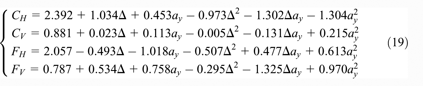
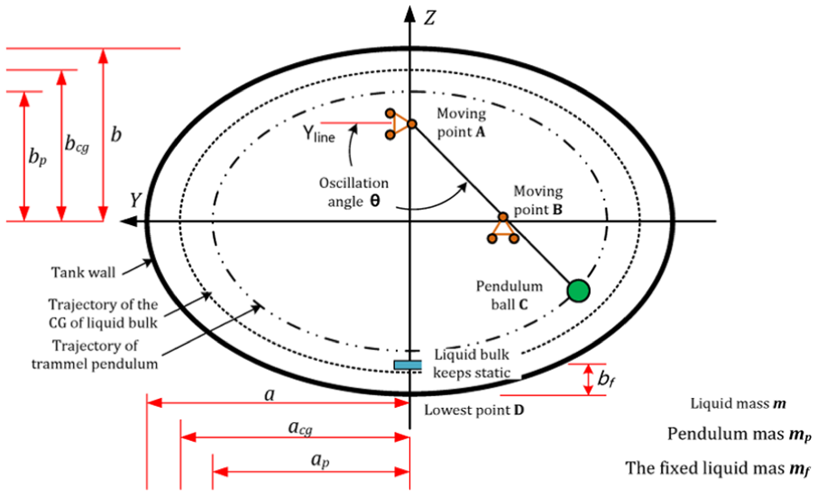
Sloshing trajectory and basic parameters of trammel pendulum are shown in Figure 15. Suppose that the pendulum’s moving trajectory is parallel to that of the center of mass of liquid bulk. The major axis of pendulum’s moving trajectory is equal to 2a_p and its minor axis is equal to 2b_p. Quite obviously, the ratio of a_p to b_p is equal to that of tank cross section’s major axis to its minor axis, which can be expressed as

\frac{a}{b} = \frac{a_{cg}}{b_{cg}} = \frac{a_{p}}{b_{p}} = ζ

(23)

Trammel pendulum’s arm length, which is the distance from moving point A to moving point B, is equal to a_p. A small ball with a certain quality, whose size is small enough to ignore, was attached to the free end of trammel pendulum’s arm. The distance from moving point B to pendulum ball is equal to b_p. Oscillation amplitude of trammel pendulum was defined as $θ$ , which is the angle from Y-axis to the arm of trammel pendulum.

As long as the original amplitude of trammel pendulum is not 90°, the pendulum will oscillate forth and back under the action of gravity. In tank-fixed coordinate, trammel pendulum’s oscillatory motion is plotted in Figures 16 and 17. Y_WZ_W are ground coordinate, whose Y_W- and Z_W-axis parallel to Y- and Z-axis, respectively. The Y_W-axis is tangent to tank’s lowest point and the Z_W-axis is tangent to tank’s leftmost point.

Figure 16.

Analytical diagram for the motion of trammel pendulum under inertial coordinate system.

Figure 17.

Analytical diagram for the motion of trammel pendulum under non-inertial coordinate system.

By Lagrange’s equations, the free oscillation of trammel pendulum can be expressed as

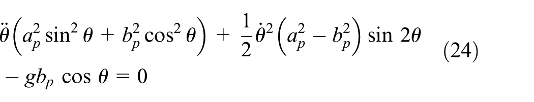
\begin{array}{l} \overset{\cdot\cdot}{θ} (a_{p}^{2} \sin^{2} θ + b_{p}^{2} \cos^{2} θ) + \frac{1}{2} {\dot{θ}}^{2} (a_{p}^{2} - b_{p}^{2}) \sin 2 θ \\ - g b_{p} \cos θ = 0 \end{array}

(24)

When tank moves laterally with constant velocity, the free oscillation of trammel pendulum still can be expressed by equation (24). Forced oscillation of trammel pendulum under inertial coordinate system can also be derived by Lagrange’s equations, which is written as

\begin{array}{l} \overset{\cdot\cdot}{θ} (a_{p}^{2} \sin^{2} θ + b_{p}^{2} \cos^{2} θ) + \frac{1}{2} {\dot{θ}}^{2} (a_{p}^{2} - b_{p}^{2}) \sin 2 θ \\ - g b_{p} \cos θ - \overset{\cdot\cdot}{y} a_{p} \sin θ = 0 \end{array}

(25)

In vehicle driving process, tank will rotate on roll axis while lateral acceleration acts on vehicle. Therefore, trammel pendulum will oscillate in non-inertia coordinate system. In this situation, the oscillatory motion of trammel pendulum is differential equations about its amplitude and tank’s roll angle, which is expressed as

{\begin{matrix} \overset{\cdot\cdot}{θ} (a_{p}^{2} \sin^{2} θ + b_{p}^{2} \cos^{2} θ) + \overset{\cdot\cdot}{ϕ} (a_{p} b_{p} - a_{p} b \sin θ) + \frac{1}{2} {\overset{\cdot}{θ}}^{2} (a_{p}^{2} - b_{p}^{2}) \sin 2 θ + {\overset{\cdot}{ϕ}}^{2} [\frac{1}{2} (a_{p}^{2} - b_{p}^{2}) \sin 2 θ + b_{p} b \cos θ] \\ - \overset{\cdot\cdot}{y} (a_{p} \sin θ \cos ϕ + b_{p} \cos θ \sin ϕ) + g (a_{p} \sin θ \sin ϕ - b_{p} \cos θ \cos ϕ) = 0 \\ \overset{\cdot\cdot}{ϕ} [{(b - b_{p} \sin θ)}^{2} + a_{p}^{2} \cos^{2} θ] + \overset{\cdot\cdot}{θ} (a_{p} b_{p} - a_{p} b \sin θ) + \overset{\cdot}{θ} \overset{\cdot}{ϕ} [\sin 2 θ (b_{p}^{2} - a_{p}^{2}) - 2 b_{p} b \cos θ] - {\overset{\cdot}{θ}}^{2} a_{p} b \cos θ \\ + \overset{\cdot\cdot}{y} (b \cos ϕ - a_{p} \cos θ \sin ϕ - b_{p} \sin θ \cos ϕ) + g [(b_{p} \sin θ - b) \sin ϕ - a_{p} \cos θ \cos ϕ] = 0 \end{matrix}

(26)

where $ϕ$ is tank’s roll angle.

Trammel pendulum’s dynamics was investigated according to equation (24). Its oscillatory motion with small and large amplitudes is presented in Figures 18 –20. Simulation results showed that oscillation amplitude effects the motion of trammel pendulum greatly. Small oscillation amplitude usually generates linear oscillation motion. With the increasement of oscillation amplitude, nonlinear characteristics keep growing and it can no longer be ignored. While the dynamics of trammel pendulum is quite similar with that of liquid sloshing, the usage of trammel pendulum to simulate liquid sloshing is suitable.

Figure 18.

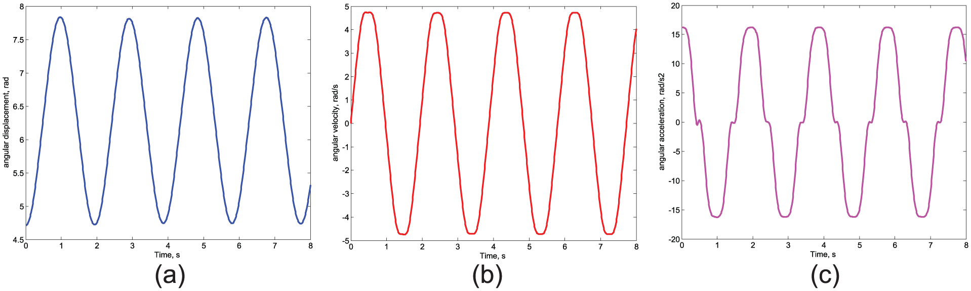
The motion of trammel pendulum when oscillation angle is 30°: (a) angular displacement, (b) angular velocity, and (c) angular acceleration.

Figure 19.

The motion of trammel pendulum when oscillation angle is 90°: (a) angular displacement, (b) angular velocity, and (c) angular acceleration.

Figure 20.

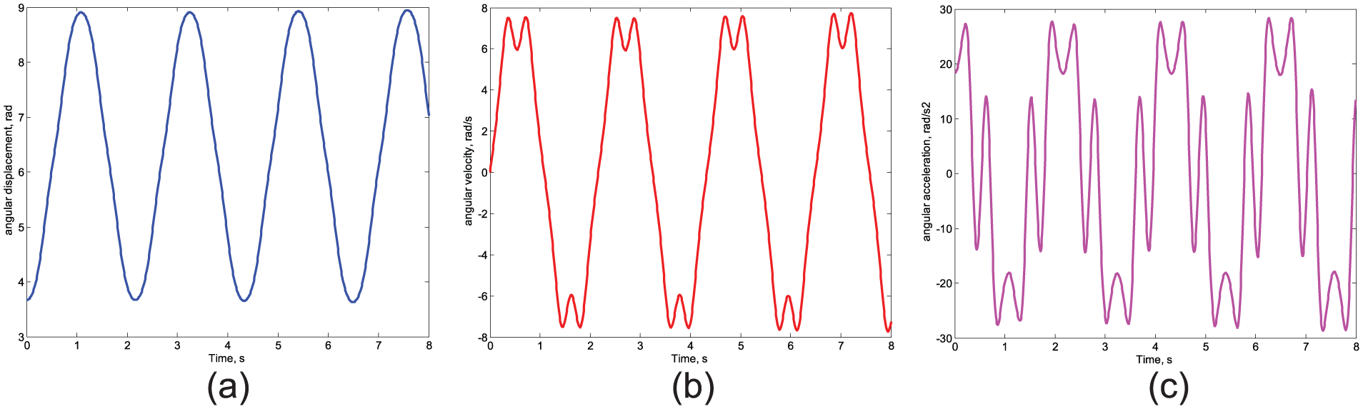
The motion of trammel pendulum when oscillation angle is 150°: (a) angular displacement, (b) angular velocity, and (3) angular acceleration.

Parameter values for trammel pendulum that should be given are presented in Figure 15. Due to the fact that not all of liquid cargo participates in sloshing, mass of pendulum ball is not equal to liquid quality. Thereafter, arm length a_p, pendulum mass m_p, fixed liquid mass m_f, and its position are parameters that should be calculated.

While trammel pendulum has dynamic characteristics just the same as liquid sloshing, by dynamics identity principle, the oscillation frequency of trammel pendulum is equal to liquid sloshing frequency. Besides, it was known that the oscillation frequency of trammel pendulum depends on its arm length. For a given tank loaded with specific volume of liquid cargo, sloshing frequency can be obtained by simulation. Therefore, the relation between arm length of pendulum and sloshing frequency should be investigated.

When oscillation amplitude of trammel pendulum is quite small, equation (24) can be rewritten as

\overset{\cdot\cdot}{θ} + (\frac{b_{p}^{2} - a_{p}^{2}}{a_{p}^{2}}) {\overset{\cdot}{θ}}^{2} θ + \frac{g b_{p}}{a_{p}^{2}} θ = 0

(27)

By analytical derivation, the phase plane trajectory equation of trammel pendulum is written as

\frac{d θ}{d t} = \sqrt{\frac{g b_{p}}{a_{p}^{2}}} \sqrt{θ_{\max}^{2} - θ^{2}}

(28)

At the instance of tanks with circular cross section, the coefficient of equation (28) is equal to $\sqrt{g / a_{p}}$ , which is the frequency expression for simple pendulums. Therefore, the phase plane trajectory equation of trammel pendulum is thus given by

\frac{d θ}{dt} = ω \sqrt{θ_{max}^{2} - θ^{2}}

(29)

Comparing equation (28) and (29), the natural oscillation frequency of trammel pendulum with small amplitude can be expressed as

ω = \sqrt{\frac{g b_{p}}{a_{p}^{2}}}

(30)

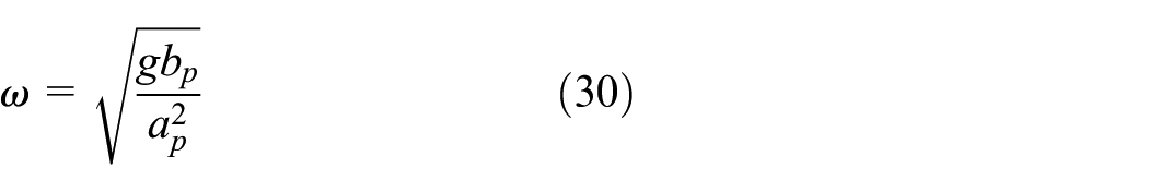
As the liquid sloshing frequency in a partially filled tank vehicle is already known, a_p and b_p can easily be obtained based on equations (23) and (30). When a pendulum is used to simulate liquid sloshing, the liquid mass that participates in sloshing is equal to the pendulum mass. According to the law of conservation of mass, the liquid mass that does not participate in sloshing is equal to the fixed part.

A direct solution for the pendulum mass is difficult and requires hydrodynamic theory analysis. Thus, an alternative method is used. First of all, suppose that all of the liquid mass participates in sloshing. If the maximum lateral acceleration of liquid bulk is known, then sloshing force generated by the entire liquid mass can be obtained. By comparing it with the actual sloshing force, the ratio of pendulum mass to the entire liquid mass can be acquired. Since the entire liquid mass is known, pendulum mass can thus be calculated.

According to Newton’s second law, sloshing force can be expressed by

F_{t} = m a_{ymax}

(31)

where F_t is sloshing force caused by the entire liquid mass, a_ymax is the maximum lateral acceleration of liquid bulk, and m is the entire liquid mass.

Lateral acceleration acting on tank vehicle is set to be zero, and liquid bulk oscillates only under the action of gravity. According to equation (24), the maximum lateral acceleration of liquid can be expressed as

a_{ymax} = max [a_{p} (- \overset{\cdot}{θ} \sin θ + \overset{\cdot\cdot}{θ} \cos θ)]

(32)

The actual maximum sloshing force is given by

F_{p} = max [m_{p} a_{y}]

(33)

Then liquid mass that participates in sloshing can be expressed as

\frac{m_{p}}{m} = \frac{F_{p}}{F_{t}}

(34)

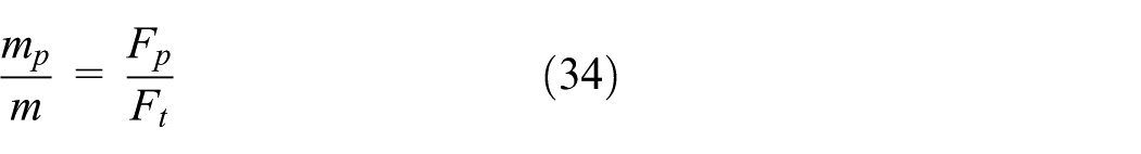
Thereafter, the fixed liquid mass can be expressed as

m_{f} = m - m_{p}

(35)

No matter where the locations of m_f and m_s are, the action point of the two parts always coincides with that of the center of mass of liquid bulk. Therefore, the center of mass of the fixed mass and the pendulum mass at the static location should coincide with the center of mass of liquid bulk, which can be expressed by

m_{f} (b - b_{f}) + m_{p} (b - b_{p}) = m (b - b_{cg})

(36)

While all the other parameters are already known, b_f can be obtained from equation (36). Until now, parametric expressions for trammel pendulum can be expressed as

{\begin{matrix} b_{p} = \frac{bg}{(ω^{2} ζ^{2} b)} \\ a_{p} = ζ b_{p} \\ m_{p} = \frac{m F_{p}}{F_{t}} \\ m_{f} = m - m_{p} \\ b_{f} = \frac{[m (b - b_{cg}) - m_{p} (b - b_{p})]}{m_{f}} \end{matrix}

(37)

Mass of liquid cargo in partially filled tank can be obtained by

m = ρ Vol

(38)

where ρ is liquid density and Vol is liquid volume.

Sloshing frequency and the maximum lateral sloshing force in T1–T5 tank were obtained by FLUENT simulation, as shown in Figures 21 and 22. For each tank, liquid fill percentage changes from 0.4 to 0.9 with a step size of 0.1. By equation (37), b_p and m_p can be obtained, as shown in Figures 23 and 24.

Figure 21.

Natural sloshing frequencies.

Figure 22.

Maximum sloshing forces.

Figure 23.

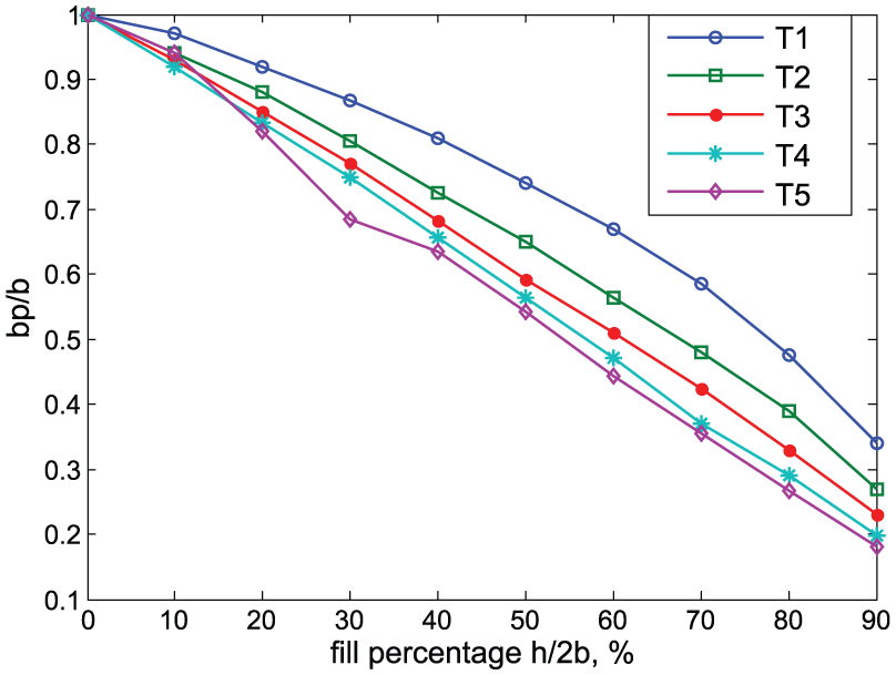
Values of b_p/b.

Figure 24.

Values of m_p/m.

Based on simulation results, curves fitting was done to discover the relationship between pendulum parameters and sloshing conditions. As a result, b_p and m_p can be presented as

{\begin{matrix} \frac{b_{p}}{b} = 1.087 + 0.6999 Δ - 0.1407 ζ - 0.9291 Δ^{2} - 1.178 ζ Δ + 0.05495 ζ^{2} - 0.03353 Δ^{3} + 0.5404 ζ Δ^{2} + 0.1518 ζ^{2} Δ \\ \frac{m_{p}}{m} = 0.7844 - 1.729 Δ + 0.3351 ζ + 1.156 Δ^{2} + 0.7256 ζ Δ - 0.1254 ζ^{2} - 0.3219 Δ^{3} - 0.9152 ζ Δ^{2} + 0.08043 ζ^{2} Δ \end{matrix}

(39)

To confirm the effectiveness of parameter values obtained above, forced liquid sloshing in T3 tank with a 0.6 liquid fill level was simulated. Lateral acceleration acting on tank is defined by

a_{y} = 0.2 \times 9.81 \times \sin (0.4 t)

(40)

Sloshing forces obtained by simulation are plotted in Figure 25. At the same time, they were also calculated by trammel pendulum model and plotted in Figure 25.

Figure 25.

Liquid sloshing forces under time-variant lateral excitation: (a) lateral sloshing force and (b) vertical sloshing force.

Comparison results showed that sloshing forces obtained by trammel pendulum coincide well with those acquired by computer simulation. Sloshing torque on special pivot was investigated to examine trammel pendulum carefully. The lowest point of tank, as shown in Figure 15, was chosen as the pivot. Forced liquid sloshing in T3 with different fill percentages was simulated. Lateral accelerations acting on tank chose 0.176g and 0.4g. Sloshing torques were collected during simulation, and they were also calculated by trammel pendulum model under the same condition. Simulation and calculation results are plotted in Figures 26 and 27.

Figure 26.

Sloshing torques on tank’s lowest point when lateral excitation is 0.176g: (a) fill level is equal to 0.1, (b) fill level is equal to 0.3, (c) fill level is equal to 0.6, and (d) fill level is equal to 0.9.

Figure 27.

Sloshing torques on tank’s lowest point when lateral excitation is 0.4g: (a) fill level is equal to 0.1, (b) fill level is equal to 0.3, (c) fill level is equal to 0.6, and (d) fill level is equal to 0.9.

When liquid fill level and lateral acceleration are both small, torque on tank’s lowest point obtained by calculation coincides well with that obtained by simulation both in frequency and in amplitude. Under this condition, the linear trammel pendulum can express liquid sloshing exactly. With the increase of liquid fill percentage, the nonlinear characteristics of liquid sloshing grow even under small external excitation. Then, the difference between practical liquid sloshing and trammel pendulum becomes bigger.

It can be seen from Figures 26 and 27 that external excitation has a great effect on the dynamics of liquid sloshing. When lateral acceleration is 0.4g and liquid fill level is 0.1, torque acquired by trammel pendulum can coincide well with that obtained by practical sloshing in frequency, and their magnitudes are quite close to each other. While liquid fill level increases to 0.3, torques obtained by the two methods differ in frequency and magnitude. The practical sloshing frequency is a little smaller than oscillation frequency of trammel pendulum, and practical torque amplitude is smaller than that obtained by pendulum. The difference both in frequency and in amplitude keep growing while liquid fill level increases. When liquid fill level is equal to 0.9, periodic feature for practical sloshing almost disappears, but trammel pendulum still oscillates periodically. Thereafter, the equivalent mechanical model should be used to express linear liquid sloshing or nonlinear sloshing whose nonlinear characteristics is not quite strong.

The dynamic modeling of tank vehicles

Dynamic modeling of tank vehicles based on equivalent mechanical model was conducted to investigate tanker’s roll stability exactly. To simplify the analysis of tank truck’s roll stability, some assumptions were made as follows:

Sprung mass is equal to vehicle mass that lies over the suspension system, in which liquid cargo is not included. In this article, vehicle and liquid bulk, as the solid and fluid parts, respectively, are not mixed with each other.

In the transverse direction, the center of mass of sprung mass locates at the bottom of the tank. Moreover, sprung mass is symmetrical about vehicle’s longitudinal axis.

Liquid sloshing is merely aroused along the transverse direction; sloshing in longitudinal direction is not taken into consideration. The movement and mass distribution of liquid bulk are completely the same at different tank cross sections along longitudinal direction, which means that the center of mass of liquid bulk located in the middle of the tank along the longitudinal direction.

Liquid free surface is not broken in driving.

Vehicle’s un-sprung mass is assumed not to produce roll movement.

Based on the above assumptions, a reference coordinate system for tanker dynamic analysis was established first. The origin of the coordinate is the point where the vertical line that goes through vehicle’s center of mass intersects with its roll axis (Figure 28). The back and top views of tanker’s dynamic analysis are plotted in Figures 29 and 30.

Figure 28.

The coordinate fixed on tank vehicles.

Figure 29.

The rollover analysis of tank vehicles.

Figure 30.

The lateral and yaw analysis of tank vehicles.

On the basis of Newton’s first law, when vehicle drives steadily, its inertial and external lateral forces reach a balance, which can be expressed as

m_{t} a_{s} + m_{f} a_{f} + m_{p} a_{pend} + m_{u} a_{u} = 2 (F_{f} + F_{r})

(41)

where a_s is lateral acceleration of sprung mass, a_u is lateral acceleration of un-sprung mass, a_f is lateral acceleration acting on fixed liquid mass, a_pend is lateral acceleration of pendulum ball, m_t is sprung mass, m_u is un-sprung mass, and F_f, F_r are the cornering force of front and rear tire, respectively.

In equation (41), lateral acceleration of sprung, un-sprung mass, and the fixed liquid mass are presented as

{\begin{matrix} a_{s} = V (\overset{\cdot}{β} + r) - h_{s} \overset{\cdot\cdot}{ϕ} + c \overset{\cdot}{r} \\ a_{u} = V (\overset{\cdot}{β} + r) - e \overset{\cdot}{r} \\ a_{f} = V (\overset{\cdot}{β} + r) - H_{1} \overset{\cdot\cdot}{ϕ} - e_{2} \overset{\cdot}{r} \end{matrix}

(42)

where V is vehicle driving speed, β is slip angle, r is yaw rate, h_s is the vertical distance between roll axis to the center of mass of sprung mass, c is the longitudinal distance from the center of mass of vehicle to that of sprung mass, and e is the longitudinal distance from the center of mass of vehicle to that of un-sprung mass.

Lateral acceleration acting on pendulum ball can be written as

a_{pend} = V (\overset{\cdot}{β} + r) + D_{1} \overset{\cdot\cdot}{ϕ} + D_{2} \overset{\cdot\cdot}{θ} + 2 D_{3} \overset{\cdot}{ϕ} \overset{\cdot}{θ} + D_{4} {\overset{\cdot}{ϕ}}^{2} + D_{5} {\overset{\cdot}{θ}}^{2}

(43)

where

{\begin{matrix} D_{1} = b \cos ϕ - a_{p} \cos θ \sin ϕ - b_{p} \sin θ \cos ϕ \\ D_{2} = - (a_{p} \sin θ \cos ϕ + b_{p} \cos θ \sin ϕ) \\ D_{3} = a_{p} \sin θ \sin ϕ - b_{p} \cos θ \cos ϕ \\ D_{4} = b_{p} \sin θ \sin ϕ - b \sin ϕ - a_{p} \cos θ \cos ϕ \\ D_{5} = - a_{p} \cos θ \cos ϕ + b_{p} \sin θ \sin ϕ \end{matrix}

(44)

According to moment balance between vehicle inertia and external moment, vehicle’s roll and yaw moment balance equation can be expressed as

{\begin{matrix} I_{z} \overset{\cdot}{r} - I_{xz} \overset{\cdot\cdot}{ϕ} - m_{p} a_{pend} e_{2} - I_{xzp} (\overset{\cdot\cdot}{ϕ} + {\overset{\cdot\cdot}{θ}}_{2}) + I_{zzp} \overset{\cdot}{r} \\ - I_{xyp} (\overset{\cdot}{ϕ} + {\overset{\cdot}{θ}}_{2})^{2} - I_{yzp} r (\overset{\cdot}{ϕ} + {\overset{\cdot}{θ}}_{2}) = 2 (F_{f} l_{f} - F_{r} l_{r}) \\ I_{x} \overset{\cdot\cdot}{ϕ} - I_{xz} \overset{\cdot}{r} - (m_{t} h_{s} + m_{f} H_{1}) V (\overset{\cdot}{β} + r) - m_{p} a_{pend} (h_{s} + b) \\ + I_{xxp} (\overset{\cdot\cdot}{ϕ} + {\overset{\cdot\cdot}{θ}}_{2}) - I_{xzp} \overset{\cdot}{r} + I_{xyp} r (\overset{\cdot}{ϕ} + {\overset{\cdot}{θ}}_{2}) + I_{yzp} r^{2} \\ = - k_{ϕ} ϕ - c_{ϕ} \overset{\cdot}{ϕ} + ϕ (m_{t} g h_{s} + m_{f} g H_{1} + m_{p} g (h_{s} + b)) + m_{p} g a_{pend} \cos θ \end{matrix}

(45)

where l_f is the distance between vehicle’s center of mass to front axis; l_r is the distance between vehicle’s center of mass to rear axis; $c_{ϕ}$ is sprung roll damping; e₂ is the longitudinal distance from liquid bulk’s center of mass to that of vehicle; H₁ is the vertical distance from fixed liquid mass to roll axis; I_x, I_z are vehicle’s moment of inertia on x-axis and z-axis, respectively; I_xz is vehicle’s inertia product on x- and z-axis; I_xxp, I_yyp, I_zzp are moment of inertia of pendulum ball on x-, y-, and z-axis, respectively; I_xyp, I_xzp, I_yzp are moment product of pendulum ball on x- and y-axis, x- and z-axis, y- and z-axis, respectively.

Tank vehicle’s dynamic characteristics can be expressed by equations (26), (41), and (45). Slip angle, yaw rate, roll angle of tank vehicle, as well as pendulum oscillation amplitude, are degree of freedoms to describe vehicle handling stability.

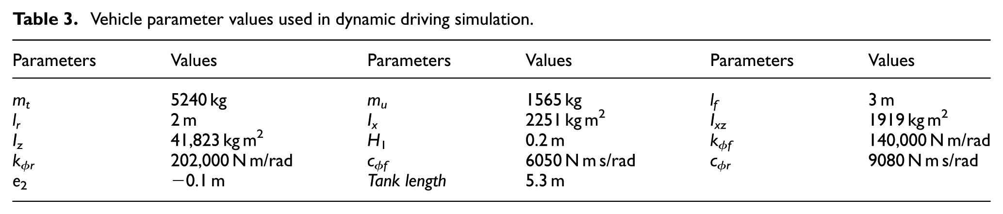
XH9140G, a typical tank semi-trailer of PieXin brand, is chosen as the research object in this part.²⁷ Vehicle parameter values used in simulation are listed in Table 3.

Table 3.

Vehicle parameter values used in dynamic driving simulation.

Parameters	Values	Parameters	Values	Parameters	Values
m_t	5240 kg	m_u	1565 kg	l_f	3 m
l_r	2 m	I_x	2251 kg m²	I_xz	1919 kg m²
I_z	41,823 kg m²	H ₁	0.2 m	k_ϕf	140,000 N m/rad
k_ϕr	202,000 N m/rad	c_ϕf	6050 N m s/rad	c_ϕr	9080 N m s/rad
e ₂	−0.1 m	Tank length	5.3 m

Dynamic analysis on tank vehicles’ roll stability

Steady-state circular test

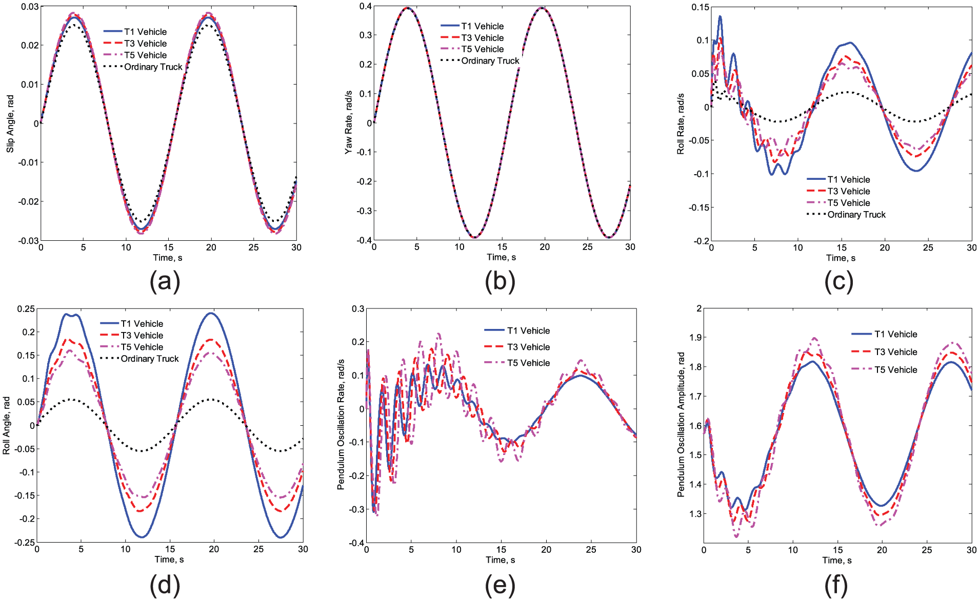
Tank vehicle’s dynamic response in steady-state circular test was carried out numerically to discover its dynamic roll stability. Vehicle driving speed was set to be 20 m/s, and steering wheel angle is 0.1 rad. Liquid fill level changes from 0.2 to 0.9 with a 0.1 step size. Water was chosen as liquid cargo. During numerical simulation, slip angle, yaw rate, roll angle, and roll rate were collected. Angular displacement and velocity of trammel pendulum were also recorded. Part of simulation results is plotted in Figure 31. T1-, T3-, and T5-vehicle were selected as representatives. For comparison convenience, dynamic response of ordinary truck is also presented in Figure 31.

Figure 31.

Dynamic response of tank vehicle with 80% laden state in steady-state circular test: (a) slip angle, (b) yaw rate, (c) roll rate, (d) roll angle, (e) pendulum oscillation rate, and (f) pendulum oscillation amplitude.

Damping feature is not considered in the establishment of equivalent mechanical model. Therefore, oscillation features obtained by tank vehicle’s dynamic models are stronger than practical situations.

It is obvious that tank vehicle’s roll stability is greatly influenced by transient liquid sloshing. While roll angle of ordinary truck quickly returns to steady state, that of tank truck fluctuates up and down for about 20 s before turning into steady, and the overshoot is quite large. However, the overshoot dampens quickly with the passage of time. When vehicle’s driving state turns into stable, roll angle for ordinary truck is about 0.05 rad. Under the same condition, roll angles for T1-, T3-, and T5-vehicle are about 0.25, 0.18, and 0.15 rad, respectively.

The influence of liquid sloshing on lateral stability is quite small due to the fact that yaw rates for ordinary and tank trucks are quite close to each other. Besides, the difference between slip angle for ordinary and tank trucks is also quite small.

With the passage of time, trammel pendulum’s oscillation amplitude drops greatly with the aid of lateral acceleration and gravity. Thereafter, sloshing forces and torques are apt to reach a constant value.

Serpentine test

Tank vehicle’s dynamic response in serpentine test was also conducted to discover tanker’s dynamic characteristics comprehensively. Vehicle driving speed was also set to be 20 m/s. A sinusoidal wheel angle input is given, which can be expressed as

δ = 0.1 \sin (0.4 t)

(46)

Cargo fill level changes from 0.2 to 0.9 with a 0.1 step size. Numerical solution results are plotted in Figure 32.

Figure 32.

Dynamic response of tank vehicle with 80% laden state in serpentine test: (a) slip angle, (b) yaw rate, (c) roll rate, (d) roll angle, (e) pendulum oscillation rate, and (f) pendulum oscillation amplitude.

In the situation of time-varying steering wheel angle input, vehicle dynamic response has the same frequency with that of steering wheel angle input. For tank vehicle, amplitudes of slip angle, roll rate, and roll angle are all bigger than those of ordinary trucks. Particularly, tank vehicle’s roll angle is much bigger than that of ordinary truck. Under the same condition, the maximum roll angle of ordinary truck, and T5-, T3-, and T1-vehicle are 0.05, 0.155, 0.18, and 0.24 rad, respectively.

In vehicle driving, the oscillation of trammel pendulum was decided by its natural feature and wheel angle input. Oscillation amplitude of lower frequency is much bigger than that of higher frequency; hence, the influence of inherent oscillation on tank vehicle’s dynamic response is significantly covered.

Analysis of tank vehicles’ roll stability

It was discovered that tank vehicle’s roll stability is greatly influenced by transient liquid sloshing, while tanker’s lateral stability is not impacted greatly by it. Besides, tank vehicles assembled with different tanks have quite different roll stabilities. To command roll stability of tank vehicles comprehensively, roll angles for T1- to T5-vehicle in a steady-state circular test were calculated. Liquid fill level for each tanker changes from 0.2 to 0.9. At the same time, roll angle for ordinary truck with the same laden condition was also calculated.

Rate of decline was chosed to be the indicator to express roll stability of tank vehicles. The indicator can be obtained by

rate of decline = \frac{(ϕ_{o} - ϕ_{t})}{ϕ_{o}}

(47)

where $ϕ_{o}$ is roll angle of ordinary truck; $ϕ_{t}$ is roll angle of tank truck.

Calculation results are plotted in Figure 33.

Figure 33.

Rate of decline for T1- to T5-vehicle.

Calculation results showed T1-vehicle has the worst roll stability and T5-vehicle has the best roll stability. It reveals that tank shape has a giant effect on tanker’s roll stability. Sloshing in tanks with flat cross sections do less influence on tanker’s roll stability. The possible reason for this phenomenon lies in the dimension that the displacement of liquid bulk’s center of mass along vertical direction in tanks with elliptical cross section is smaller than that in tanks with circular cross section. With the increase of the ratio of tank’s major axis to its minor axis, the displacement of liquid bulk’s center of mass along vertical direction drops and the impact of transient liquid sloshing on vehicle’s roll stability decrease. On the other hand, the displacement of liquid bulk’s center along lateral direction in tanks with elliptical cross section is larger than that in tanks with circular cross section. Combined with the roll stability performance of tank vehicles, it should be derived that the lateral displacement of liquid bulk’s center of mass in sloshing is of much less significance than the vertical displacement.

Liquid fill level also has a great influence on tank vehicle’s roll stability. When liquid fill level is quite small, decline rate of tank vehicle’s roll stability is below 0.2, no matter what shape the tank has. With liquid fill level increases, the decline rate grows quickly and it reaches the biggest value when liquid fill level is about 0.6. Liquid fill level still keeps increasing but the decline rate drops gradually. Therefore, tank vehicle’s roll stability is greatly influenced when the liquid fill level is nearby 0.6. In this situation, tank vehicle’s roll stability is much worse than that of ordinary trucks. However, when the liquid fill level is either fairly small or large, tank vehicle’s roll stability is only slightly influenced by sloshing. There hence, liquid fill level of 0.4–0.6 is the worst laden situation which should be avoided.

A much interesting discovery is that the T3-vehicle divides tank vehicles into two parts. For T1- and T2- vehicle, they have much worse roll stability than T3-vehicle. However, for T4- and T5-vehicle, they have quite similar roll stability to that of T3-vehicle. While large major axis makes tank has quite wide dimension, there is no need to lengthen major axis of tank cross section any more when its ratio of major axis to minor axis reaches to 1.5. Hence, elliptical tank whose major axis to minor axis is equal to 1.5 will be a good choice for tank vehicles.

Discussion

As a fluid-solid coupling system, tank vehicle’s dynamic modeling must take liquid sloshing into account. The conventional solution on liquid sloshing dynamics by hydrodynamics is difficult and time-consuming. Therefore, three different methods to describe liquid sloshing effects in partially filled tanks with elliptical cross sections are proposed in this article. Then, the work of tank vehicles’ dynamic modeling was commenced based on that.

The first method simplified continuous liquid bulk as a mass point and used the motion of this mass point to represent liquid sloshing. While dynamic features of liquid sloshing were somewhat neglected by this method, dynamic model of tank vehicle established on this simplification was named as quasi-static model. Rollover analysis by quasi-static model showed that tank vehicles’ rollover threshold decreases a lot compared with that of ordinary trucks. The quasi-static analysis on tankers’ roll stability is quite easy, but the result is of low accuracy. Under the situation of estimate tankers’ rollover threshold roughly, the quasi-static method can be used.

To improve the accuracy of sloshing estimation, the relationship between practical liquid sloshing and its estimation effect was investigated. Amplification coefficients were used to express the relation between the maximum of each practical sloshing item and its estimated result, and they were took into account in the quasi-static model. Rollover threshold obtained by improved quasi-static model showed that tankers’ roll stability is quite worse than ordinary trucks, and T5-vehicle has the best roll stability in the whole range of liquid fill level among five tankers. Results obtained by improved quasi-static method differ a little with those obtained by quasi-static method.

The estimation on liquid sloshing could not reflect its dynamic features. There hence, a trammel pendulum model was proposed and established to simulate liquid sloshing in partially filled tanks. The pendulum has the same dynamic characteristics with liquid sloshing. Based on that, dynamic modeling of tankers was conducted and rollover analysis was done. It was found out that tank vehicles’ dynamic response to steering angle input fluctuates up and down around the steady value. It will take a quite long time for vehicle comes into steady stage. It was also discovered that a liquid fill level of 0.4–0.6 is the worst laden situation and should be avoided. Roll stability analysis for tank vehicles on the basis of equivalent mechanical model could reflect vehicle’s dynamic characteristics, and the results are with much accuracy.

The trammel pendulum established in this article could simulate linear or weakly nonlinear liquid sloshing with great accuracy. However, for strongly nonlinear liquid sloshing, sloshing effect obtained by the trammel pendulum will have great error from actual conditions. Therefore, equivalent mechanical models for nonlinear liquid sloshing will be a study direction in the near future.

Footnotes

Academic Editor: Hai Xiang Lin

Declaration of conflicting interests

The author(s) declared no potential conflicts of interest with respect to the research, authorship, and/or publication of this article.

Funding

The author(s) disclosed receipt of the following financial support for the research, authorship, and/or publication of this article: The research is supported by the National Natural Science Foundation of China (grant no. 51375200) and the Opening Project of Key Laboratory of Operation Safety Technology on Transport Vehicles, Ministry of Transport, PRC.

References

Woodrooffe

. Evaluation of dangerous goods vehicle safety performance. Report TP 13678-E, Transport Canada, 2000.

Douglas

Kate

Nancy

. Cargo tank roll stability study: final report. Report GS23-0011L, 2007. Washington, DC: US Department of Transportation.

Kwon

. Conditional value-at-risk model for hazardous material transportation. In: Proceedings of the 2011 winter simulation conference (WSC), Phoenix, AZ, 11–14 December 2011, pp.1703–1709. New York: IEEE.

Treichel

Hughes

Barkan

CPL

. Safety performance of tank cars in accidents: probabilities of lading loss. Report RA-05e02, 2006. Washington, DC: RSI-AAR Railroad Tank Car Safety Research and Test Project, Association of American Railroads.

Wuhong

Katsushi

. Reliability and safety analysis methodology for identification of drivers’ erroneous actions. Int J Automot Techn 2010; 11: 873–881.

Wuhong

Wei

Hongwei

. A safety-based behavioural approaching model with various driving characteristics. Transport Res C: Emer 2011; 19: 1202–1214.

Solaas

Faltinsen

OM.

Combined numerical and analytical solution for sloshing in two-dimensional tanks of general shape. J Ship Res 1997; 41: 118–129.

Modaressi-Tehrani

Rakheja

Stiharu

Three-dimensional analysis of transient slosh within a partly-filled tank equipped with baffles. Vehicle Syst Dyn 2007; 45: 525–548.

Popov

Sankar

. Dynamics of liquid sloshing in horizontal cylindrical road containers. Proc IMechE, Part C: J Mechanical Engineering Science 1993; 207: 399–406.

10.

Akyildiz

A numerical study of the effects of the vertical baffle on liquid sloshing in two-dimensional rectangular tank. J Sound Vib 2012; 331: 41–52.

11.

Hasheminejad

Aghabeigi

Liquid sloshing in half-full horizontal elliptical tanks. J Sound Vib 2009; 324: 332–349.

12.

Rumold

Modeling and simulation of vehicle carrying liquid cargo. Multibody Syst Dyn 2001; 5: 351–374.

13.

Toumi

Bouazara

Richard

MJ.

Impact of liquid sloshing on the behavior of vehicles carrying liquid cargo. Eur J Mech A: Solid 2009; 28: 1026–1034.

14.

Guorong

Rakheja

Siddiqui

Experimental study of liquid slosh dynamics in a partially-filled tank. J Fluid Eng: T ASME 2009; 131: 071303.1–071303.14.

15.

Romero

Ramírez

Fortanell

. Analysis of lateral sloshing forces within road containers with high fill levels. Proc IMechE, Part D: J Automobile Engineering 2006; 220: 303–312.

16.

Modaressi-Tehrani

Rakheja

Sedaghati

Analysis of the overturning moment caused by transient liquid slosh inside a partly filled moving tank. Proc IMechE, Part D: J Automobile Engineering 2006; 220: 289–301.

17.

Chunyu

Jincheng

Studies on liquid sloshing in rigid containers using FLUENT code. J Shanghai Jiaotong Univers 2008; 42: 593–596.

18.

Strandberg

Lateral stability of road tankers. VIT report 138A, 1978. Linköping: National Road and Traffic Research Institute.

19.

Ranganathan

Rakheja

Steady turning stability of partially filled tank vehicles with arbitrary tank geometry. J Dyn Syst: T ASME 1989; 111: 481–495.

20.

Rangaanathan

Rollover threshold of partially filled tank vehicles with arbitrary tank geometry. Proc IMechE, Part D: J Automobile Engineering 1993; 207: 241–244.

21.

Sankar

Surial

A sensitivity analysis approach for fast estimation of rollover stability heavy articulated vehicles during steady state turning. Heavy Veh Syst 1994; 1: 282–303.

22.

Kang

Rakheja

Stiharu

. Optimal tank geometry to enhance static roll stability of partially filled tank vehicles. SAE technical paper 1999-01-3730, 1999.

23.

Kang

Rakheja

Stiharu

Cargo load shift and its influence on tank vehicle dynamics under braking and turning. Int J Heavy Veh Syst 2002; 9: 173–203.

24.

Winkle

. Rollover of heavy commercial vehicles. Umtri Research Review, Report-UMTRI-99019, 2001.

25.

Zheng

Liu

HF.

Improved algorithm on roll stability evaluation of partially filled tractor-tank semitrailer. J Jilin Univers 2012; 42: 1089–1094 (in Chinese).

26.

Dodge

. Chapter 6. Analytical representation of lateral sloshing by equivalent mechanical models. In: Abramson

Silverman

(eds) The dynamic behavior of liquids in moving containers (special publication NASA SP-106). Washington, DC: National Aeronautics and Space Administrator, 1966, pp.199–224.

27.

Abramson

Chu

Kana

DD.

Some studies of nonlinear lateral sloshing in rigid containers. J Appl Mech 1966; 33: 777.

28.

Salem

MI.

Rollover stability of partially filled heavy-duty elliptical tankers using trammel pendulums to simulate fluid sloshing. PhD Thesis, Department of Mechanical and Aerospace Engineering, West Virginia University, Morgantown, WV, 2000.

29.

Zheng

Ren

YY.

Equivalent mechanical model for lateral liquid sloshing in partially-filled tank vehicles. Math Probl Eng 2012; 2012: 162825 (22 pp.).

30.

Abramson

HN.

The dynamic behavior of liquids in moving containers. NASA SP-106, 1966. Washington, DC: NASA.

31.

Qing

Xingrui

Tianshu

Equivalent mechanical model for liquid sloshing during draining. Acta Astronaut 2011; 68: 91–100.

32.

Utsumi

A mechanical model for low-gravity sloshing in an axisymmetric tank. J Appl Mech: T ASME 2004; 71: 724–730.

33.

Love

Tait

MJ.

Equivalent linearized mechanical model for tuned liquid dampers of arbitrary tank shape. J Fluid Eng: T ASME 2011; 133: 061105 (9 pp.).

34.

Ranganathan

Ying

Miles

Analysis of fluid slosh in partially filled tanks and their impact on the directional response of tank vehicles. SAE Transactions 1993; 102: 502–505.

35.

Ranganathan

Rakheja

Sankar

Directional response of a B-train vehicle combination carrying liquid cargo. J Dyn Syst: T ASME 1993; 115: 133–139.

36.

Dai

Setiawan

A new non-linear approach to analysing the dynamic behaviour of tank vehicles subjected to liquid sloshing. Proc IMechE, Part K: J Multi-body Dynamics 2005; 219: 75–86.

37.

Zheng

Ren

. Modal analysis of transient liquid sloshing in partially-filled tanks. Appl Mech Mater 2014; 526: 127–132.

38.

Zheng

Ren

. Transient liquid sloshing in partially-filled tank vehicles. Appl Mech Mater 2014; 526: 133–138.

39.

Zheng

Ren

. Effects of transverse baffle design on reducing liquid sloshing in partially filled tank vehicles. Math Probl Eng 2013; 2013: 130570 (13 pp.).

Rollover stability analysis of tank vehicles based on the solution of liquid sloshing in partially filled tanks

Abstract

Keywords

Introduction

Tank shapes

Rollover analysis of tank vehicles based on the estimation of liquid sloshing

The estimation of liquid sloshing

Quasi-static modeling of tank vehicles

Quasi-static analysis on rollover threshold of tank vehicles

Rollover threshold of tank vehicles based on improved estimation of liquid sloshing

The comparison of practical liquid sloshing and its estimation result

Rollover threshold of tank vehicles by improved quasi-static method

Rollover analysis of tank vehicles based on equivalent mechanical model of liquid sloshing

Dynamic analysis of liquid sloshing in partially filled tanks

Equivalent mechanical model for liquid sloshing

The dynamic modeling of tank vehicles

Dynamic analysis on tank vehicles’ roll stability

Steady-state circular test

Serpentine test

Analysis of tank vehicles’ roll stability

Discussion

Footnotes

Declaration of conflicting interests

Funding

References