Sage Journals: Discover world-class research

Abstract

Liquid sloshing in the tank of a tank truck is one of the important factors affecting the driving stability of the tank truck. When the external motivation is larger, the liquid sloshing phenomenon shows the nonlinear characteristics of the movement, causing rollover accidents. Therefore, it is of practical significance to study the movement of a tank car to improve its stability. Based on the equivalent pendulum mechanical model under nonlinear condition, the liquid sloshing nonlinear motion of a tank was investigated. A simulated liquid sloshing test bench was used to verify the validity of the nonlinear model. This study provides a theoretical basis to improve the driving stability of a tank truck.

Keywords

Tank truck driving stability nonlinear liquid sloshing motion equivalent mechanical model dynamic response

Introduction

Because of the effect of liquid density and road axle weight restrictions, liquid sloshing in a partially filled tank is the main cause of the decrease in the driving stability of a tank truck. By simulating liquid sloshing, the liquid sloshing motion of a tank truck is evaluated. This type of motion is similar to reciprocating oscillation and associated with the reciprocating motion of a simple mechanical structure. If the back-and-forth movement of a mechanical structure is used to describe the liquid sloshing movement in a tank, the stability problem of a tank truck can be solved using a liquid sloshing dynamics model. For the best stability of a tank truck, an oval cross section is obtained using a simulation test bench test.

Because of many adverse factors of numerical simulation, an equivalent mechanical model, mechanical dynamics theory, was established and widely used. This method converts fluid dynamics into a mechanical movement to study liquid sloshing in a tank. In the 20th century (1950s and 1960s), scholars used a spring system and the pendulum model to simulate the liquid sloshing phenomenon,^1–4 but they mainly focused on rockets and spacecrafts. Graham established the equivalent pendulum model and used to describe the static vibration of a free surface when a liquid sloshed in a tank. In 1952, Graham and Rodrigues developed another model; it is based on the principle that a vibrating liquid is equivalent to a point mass (sloshing point mass). Both the ends are connected to a spring, and the spring is fixed at the other end of the tank wall. The residual liquid that does not participate in the vibration is considered as a fixed rigid mass. In 1964, Pinson⁵ deduced the spring constants of oval tanks filled with a liquid propellant. A linear numerical model of liquid sloshing in a tank can effectively describe this phenomenon. For nonlinear sloshing dynamics, attention should be paid to the model of inherent nonlinear unit. The nonlinear rotational freedom of a liquid surface can be understood by introducing the spherical pendulum model.^6–8 Georgia Institute of Technology,⁹ Bauer and Eidel,¹⁰ and Bauer et al.¹¹ studied the nonlinear mechanism to describe the free surface movement. In 1966, Abramson¹² studied the load with a circular cross section of lateral liquid sloshing in a tank and found that under lateral excitation, the vortex amplitude of a partially filled cylinder or spherical tank varies. Kana¹³ and Unruh et al.¹⁴ established a spherical pendulum model to simulate the nonlinear rotational impact; a part of the liquid motion can be simulated by the spherical pendulum model. The corresponding vibration throughout the first vibration and the residual liquid can be simulated by the basic linear pendulum model. Using the general fluid analysis software FLUENT, the volume of fluid (VOF) method was used to define the free surface, establish a turbulence model, determine liquid sloshing by calculation, and obtain the nonlinear dynamic response of liquid sloshing during the driving of a tank truck.¹⁵ In 1992, Sankar¹⁶ considered the nonlinear characteristics of a liquid in an oval cross-section tank stated previously in the literature to explore the tank liquid sloshing theory using the linear theory, but the study was limited to a small vibration field. Some of the parameters in common use and amplitude range were proposed; some nonlinear parts cannot be ignored. It was concluded that one of the most important parameters, the lateral acceleration for an approximate circular cross section, under more than 50% filled tank condition should not be more than 0.2g (m/s²).

In simulation experiments using a liquid sloshing simulation test bench, it was concluded that the tank liquid sloshing phenomenon has both linear and nonlinear motion features; therefore, it is important to establish a numerical simulation model to study the characteristics of the phenomenon.¹⁷ Based on the pendulum equivalent mechanical model, a liquid pendulum sloshing model under nonlinear excitation was developed.

Liquid pendulum sloshing model under nonlinear excitation

Using the equivalent mechanical model to describe liquid sloshing in a tank, the pendulum movement is determined by the liquid storage tank movement. According to the motion and structure of a tank truck, the movement of the tank can be divided into translation, rotation, and complex motion (combination of translational and rotational motion), exhibiting strong nonlinear characteristics.

During the movement of a tank truck, the tank will tilt to one side due to centrifugal force, as shown in Figure 1; the pendulum model involves translational and rotational motions.

Figure 1.

Pendulum model (a combination of translational and rotational motions).

As shown in Figure 1, the displacement $\vec{r}$ can be expressed as follows

\vec{r} = \vec{R} + \vec{d} + \vec{b}

(1)

\vec{R} = yi + zj

(2)

\vec{b} = b \sin φ i + b \cos φ j

(3)

\vec{d} = [(a_{p} \cos φ - b_{p} \sin φ \tan θ) \cos θ] i + [\begin{matrix} (a_{p} \cos φ - b_{p} \sin φ \tan θ) \sin θ + \\ b_{p} \sin φ / \cos θ \end{matrix}] j

(4)

\vec{r} = [\begin{matrix} (a_{p} \cos φ - b_{p} \sin φ \tan θ) \cos θ + \\ y + b \sin φ \end{matrix}] i + [\begin{matrix} (a_{p} \cos φ - b_{p} \sin φ \tan θ) \sin θ + \\ b_{p} \sin φ / \cos θ + b \cos φ + z \end{matrix}] j

(5)

\begin{matrix} \vec{\dot{r}} = {\begin{cases} [- \dot{φ} (a_{p} \sin φ + b_{p} \cos φ \tan θ) - \dot{θ} b_{c g} \sin φ (1 + \tan^{2} θ)] \cos θ - \\ \dot{θ} (a_{p} \cos φ - b_{p} \sin φ \tan θ) \sin θ + \dot{y} + \dot{φ} b \cos φ \end{cases}} i \\ + {\begin{cases} [- \dot{φ} (a_{p} \sin φ + b_{p} \cos φ \tan θ) - \dot{θ} b_{p} \sin φ (1 + \tan^{2} θ)] \sin θ + \\ \dot{θ} (a_{p} \cos φ - b_{p} \sin φ \tan θ) \cos θ + \dot{φ} b_{p} \cos φ / \cos θ + \\ \dot{θ} b_{p} \sin φ \sin θ / \cos^{2} θ + \dot{z} - \dot{φ} b \sin φ \end{cases}} j \end{matrix}

(6)

In formula (6)

\begin{matrix} ζ = \overset{\cdot}{φ} (b \cos φ + b_{p} \cos φ \sin θ - a_{p} \sin φ \cos θ) \\ - \overset{\cdot}{θ} (a_{p} \sin θ \cos φ + b_{p} \sin φ \cos θ) + \overset{\cdot}{y} \end{matrix}

(7)

\begin{matrix} ξ = \overset{\cdot}{φ} (b \sin φ - a_{p} \sin φ \sin θ - b_{p} \cos φ \cos θ) \\ + \overset{\cdot}{θ} (a_{p} \cos φ \cos θ - b_{p} \sin φ \sin θ) + \overset{\cdot}{z} \end{matrix}

(8)

Formula (6) can be rewritten as follows

\vec{\overset{\cdot}{r}} = ζ i + ξ j

(9)

\vec{\overset{\cdot\cdot}{r}} = \overset{\cdot}{ζ} i + \overset{\cdot}{ξ} j

(10)

{\vec{\overset{\cdot}{r}}}^{2} = ζ^{2} + ξ^{2}

(11)

According to the Lagrange function

L = T - V

(12)

The kinetic energy of the pendulum model can be expressed as follows

T = \frac{1}{2} m {\vec{\overset{\cdot}{r}}}^{2} = \frac{1}{2} m (ζ^{2} + ξ^{2})

(13)

The potential energy of the pendulum model can be expressed as follows

V = mg (\begin{matrix} b - (a_{p} \cos φ - b_{p} \sin φ \tan θ) \sin θ - \\ b_{p} \sin φ / \cos θ \end{matrix}) \cos θ

(14)

By substituting formulas (13) and (14) into formula (12), the Lagrange function of the pendulum can be obtained. Using the Lagrange motion equation, the partial derivative φ of the Lagrange function L can be expressed as follows

\frac{\partial L}{\partial φ} = \frac{1}{2} m (\frac{\partial (ζ^{2})}{\partial φ} + \frac{\partial (ξ^{2})}{\partial φ}) - \frac{\partial V}{\partial φ} = m (ζ \frac{\partial ζ}{\partial φ} + ξ \frac{\partial ξ}{\partial φ}) - \frac{\partial V}{\partial φ}

(15)

$\partial ζ / \partial φ$ , $\partial ξ / \partial φ$ , and $\partial V / \partial φ$ can be expressed as follows

\begin{matrix} \frac{\partial ζ}{\partial φ} = - {\overset{\cdot}{φ}}^{2} (b_{t} \sin φ + b_{p} \sin φ \sin θ - a_{p} \cos φ \cos θ) - \overset{\cdot}{φ} \overset{\cdot}{θ} (b_{p} \cos φ \cos θ - a_{p} \sin φ \sin θ) \end{matrix}

(16)

\begin{matrix} \frac{\partial ξ}{\partial φ} = {\overset{\cdot}{φ}}^{2} (b_{t} \cos φ + b_{p} \sin φ \sin θ - a_{p} \sin φ \cos θ) - \overset{\cdot}{φ} \overset{\cdot}{θ} (b_{p} \cos φ \sin θ + a_{p} \sin φ \cos θ) \end{matrix}

(17)

\frac{\partial V}{\partial φ} = g \overset{\cdot}{φ} \cos θ [(a_{p} \sin φ + b_{p} \sin φ \tan θ) \sin θ - b_{p} \frac{\cos φ}{\cos θ}]

(18)

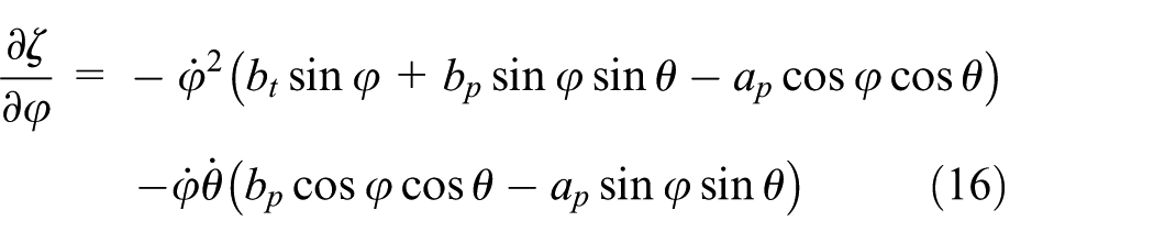
The partial derivative $\overset{\cdot}{φ}$ of the Lagrange function L can be expressed as follows

\frac{\partial L}{\partial \overset{\cdot}{φ}} = \frac{1}{2} m (\frac{\partial (ζ^{2})}{\partial \overset{\cdot}{φ}} + \frac{\partial (ξ^{2})}{\partial \overset{\cdot}{φ}}) - \frac{\partial V}{\partial \overset{\cdot}{φ}} = m (ζ \frac{\partial ζ}{\partial \overset{\cdot}{φ}} + ξ \frac{\partial ξ}{\partial \overset{\cdot}{φ}}) - \frac{\partial V}{\partial \overset{\cdot}{φ}}

(19)

$\partial ζ / \partial \overset{\cdot}{φ}$ , $\partial ξ / \partial \overset{\cdot}{φ}$ , and $\partial V / \partial \overset{\cdot}{φ}$ can be expressed as follows

\frac{\partial ζ}{\partial \overset{\cdot}{φ}} = b_{t} \cos φ + b_{p} \cos φ \sin θ - a_{p} \sin φ \cos θ

(20)

\frac{\partial ξ}{\partial \overset{\cdot}{φ}} = b_{t} \sin φ - a_{p} \sin φ \sin θ - b_{p} \cos φ \cos θ

(21)

\frac{\partial V}{\partial \overset{\cdot}{φ}} = 0

(22)

The partial derivative t of $\partial L / \partial \overset{\cdot}{φ}$ can be expressed as follows

\frac{\partial}{\partial t} (\frac{\partial L}{\partial \overset{\cdot}{φ}}) = \frac{1}{2} m ({\frac{\partial (ζ^{2})}{\partial \overset{\cdot}{φ}} |}_{t} + {\frac{\partial (ξ^{2})}{\partial \overset{\cdot}{φ}} |}_{t}) = m (\overset{\cdot}{ζ} \frac{\partial ζ}{\partial \overset{\cdot}{φ}} + {{ζ \overset{\cdot\cdot}{φ} \frac{\partial ζ}{\partial \overset{\cdot}{φ}} |}_{t} + \overset{\cdot}{ξ} \frac{\partial ξ}{\partial \overset{\cdot}{φ}} + ξ \overset{\cdot\cdot}{φ} \frac{\partial ξ}{\partial \overset{\cdot}{φ}} |}_{t})

(23)

In the Lagrange motion equation, the relationship between formulas (19) and (23) can be expressed as follows

\frac{1}{2} m ({\frac{\partial (ζ^{2})}{\partial \overset{\cdot}{φ}} |}_{t} + {\frac{\partial (ξ^{2})}{\partial \overset{\cdot}{φ}} |}_{t}) - {\frac{\partial V}{\partial \overset{\cdot}{φ}} |}_{t} - \frac{1}{2} m (\frac{\partial (ζ^{2})}{\partial φ} + \frac{\partial (ξ^{2})}{\partial φ}) - \frac{\partial V}{\partial φ} = 0

(24)

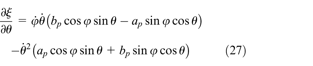
Using the Lagrange motion equation, the partial derivative θ of the Lagrange function L can be expressed as follows

\frac{\partial L}{\partial θ} = \frac{1}{2} m (\frac{\partial (ζ^{2})}{\partial θ} + \frac{\partial (ξ^{2})}{\partial θ}) - \frac{\partial V}{\partial θ} = m (ζ \frac{\partial ζ}{\partial θ} + ξ \frac{\partial ξ}{\partial θ}) - \frac{\partial V}{\partial θ}

(25)

$\partial ζ / \partial θ$ , $\partial ξ / \partial θ$ , and $\partial V / \partial θ$ can be expressed as follows

\frac{\partial ζ}{\partial θ} = \overset{\cdot}{φ} \overset{\cdot}{θ} (b_{p} \cos φ \cos θ + a_{p} \sin φ \sin θ) - {\overset{\cdot}{θ}}^{2} (a_{p} \cos φ \cos θ - b_{p} \sin φ \sin θ)

(26)

\frac{\partial ξ}{\partial θ} = \overset{\cdot}{φ} \overset{\cdot}{θ} (b_{p} \cos φ \sin θ - a_{p} \sin φ \cos θ) - {\overset{\cdot}{θ}}^{2} (a_{p} \cos φ \sin θ + b_{p} \sin φ \cos θ)

(27)

\frac{\partial V}{\partial θ} = m g \dot{θ} (\begin{array}{l} b_{p} \sin φ \sin θ (1 + \tan^{2} θ) - (a_{p} \cos φ - b_{p} \sin φ \tan θ) \cos θ - \\ \frac{b_{p} \sin φ \sin θ}{\cos^{2} θ} - (\begin{array}{l} b_{t} - (a_{p} \cos φ - b_{p} \sin φ \tan θ) \sin θ - \\ b_{p} \sin φ / \cos θ \end{array}) \sin θ \end{array})

(28)

\frac{\partial L}{\partial \overset{\cdot}{θ}} = \frac{1}{2} m (\frac{\partial (ζ^{2})}{\partial \overset{\cdot}{θ}} + \frac{\partial (ξ^{2})}{\partial \overset{\cdot}{θ}}) - \frac{\partial V}{\partial \overset{\cdot}{θ}} = m (ζ \frac{\partial ζ}{\partial \overset{\cdot}{θ}} + ξ \frac{\partial ξ}{\partial \overset{\cdot}{θ}}) - \frac{\partial V}{\partial \overset{\cdot}{θ}}

(29)

$\partial ζ / \partial \overset{\cdot}{θ}$ , $\partial ξ / \partial \overset{\cdot}{θ}$ , and $\partial V / \partial \overset{\cdot}{θ}$ can be expressed as follows

\frac{\partial ζ}{\partial \overset{\cdot}{θ}} = a_{p} \sin θ \cos φ + b_{p} \sin φ \cos θ

(30)

\frac{\partial ξ}{\partial \overset{\cdot}{θ}} = a_{p} \cos φ \cos θ - b_{p} \sin φ \sin θ

(31)

\frac{\partial V}{\partial \overset{\cdot}{θ}} = 0

(32)

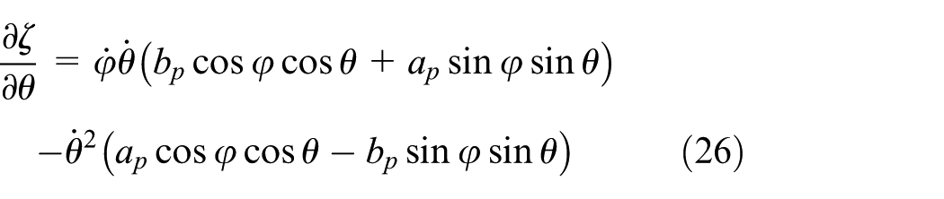
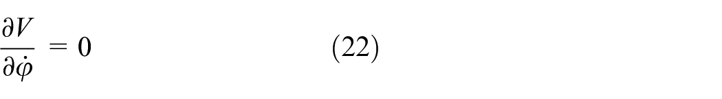
The partial derivative $\overset{\cdot}{θ}$ of L can be expressed as follows

\begin{matrix} \frac{\partial}{\partial t} (\frac{\partial L}{\partial \overset{\cdot}{θ}}) = \frac{1}{2} m ({\frac{\partial (ζ^{2})}{\partial \overset{\cdot}{θ}} |}_{t} + {\frac{\partial (ξ^{2})}{\partial \overset{\cdot}{θ}} |}_{t}) - {\frac{\partial V}{\partial \overset{\cdot}{θ}} |}_{t} \\ = m (\overset{\cdot}{ζ} \frac{\partial ζ}{\partial \overset{\cdot}{θ}} + {{ζ \overset{\cdot\cdot}{θ} \frac{\partial ζ}{\partial \overset{\cdot}{θ}} |}_{t} + \overset{\cdot}{ξ} \frac{\partial ξ}{\partial \overset{\cdot}{θ}} + ξ \overset{\cdot\cdot}{θ} \frac{\partial ξ}{\partial \overset{\cdot}{θ}} |}_{t}) \end{matrix}

(33)

${\frac{\partial ζ}{\partial \overset{\cdot}{θ}} |}_{t}$ and ${\frac{\partial ξ}{\partial \overset{\cdot}{θ}} |}_{t}$ can be expressed as follows

{\frac{\partial ζ}{\partial \overset{\cdot}{θ}} |}_{t} = \overset{\cdot}{θ} (a_{p} \cos θ \cos φ - b_{p} \sin φ \sin θ)

(34)

{\frac{\partial ξ}{\partial \overset{\cdot}{θ}} |}_{t} = - \overset{\cdot}{θ} (a_{p} \cos φ \sin θ + b_{p} \sin φ \cos θ)

(35)

In the Lagrange motion equation, the relationship between formulas (29) and (33) can be expressed as follows

\frac{1}{2} m ({\frac{\partial (ζ^{2})}{\partial \overset{\cdot}{θ}} |}_{t} + {\frac{\partial (ξ^{2})}{\partial \overset{\cdot}{θ}} |}_{t}) - {\frac{\partial V}{\partial \overset{\cdot}{θ}} |}_{t} - \frac{1}{2} m (\frac{\partial (ζ^{2})}{\partial θ} + \frac{\partial (ξ^{2})}{\partial θ}) - \frac{\partial V}{\partial θ} = 0

(36)

Formula (36) is the nonlinear differential equation of the movement of pendulum model under the translational and rotational excitation.

Parameters of nonlinear pendulum model

Determination of cycloid length of pendulum model

The liquid oscillation frequency is determined from the sloshing frequency (C), angular frequency (1/ω), length of free surface (p), and instantaneous maximum sloshing force under different liquid level conditions, as shown in Table 1.

Table 1.

Liquid sloshing frequency and the maximum sloshing force.

Cross section	Liquid level (%)	Sloshing frequency (Hz)	Sloshing angular frequency (rad/s)	Maximum sloshing force (N)
Oval	50	1.084	12.566	9.6
	60	1.146	10.471	10.2
	70	1.228	8.975	9.8
	80	1.349	7.853	8.7
	90	1.578	6.981	6.4

The sloshing angular frequency can be expressed as follows

{\begin{matrix} T = 1 / C \\ ω = 2 π / T \end{matrix}

(37)

When the oval cross-section size of tank a_t = 0.26, b_t = 0.175, the liquid vibration frequency and the maximum sloshing force in the oval tank are shown in Table 1. When the liquid level increases, the sloshing frequency also increases. Liquid sloshing frequency and angular frequency vary with the liquid level, as shown in Figures 2 and 3. When the liquid level increases, the liquid sloshing frequency also increases, but the liquid sloshing angular frequency decreases.

Figure 2.

Liquid sloshing frequency variation with the liquid level.

Figure 3.

Liquid sloshing angular frequency variation with the liquid level.

The relationship between b_p and b can be expressed as follows

b_{p} = \frac{g}{ω^{2} ς^{2}}

(38)

As shown in Figure 4, when the liquid level increases, the length of the cycloid decreases. In equation (38), V was determined using equation (14); b_p and b are included in equation (14); equation (14) is substituted into formula (38) and the relationships b_p and b are obtained. When the liquid level is higher, the liquid sloshing phenomenon is weaker.

Figure 4.

Cycloid length variation with the liquid level.

Determination of liquid sloshing quality on pendulum model

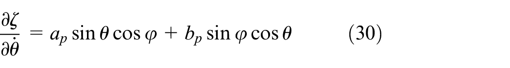
Figure 5 shows the instantaneous maximum sloshing force with the change in liquid level. When the liquid level is more than 60%, the instantaneous maximum sloshing force is the maximum. As the liquid level increases, the instantaneous maximum sloshing force decreases. In the nonlinear model of the pendulum, the relationship between pellet quality and the total mass of liquid can be expressed as follows

m = m_{f} + m_{p}

(39)

The relationship between pellet quality and the instantaneous maximum sloshing force can be expressed as follows

\frac{m_{p}}{m} = \frac{F_{p}}{F_{t}} = \frac{F_{p}}{max (m a_{y})}

(40)

where F_p is the instantaneous maximum sloshing force, N. m_p/m varies with the liquid ratio, as shown in Figure 6. When the liquid level increases, the pendulum ball quality is less proportional.

Figure 5.

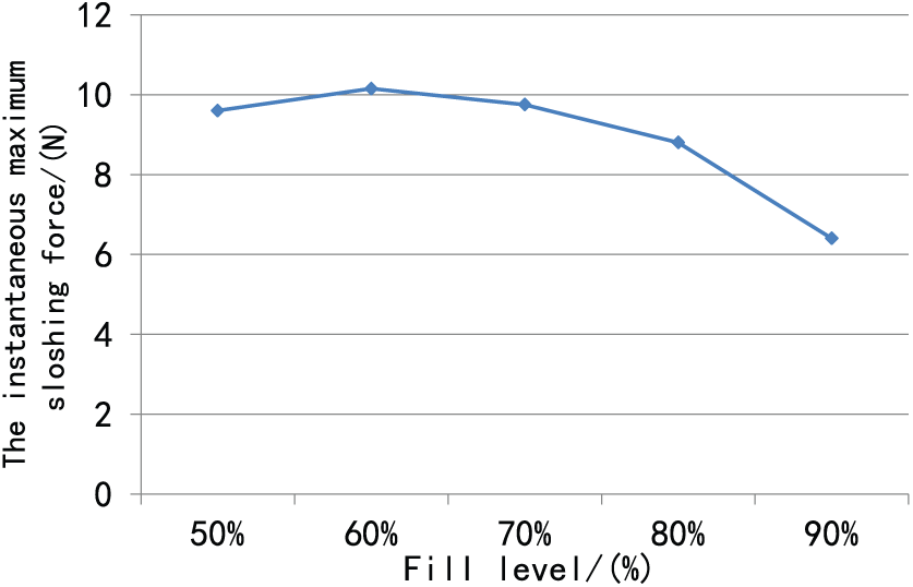
Instantaneous maximum sloshing force variation with liquid level.

Figure 6.

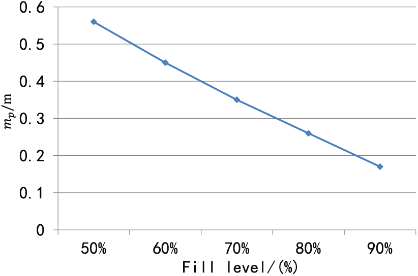
m_p/m variation with the liquid level.

Analysis of the nonlinear pendulum model of liquid sloshing

Numerical simulation analysis of the nonlinear pendulum model

The lateral force is the strength index of liquid sloshing phenomenon in oval tanks. As shown in Figure 7, the nonlinear dynamic model for lateral sloshing changes from 0.9 Hz to the external excitation. When the time was varied from 1 to 1.6 s, the lateral force increased; the lateral force decreased from 3 to 3.6 s. This trend is different from 1 to 1.6 s in lateral force. After 3.5 s, the lateral force showed a smooth trend; therefore, the liquid nonlinear motion did not increase infinitely because of the increase in the external motivation. Because of the damping of the liquid, the internal damping liquid balances the system’s dissipation of energy.

Figure 7.

Nonlinear model of simulation calculation for lateral sloshing force: (a) 1–1.6 s, (b) 3–3.6 s, and (c) 0–10 s.

Comparison and analysis of nonlinear pendulum model with ANSYS Fluent

A nonlinear pendulum model was established using the ANSYS Fluent fluid mechanics simulation software; the data of sloshing force were compared with the results of numerical simulation nonlinear model.

The ANSYS Fluent software used for the modeling of tank is shown in Figure 8. The parameters on ANSYS Fluent were set as follows: calculation mode, 3D single precision; solver, base pressure solver; flow type, transient flow; model, multiphase-VOF model; viscosity model, standard k epsilon model, standard surface equation; material, air (the main phase), water (the second phase); unit condition, air and water on lateral acceleration; boundary conditions, pressure inlet turbulence intensity and hydraulic diameter settings; pressure and velocity coupling method, SIMPLE; unit gradient interpolation method, least squares cell-based; pressure interpolation method, PRESTO; convection item interpolation method, first-order windward format; level of monitoring parameters, horizontal impact coefficient, vertical impact coefficient; initialization, initialize the entire flow field imported by pressure patch, liquid part; time step, 0.01 s.

Figure 8.

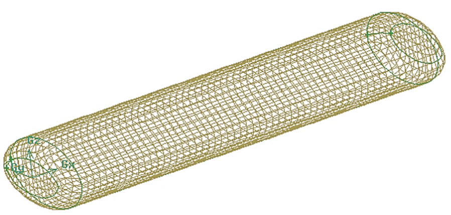
Modeling of tank using ANSYS Fluent.

Three oval cross-section sizes of tank were selected as shown in Table 2. The cross-section area is 0.147 m², and the liquid level ranges from 50% to 90%. Using the ANSYS Fluent software for simulation analysis, the liquid level was maintained at 50%, 60%, 70%, 80%, and 90%. Tank 1 was compared with the lateral sloshing force.

Table 2.

Oval tank size.

Tank size	Tank	Long axis (m)	Short axis (m)
The oval	Tank 1	0.260	0.175
	Tank 2	0.280	0.167
	Tank 3	0.300	0.156

If the initial surface is 15°; the lateral acceleration of the load on the tanks is

a_{y} = g \tan φ = 0.267 g

(41)

In formula (41), the lateral acceleration of the tank is 0267g. Under the external excitation, the liquid is forced to oscillate in the tank, impacting the tank wall. Under different liquid levels, the sloshing force contrast is shown in Figure 9.

Figure 9.

Lateral force variation with time: (a) fill level 50%, (b) fill level 60%, (c) fill level 70%, (d) fill level 80%, and (e) fill level 90%.

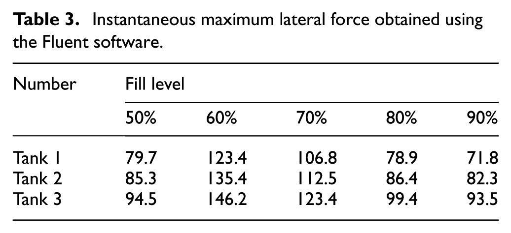
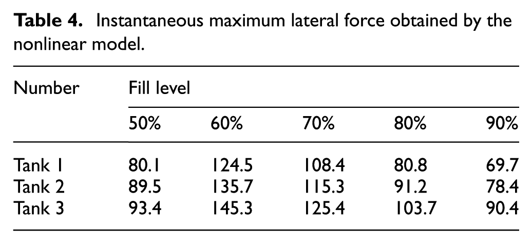
In Tanks 1–3, the liquid level ranges from 50% to 90%. The instantaneous maximum lateral force obtained using the Fluent software and nonlinear model is shown in Tables 3 and 4, and the relative deviation between them is shown in Figure 10(c).

Table 3.

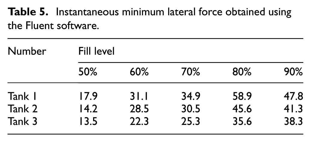
Instantaneous maximum lateral force obtained using the Fluent software.

Number	Fill level
Number	50%	60%	70%	80%	90%
Tank 1	79.7	123.4	106.8	78.9	71.8
Tank 2	85.3	135.4	112.5	86.4	82.3
Tank 3	94.5	146.2	123.4	99.4	93.5

Table 4.

Instantaneous maximum lateral force obtained by the nonlinear model.

Number	Fill level
Number	50%	60%	70%	80%	90%
Tank 1	80.1	124.5	108.4	80.8	69.7
Tank 2	89.5	135.7	115.3	91.2	78.4
Tank 3	93.4	145.3	125.4	103.7	90.4

Figure 10.

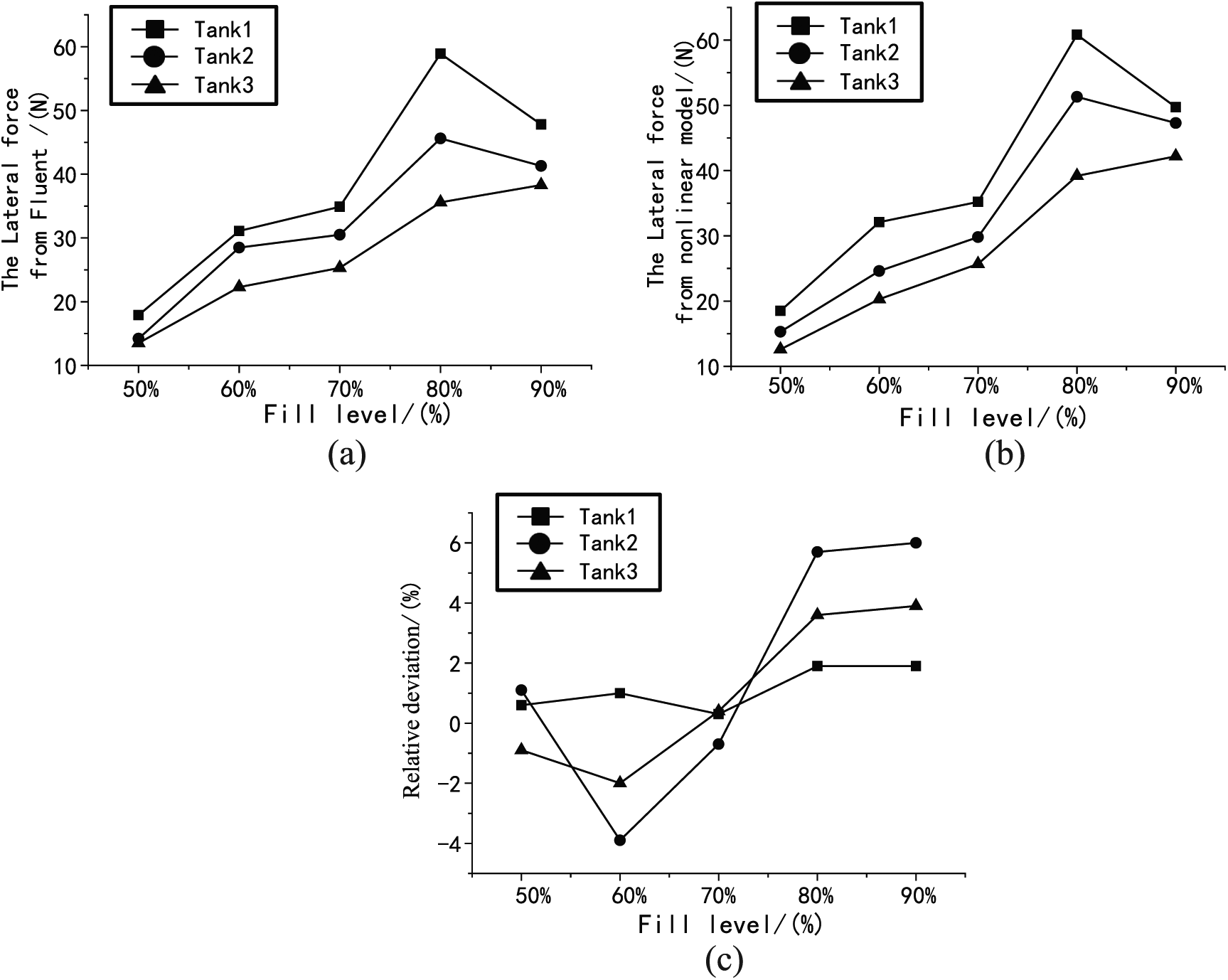
Instantaneous maximum lateral force: (a) Fluent, (b) model, and (c) relative deviation.

Figure 10(a) and (b) shows that the instantaneous maximum lateral force has the same trend for both the methods. When the liquid level is 60%, the instantaneous maximum lateral force is the maximum. With the increase in the liquid level, the instantaneous maximum lateral force decreased continuously. Figure 10(c) shows that the relative deviation between the two methods is within 5%.

In Tanks 1–3, the liquid level is from 50% to 90%. The instantaneous minimum lateral forces obtained using the Fluent software and nonlinear model are shown in Tables 5 and 6, and the relative deviation is shown in Figure 11(c).

Table 5.

Instantaneous minimum lateral force obtained using the Fluent software.

Number	Fill level
Number	50%	60%	70%	80%	90%
Tank 1	17.9	31.1	34.9	58.9	47.8
Tank 2	14.2	28.5	30.5	45.6	41.3
Tank 3	13.5	22.3	25.3	35.6	38.3

Table 6.

Instantaneous minimum lateral force obtained using the nonlinear model.

Number	Fill level
Number	50%	60%	70%	80%	90%
Tank 1	18.5	32.1	35.2	60.8	49.7
Tank 2	15.3	24.6	29.8	51.3	47.3
Tank 3	12.6	20.3	25.7	39.2	42.2

Figure 11.

Instantaneous minimum lateral force: (a) Fluent, (b) model, and (c) relative deviation.

Figure 11(a) and (b) shows that the instantaneous maximum lateral force has the same trend for both the methods. When the liquid level is 80%, the instantaneous minimum lateral force is the maximum. With the increase in the liquid level, the instantaneous maximum lateral force increases continuously. Figure 11(c) shows that the relative deviation between the two methods is within 7%.

Nonlinear pendulum model and simulated test bench analysis

The sloshing phenomenon of a tank liquid was studied using a simulated test bench. The results show that the test bench can better represent the liquid sloshing phenomenon in the tank; thus, it is an effective method to validate the numerical model. Therefore, the liquid sloshing nonlinear model was numerically simulated in this section, and the data of the simulation test bench were compared to evaluate the accuracy and applicability of the nonlinear model.

Under the working condition of simulated test to test data, the equivalent mechanical model was compared and analyzed. The dimensions of the oval cross section of tanks were as follows: a = 1.471 m and b = 1.387 m. The liquid level was 50%. The external excitation frequency was 1 Hz. The comparative data of lateral sloshing force are shown in Figure 12(a) and (b), and the relative deviation is shown in Figure 12(c). The data curves of the nonlinear dynamic model and test bench are almost the same; most of the relative deviation is less than 10%. Thus, the nonlinear dynamics model can well describe the nonlinear movement of liquid sloshing in a tank.

Figure 12.

Nonlinear model and comparison of simulated test: (a) nonlinear model, (b) simulated test bench, and (c) relative deviation.

Conclusion

The pendulum model was used to describe the liquid sloshing nonlinear phenomenon in a tank. Using Lagrange equation, a liquid sloshing pendulum under a nonlinear incentive model was established. The cycloid length and quality of pellets of the nonlinear pendulum model were determined. Using simulated test data, the nonlinear pendulum model was verified, and the lateral sloshing force data were obtained. The results show that when the liquid level is 90%, the instantaneous minimum lateral force is the minimum. Under the condition of liquid fill level, the liquid impact force in tank can be minimized. Therefore, it is suggested that the liquid fill level of tank truck is about 90%. The results also show that the most relative deviation is less than 10%, and the nonlinear pendulum model can more accurately describe the liquid lateral sloshing in a tank wall during the nonlinear dynamic phenomenon.

Footnotes

Handling Editor: Francesco Massi

Declaration of conflicting interests

The author(s) declared no potential conflicts of interest with respect to the research, authorship, and/or publication of this article.

Funding

The author(s) disclosed receipt of the following financial support for the research, authorship, and/or publication of this article: This study was supported by the Heilongjiang Province Science Foundation for Youths (QC2017040), The Fundamental Research Funds for the Central Universities (2572017BB01), and The Northeast Forestry University 5211 Special Funding (41112451).

ORCID iD

Jiangwei Chu

References

Abramson

Chu

Kana

. Some studies of nonlinear lateral sloshing in rigid containers. J Appl Mech 1966; 33: 777–784.

Abramson

. Representation of fuel sloshing in cylindrical tanks by an equivalent mechanical model. Arch Dermatol Syph 1961; 54: 491–492.

Zakaria

Osman

Saadun

MNA

et al . Computational simulation of boil-off gas formation inside liquefied natural gas tank using evaporation model in ANSYS fluent. Appl Mech Mater 2013; 393: 839–844.

Lee

. Stability and control of liquid propellant rocket systems. J Am Rocket Soc 2012; 23: 75–81.

Pinson

. Recent advances in structural dynamics of large space structures. Acta Astronaut 1989; 19: 161–170.

Miles

. Stability of forced oscillations of a spherical pendulum. J Acoust Soc Am 1962; 20: 21–32.

Miles

. Resonant motion of a spherical pendulum. Physica D 1984; 11: 309–323.

Miles

. The pendulum from Huygens Horologium to symmetry breaking and chaos—theoretical and applied mechanics. Theor Appl 1989; 1989: 193–215.

Georgia Institute of Technology. Office of sponsored programs. Analytical mechanical model for the description of the rotary propellant sloshing motion. Zamm J Appl Math Mech 1991; 71: 289–291.

10.

Bauer

Eidel

. Non-linear hydroelastic vibrations in rectangular containers. J Sound Vib 1988; 125: 93–114.

11.

Bauer

Siekmann

Wang

JTS

. Axisymmetric hydroelastic sloshing in an annular cylindrical container. J Spacecraft Rockets 1968; 5: 981–983.

12.

Abramson

. The dynamic behavior of liquids in moving containers. Appl Mech Rev 1966; 16: 501–506.

13.

Kana

. Vertical oscillation of partially full spherical tanks (SWRI NASw-146). San Antonio, TX: Southwest Research Institute, 1963.

14.

Unruh

Kana

Dodge

et al . Digital data analysis techniques for extraction of slosh model parameters. J Spacecraft Rockets 1986; 23: 171–177.

15.

Ikeda

Ibrahim

Harata

et al . Nonlinear liquid sloshing in a square tank subjected to obliquely horizontal excitation. J Fluid Mech 2012; 700: 304–328.

16.

Sankar

. Impact of dynamic fluid slosh loads on the directional response of tank vehicles. Veh Syst Dynam 1992; 21: 385–404.

17.

Ibrahim

Pilipchuk

Ikeda

. Recent advances in liquid sloshing dynamics. Appl Mech Rev 2001; 54: 133–199.

Computational simulation of nonlinear liquid sloshing in a tank truck

Abstract

Keywords

Introduction

Liquid pendulum sloshing model under nonlinear excitation

Parameters of nonlinear pendulum model

Determination of cycloid length of pendulum model

Determination of liquid sloshing quality on pendulum model

Analysis of the nonlinear pendulum model of liquid sloshing

Numerical simulation analysis of the nonlinear pendulum model

Comparison and analysis of nonlinear pendulum model with ANSYS Fluent

Nonlinear pendulum model and simulated test bench analysis

Conclusion

Footnotes

Declaration of conflicting interests

Funding

ORCID iD

References