
Abstract
This paper presents the robustness in formation control of multiple mobile robots using leader-follower method. The uncertainty considered is the measured error which is included in the relative state. The robust stability conditions against the relative state error are derived by Lyapunov’s stability theory (direct method). We also obtain the formation steady-state deviation when formation stability is ensured. The formation control environment is constructed on Simulink. The validity of the stability condition and the steady-state deviation is demonstrated by numerical simulation. It is seen that the L-F method provides a robust control law against the relative state error although large formation steady-state deviation is occurred in some cases.
Introduction
Formation control of multi-mobile robots has attracted much attention in recent years. In this background, the formation is one of efficient transportation forms such as automobiles and airplanes, and it can become a system that brings about more efficient work achievement than a single robot.1–4 Reactive behavior-based method,5–7 multi-agent system method,8–11 virtual structural method,12,13 and leader-follower (L-F) method14–18 are well known as control approaches to realize formation control. This paper is a study on the L-F method for mobile robots. In this method, multiple mobile robots are classified into a leader and followers. The objective of the leader is to lead the fleet of the followers, while that of the followers is to keep the specified relative positional relation with the leader. Therefore, the issue to be examined in the L-F method is basically to design control systems for the followers.
The authors have been studying several issues in formation control based on the L-F method by using real mobile robots; autonomous decentralized control law, obstacle avoidance, and shape transition.19–23 The control system designs were based on feedback linearizaton.24,25 The parameters of the control law were given while checking real operation status of the mobile robots. Since the decentralized control law19,21 was constructed by the relative states; that is, the relative distance and the relative angle, which were measured by the followers, the relative states included the measured errors. Fortunately, the designed control law was acceptable without troubles in carrying out the experiments mentioned above. However, the control system of the L-F method is a nonlinear system with respect to the relative states, and the relative state errors may have influences on the stability and the control performance of the closed-loop system. The L-F method is one of the well-known control methods not only for mobile robots but also for UMV/UAV formation control such as multi-rotor vehicles.26–28 However, there are few researches for investigating the robustness against the relative state errors. It is therefore worth verifying the robustness of the L-F method.
This paper discusses the robustness in the formation control of mobile robots using the L-F method. First, the problem setting of formation control considered in this paper is clearly defined. Since the L-F method treats the kinematics of mobile robots, the uncertainty in the controlled system is the measured error which is included in the relative state. This paper derives the stability conditions based on Lyapunov’s stability theory29,30 for the closed-loop system with the relative state errors containing control law. The steady-state deviation in formation control is presented when the stability is ensured. Its approximate representations are also derived. The formation control environment is constructed on Simulink. The validity of the stability condition and the steady-state deviation is demonstrated by numerical simulations. Through these analysis and simulation, this paper provides the effectiveness and the robustness of the L-F method from the theoretical point of view.
Leader-follower method of mobile robots
Statements of problem
Let us consider a mobile robot with nonholonomic constraints. The position of a robot moving in a two-dimensional plane is represented by a stationary Cartesian coordinate system


Where


Relative position and relative orientation between leader and follower robot.
To make the formation control issue of mobile robots clear, this paper defines application policies of the L-F method as follows.
(M-1) Multiple mobile robots with nonholonomic constraints form a formation in the forward direction.
(M-2) The leader is used to lead the fleet of the followers to the target, while the followers follow the leader with keeping the relative positional relation specified in advance.
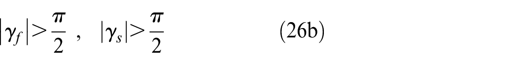
(M-3) The formation trajectory, also called the leader trajectory, is given by a trajectory with a smaller limit on the relative azimuth
(M-4) The transitional velocity of the leader vl is given within the specified range.
Based on these application policies, the objective of the formation control in this paper is that the followers are controlled by their translational and the angular velocities vf and ωf so as to keep the relative states
Relative state-space equation
The kinematics of a mobile robot is given by the following equation.

When differentiating both sides of equations (1) and (2) by t and using equation (6) corresponding to the leader and the follower, the derivatives of the relative distance and angle of the follower can be expressed collectively as.19,20


Equation (7) is called the relative state-space equation, which means the controlled object in this paper. The control objective described in the previous section is to design the control input of the follower ηf which achieves ξf→ξf ref for t→∞ in equation (7). The control input by feedback linearization is given as follows.


µf is a linear input whose gain matrix K is given by
Equation (9a) is used to cancel out the nonlinear terms in equation (7). However, when

This achieves the control objective ξf→ξf ref when t→∞.
Relative state-space equation with relative state error
To use the control input (9a), the follower needs to measure the relative distance and angle by its own sensor. Denoting these measurements as ds and
εd and εγ are called the relative distance and the relative angle errors, respectively. For convenience in the following descriptions, the following vector notations are used collectively as the relative state error and the measured relative state.

When the relative state error ef is contained in ξf , the control inputs by feedback linearization are given by

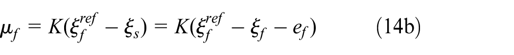
Equation (14a) is not constructed when

Equation (15) shows the closed-loop system with the relative state error. In the following sections, we will discuss the stability of the closed-loop system and the steady-state deviation when it is stable. Equations (12a) and (12b) are generally time-varying, but in this paper, we consider a case that they are constant. Note that the equilibrium point of equation (15) is the relative state whose derivative is equal to zero; that is,
Stability condition with relative state error
This section presents a stability condition for the closed-loop system with the relative state error by using Lyapunov’s stability theory (direct method).29,30 Since the range of the relative state should be taken into consideration (see Section “Range of relative state”), the stability condition to be derived in this section is the local asymptotic stability. At the beginning, the following variable transformation

is applied to equation (15). The closed-loop system (15) is then rewritten as follows.


By equation (16), the equilibrium point is moved to the origin (z eq = 0). The last notation of equation (18) is used for Lyapunov equation which will be presented in Section “Lyapunov equation with respect to Acl(z).”g(z;du) in equation (19) satisfies the following constraints:


Equation (20a) is obvious from the definition of the equilibrium point ξf eq . Equation (20b) is a constraint on the magnitude of g(z;du), where cg may be constant or varying (see Section “Verification by simulation”).
Range of relative state
The range of the relative state should be taken into consideration in the formation control from the viewpoints of the definition of the variables, the constraints on the control law and the practical application. As for the relative distance df , it is a positive number from the definition. There exists an upper limit due to the distance sensor. There also exits a lower limit for avoiding collisions between robots. As for the relative angle
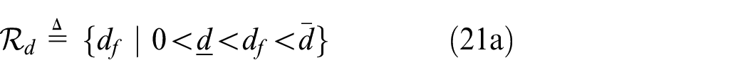

Where
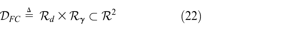
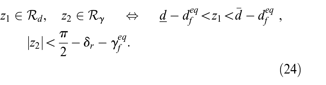
is defined as the formation region. Thus,

This is also used for the transformed variable z. That is,
Lyapunov equation with respect to Acl(z)
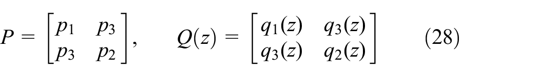
As a preparation for applying Lyapunov’s stability theory to equation (17), the following Lyapunov equation

is introduced in this section, where P is a constant matrix and Q(z) is a z-dependent matrix. They are positive definite. For existence of a unique solution in equation (25), Acl(z) must be a stable matrix. Eigenvalues of Acl(z) are

or
is satisfied, Acl(z) is a stability matrix. Then, the existence of Lyapunov equation (25) is expressed in the following theorem.

where α and
Proof. When P and Q(z) defined as
are used in equation (25), the following relationship is obtained.

When some elements of P and Q(z) are given as

the rest of the elements are obtained as

Thus, equation (27) is obtained. Furthermore, P > 0 because of α,

for α,
Equation (26a) is suitable for (M-1) and (M-2), whereas equation (26b) is not. Equation (26a) also corresponds to
Stability condition
The following is a stability condition which is obtained by applying Lyapunov’s stability theory to the closed-loop system (17).
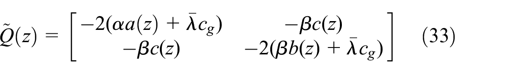
is positive definite, where
Proof. Using equations (17), (20b), and (25), the derivative of V (z) is
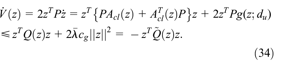
Thus, if
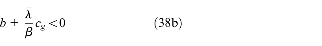
Theorem 2 expresses the stability condition of the closed-loop system (17) as
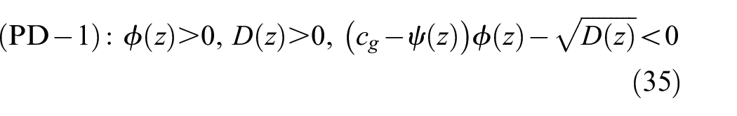

where

Proof. The necessary and sufficient condition for


(i)


ζ which the left-hand side of equation (39c) becomes zero is given by

When D ≤ 0, there is no ζ satisfying equation (39c). When D > 0, it exists in the range of

For existence of ζ ≥ 1, ζ1 has to be greater than one. To summarize the above, the conditions for
(ii)


ζ satisfying equation (42c) is given by
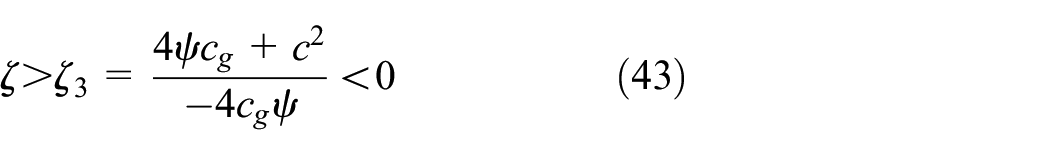
For existence of ζ < 1, ζ3 has to be smaller than one. To summarize the above, the conditions for
Equations (38a) and (38b) are redundant in the condition of
Steady-state deviation in formation control
This section presents evaluation of the steady-state deviation when the relative state error ef is included. As the leader trajectory is given according to (M-3) and (M-4), this paper deals with a case where ef and du are constant.
Formation steady-state deviation (FSSD)
In the formation control, the following deviations are defined.


Δξf (t) and Δξs(t) are called true and virtual formation deviations, respectively. The latter is known and is used in the linear input (14b) µf = KΔξs. Both deviations are related as

These steady-state deviations, taken as t→∞, are written as follows.


Δξf
ss
and Δξs
ss
are the true and the virtual formation steady-state deviations (FSSDs), respectively. In equation (15) for the case of the leader trajectory with constant du, they are expressed by the following equations by

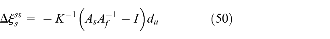
where the relative states included in the elements of As and Af in equation (50) are the steady-state when t→∞. Equation (49) means that the true FSSD is the sum of the relative state error and the virtual FSSD. Using equations (4), (8), and (18), the elements of Δξs ss are derived as follows:
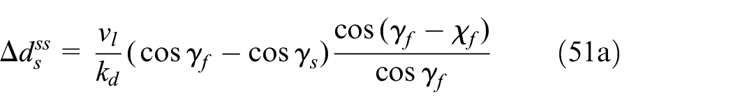

where all of the relative states in the above equations are the steady-state when t→∞.
Approximation of virtual FSSD
This section presents two approximations to simplify virtual FSSD.
Approximation 1. For the leader trajectories that satisfy (M-3), the following approximation holds.

Using this into equations (51a) and (51b), the virtual FSSD is approximated as

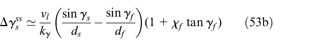
Approximation 2. For the leader trajectories that satisfy (M-3) and smaller relative state error,


the following approximation also holds.
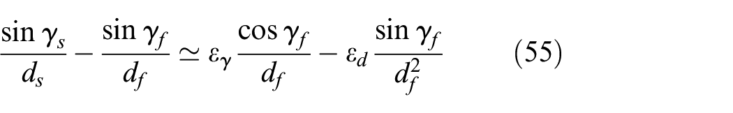
Using this into equations (53a) and (53b), the virtual FSSD is approximated as
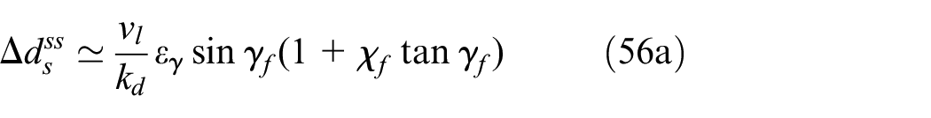

These two approximations provide the following considerations for the virtual FSSD. Δds ss and Δγs ss are proportional to vl and inversely proportional to kd and kγ. The relative angle error εγ affects both Δds ss and Δγs ss proportionally. On the other hand, the relative distance error εd affects Δγs ss but not Δds ss because it is not explicitly included.
Verification by simulation
This section presents simulation results in which formation control by a leader and two followers, referred to as L, F1, and F2 hereafter, was performed on Simulink. Since the purpose of this simulation was to confirm the stability conditions and the FSSDs derived in Sections “Stability condition with relative state error” and “Steady-state deviation in formation control,” the results for typical cases are presented, rather than simulations for all cases. Therefore, more detailed studies, such as the boundary of stability range and techniques to improve the FSSD, are left to the other reports in future. The simulation conditions are shown below.
Leader trajectory
Straight line on x-axis with constant velocity vl = 2 [m/s]
Formation shape and referenced relative states

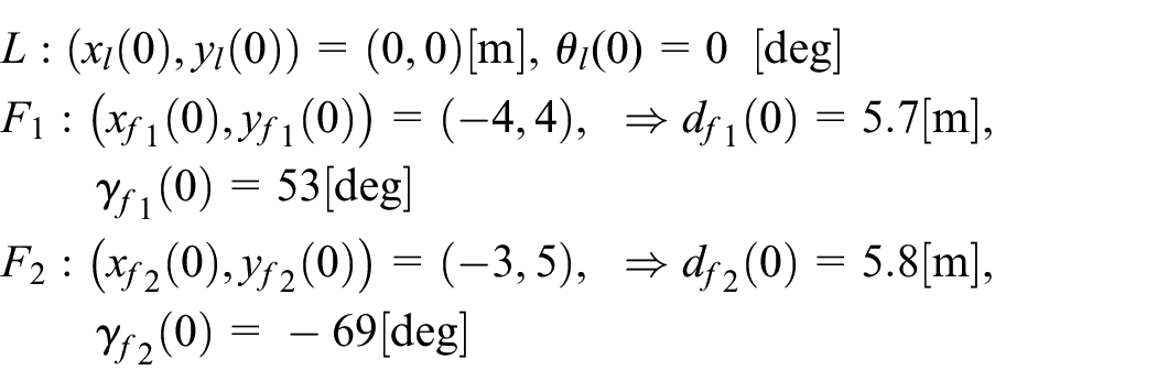
Initial position and azimuth
Constraints on control input

Gain of linear input

Relative state errors

Parameter values in the formation region

Some explanations are given on the above condition setting. The leader trajectory was given by a straight line (referred as Line hereafter) on x-axis with a constant velocity as a simple setting. Formation shape was given by a triangle. As for the initial position of the mobile robots, L was placed at the origin and faced to the direction of x > 0. F1 and F2 were placed at the appropriate coordinates and directions. The linear input gain was the same for F1 and F2. It was assumed that the relative state errors εd and εγ were only added to F1 within the specified ranges shown above. Thus, the control law for F1 was equation (14), whereas that for F2 was equation (9). Since F2 was always formation stable and the FSSD was consistently zero, the simulation results shown below will be the stability and the FSSD of F1. Furthermore, since the simulation here was to examine the robustness, the constraints of the control input were not imposed. The formation region
Formation stability
Table 1 summarizes the formation stability when constant relative state errors εd and εγ were included in the control law of F1. In these tables, “S” means formation stable and “Un” means unstable. The relative state errors examined were equivalent to the referenced relative states from 10% to 70%. However, the closed-loop system was formation stable for wide ranges of the relative state errors.
Formation stability region of F1 with respect to relative state errors.

Table 2 shows the details of six typical cases with respect to the formation stability. “Cond. of Theorem 3” shows the conditions of Theorem 3, where cg in equation (20b) was examined by the following two cases; 1: cg = max(||g(z; du)||/||z||) (constant) and 2: cg = ||g(z; du)||/||z|| (varying). “⊙” means that (PD-1) or (PD-2) was satisfied over the entire simulated time-range, “
Summary of typical cases with respect to formation stability of F1.


Time histories in straight line formation, Case A (εd = 0.4 [m], εγ = −20 [deg]): (a) trajectory of L, F1, and F2 and (b) condition of Theorem 3, cg: 1.

Time histories in straight line formation, Case C (εd = 1.4 [m], εγ = −20 [deg]): (a) trajectory of L, F1, and F2 and (b) condition of Theorem 3, cg: 2.

Time histories in straight line formation, Case E (εd = 0.8 [m], εγ = 10 [deg]): (a) trajectory of L, F1, and F2, (b) relative state, and (c) control input.
In Cases A and B, a(z) which is one of the eigenvalues of Acl was negative over the entire simulated time-range, and there existed a Lyapunov solution P. In Case A, both (PD-1) and (PD-2) of Theorem 3 were satisfied. The equilibrium point was locally asymptotically stable (Figure 2(b)). By “cg: 1” in Case B, it was not satisfied in the latter half of the simulation. In “cg: 2,” on the other hand, (PD-1) was not temporarily satisfied, but was almost satisfied. The constraint of “cg: 1” was more conservative than that of “cg: 2.”
In Cases C, D, and E, a(z) was partly positive and neither (PD-1) nor (PD-2) was satisfied in the latter half of the simulation. The closed-loop system was formation stable in Case C but unstable in Cases D and E. This depended on whether
Summarizing the above discussion of the formation stability, the closed-loop system of the formation control by the L-F method was able to ensure the formation stability even for relatively large relative state errors. In particular, when (PD-1) or (PD-2) in Theorem 3 was satisfied, the L-F method guarantees the formation stability and achieves allowable formation performance along with the application policies. Moreover, when the relative angle was near the singular point of the control law and the measured initial relative angle was outside of
FSSD
Figure 5 shows the FSSD with respect to the relative state error εd and εγ. The dotted-squares in the figures are

FSSD of F1: (a) virtual FSSD of relative distance, (b) true FSSD of relative distance, (c) virtual FSSD of relative angle, and (d) true FSSD of relative angle.
Since the leader trajectory in this simulation was a straight line, Approximation 1 given by equation (53) was consistent with equation (51). Table 3 shows the range of the virtual FSSD given by equations (51) and (56) (Approximation 2). It is seen that Approximation 2 was acceptable in the region of “small relative state error.”
Range of virtual FSSD given by equations (51) and (56) (Approximation 2) within “small relative state error”: |εd| ≤ 0.4 [m] and |εγ| ≤ 20 [deg].

Summarizing the above discussion, the true FSSD was caused by the relative state error and the virtual FSSD derived from the leader’s state. εd did not affect both
Further simulations
To enhance the validity of the stability condition and the formation steady-state deviation, which were described in Sections “Stability condition with relative state error” and “Steady-state deviation in formation control,” this section presents the following additional simulations: sinusoidal leader trajectory (referred as Sinusoid hereafter) and five follower formation.
Sinusoid formation
Figures 6 to 8 show the time histories in sinusoid formation where the relative errors were given by Cases A, C, and E in Table 2. As shown in the figures, Cases A and C were formation stable but Case E was unstable. The results shown in Figures 6 to 8 were approximately similar to those in Figures 2 to 4 in which the leader trajectory was given by a straight line. Thus, as mentioned in Section “Formation stability,” the conditions of Theorem 3, the equilibrium and the initial of the relative angle were closely related to the formation stability.

Time histories in sinusoid formation, Case A (εd = 0.4 [m], εγ = −20 [deg]): (a) trajectory of L, F1, and F2 and (b) condition of Theorem 3, cg: 1.

Time histories in sinusoid formation, Case C (εd = 1.4 [m], εγ = −20 [deg]): (a) trajectory of L, F1, and F2 and (b) condition of Theorem 3, cg: 2.

Time histories in sinusoid formation, Case E (εd = 0.8 [m], εγ = 10 [deg]): (a) trajectory of L, F1, and F2, (b) relative state, and (c) control input.
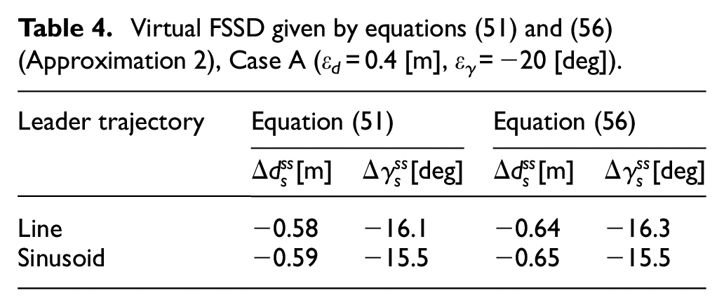
Table 4 shows the virtual FSSD given by equations (51) and (56) (Approximation 2), where the relative state error was Case A which was within the region of “small relative state error.” The leader trajectory was given by Line and Sinusoid. It is seen that Approximation 2 was acceptable in both leader trajectories.
Virtual FSSD given by equations (51) and (56) (Approximation 2), Case A (εd = 0.4 [m], εγ = −20 [deg]).
Five follower formation
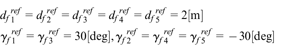
This section presents a formation control where the number of the followers was five. The formation shape was given by a triangle structure which is shown in Figure 9. The references of the followers were given as

Structure of five follower formation.
The leader for F1 and F2 was L, the one for F3 and F4 was F1 and the one for F5 was F2. The orange dashed-line in Figure 9 indicates that the measured relative states of F1, F3, and F5 included the following relative state errors:

Figure 10 shows the trajectory of five follower formation where the leader trajectory was given by Line. Although some FSSDs occurred, the formation stability was established by satisfying the stable conditions between each leader and follower.

Trajectory of five follower formation, Line.
As mentioned above, it is concluded from further simulations that the stability conditions and the FSSD described in Sections “Stability condition with relative state error” and “Steady-state deviation in formation control” were also effective in curved leader trajectory and increase of the followers.
Concluding remarks
This paper has presented the robustness of the formation control of mobile robots using the L-F method. The uncertainty considered was the relative state error which was included in the relative state. The robust stability conditions against the relative state error were derived by Lyapunov’s stability theory (direct method). We also obtained the formation steady-state deviation (FSSD) when the formation stability was ensured. The formation control environment was constructed on Simulink. The validity of the stability condition and the FSSD was demonstrated by numerical simulation. Consequently, it was seen that the closed-loop system was formation stable even for large relative state error; that is, the L-F method provided a robust control law against the relative state error. On the other hand, for the FSSD, the validity of the derived approximation was shown in the region in which the relative state errors were small. These results were similar to those obtained in which the leader trajectory is curved and the number of followers was increased. However, large FSSD was occurred in some cases although it was formation stable. These cases should be avoided in practical application. Some techniques are required to reduce the large FSSD.
The knowledge obtained in this paper clarified that the L-F method has robust characteristics from a theoretical point of view, and it may be said that we showed the superiority of using the L-F method for formation control. This paper considered the relation of one leader and one follower. When the number of followers is increased in the L-F method, the formation is developed by constructing the relation of leader and follower continually, and the control law is installed on each follower in the decentralized control approach. Therefore, the robust stability and the FSSD presented in this paper are effective in each relation of leader and follower. This was demonstrated in further simulations.
Since the simulation presented in this paper was the examination in the case of constant relative state error, it is required to obtain more enough knowledge by varying relative state error. Furthermore, it seems to be necessary for the practical application of the L-F method to examine a reduction technique on the FSSD. These are future research subjects.
Footnotes
Handling Editor: Chenhui Liang
Declaration of conflicting interests
The author(s) declared no potential conflicts of interest with respect to the research, authorship, and/or publication of this article.
Funding
The author(s) received no financial support for the research, authorship, and/or publication of this article.