Analytical modeling and experimental verification of churning torque for cam guide rails of 2D piston pump

Abstract

For 2D piston pump the churning torque of its cam guide rails at high speed is one of the main sources of mechanical efficiency loss. To conveniently calculate the churning torque and also provide guidance for future optimization of churning torque reduction, an accurate analytical model of constant acceleration and constant deceleration cam guide rail assembly of the stacked-rollers 2D piston pump is established, where the whole churning torque is divided into the peripheral churning torque, the pushing flow churning torque, and the end face churning torque. Then the analytical model is verified by CFD simulation preliminarily. Analytical modeling shows that at 16,000 rpm, the churning torque reaches about 0.826 N m, where the peripheral churning torque, the pushing flow churning torque, and the end face churning torque account for about 55.4%, 37.3%, and 7.3% of the total torque respectively, indicating that the structural parameters related to the pushing flow torque should be optimized with first priority at high rotational speed. Finally, the churning torque at 1000–16,000 rpm was experimentally measured and the influence of oil temperature was considered. The experimental results are in good agreement with the results of analytical modeling and CFD simulation, thus verifying the correctness of the proposed analytical model.

Introduction

The hydraulic pump is the “heart” of the hydraulic system, and the axial piston pump is widely used in aviation hydraulic systems because of its compact structure, high pressure, and large displacement.^1–3 For the modern high speed electrical motor, it is easier to increase the speed than to increase the output torque. Therefore, increasing the speed has become the main breakthrough for improving the power density of the aviation axial piston pump.^4,5 However, when the pump is working, the piston, cylinder block, and other components are immersed in hydraulic oil, which results in churning loss.

The energy loss of the axial piston pump is an important factor affecting its power density, which can be divided into mechanical loss, volume loss, and churning loss. The speed requirements of hydraulic pumps used in industrial hydraulics and mobile machinery are usually lower than 3000 rpm, and the oil churning loss is not obvious The proportion of churning loss increases rapidly as rotational speed increases, which becomes one of the main factors restricting the power density of axial piston pump. ⁶ Therefore, the churning loss of axial piston pump drawn attention of the scholars. Jang ⁷ emphasized the piston’s rotary motion is an important factor affecting the churning loss in the axial piston pump. Zecchi et al. ⁸ considered the churning loss of the cylinder and the piston in the energy loss firstly, and established a corresponding analytical model. Olsson ⁹  measured the churning loss during the actual operation of the axial piston pump, and estimated that churning loss accounted for 15%−20% of the energy loss. Xu et al. ¹⁰  established a coupled simulation model of churning loss, and found that the oil flow state inside the piston pump changed from laminar flow to turbulent flow, and the pressure resistance loss increased significantly. Zhang et al.^11,12 researched the churning loss of the cylinder and piston assembly respectively, and found that when the speed exceeds the critical speed, the churning loss of the piston is smaller than that of the cylinder. Li et al. studied how the number of pistons affects churning loss based on CFD simulation. The results show that under the same displacement, the churning loss of seven pistons is greater than that of nine pistons. When the number of pistons and the displacement of the pistons are the same, reducing the pitch radius of the piston hole is the best method to reduce the churning loss. ¹³ Wei et al. used the moving particle semi-implicit (MPS) method to calculate the churning loss of the hydraulic pump, and the results showed that the total churning loss decreased with the decrease of the tilt angle of the swash plate. When the oil content is 70%, the churning loss of the pump is reduced by 57.4%. ¹⁴ There are also structural improvements to decrease the oil churning loss of the pump rotational components. Parker company added a power booster unit to the hydraulic motor, ¹⁵ Danfoss company invented a dry bending shaft motor. ¹⁶ And Chao et al. ¹⁷  established a mathematical model to analyze the churning loss of the axial piston pump, it provides a basis for accurately calculating the churning loss of the high-speed axial piston pump. Ding et al.^18,19 studied the churning loss of a force-balanced 2D pump at high speed through CFD simulations and experiments.

The above review reveals that 3D CFD numerical simulation based on moving mesh is still the mainstream method in the research process of churning loss. However, CFD simulations are time-consuming and labor-intensive, it often measured in days to make computation with millions of meshes at every turn. In addition, if the structural parameters of the hydraulic pump are modified, then its CAD model and CFD simulation model need to be modified at the same time. Therefore, the method of CFD simulation is also difficult to quickly realize the optimal design of structural parameters for the purpose of reducing the churning loss. On the contrary, the analytical modeling method is convenient and fast to calculate, and it can clearly reveal the influence of key structural parameters on churning loss. However, the internal flow field of the axial piston pump is relatively complex, and it is quite difficult to establish an accurate analytical model.

Since the three sliding friction pairs of the axial piston pump are based on oil film support, the working conditions are poor during variable speed and emergency start and stop. In recent years, rolling supports have also replaced sliding friction pairs to form high-speed piston pumps with new structural principles. The novel 2D piston pump proposed by Ruan et al.^20–22 is a typical representative. Compared with the traditional axial piston pump, the 2D pump uses the rolling support based on cam guide rail to replace the sliding support of swash plate slipper to realize the oil suction and drainage of the piston cavity, and uses the piston flow distribution to replace the original flow distribution plate, which greatly simplifies the design of the axial piston pump. Its highly integrated structure is naturally suitable for aviation hydraulic systems.^23–25 For 2D pump, cam guide is the core mechanism to realize the functions of oil suction and discharge and flow distribution since its shape curve determines the reciprocating motion law of the piston, and even affects the performance parameters of the whole pump, such as load, pressure pulsation, flow pulsation, etc. As the most important moving components, the cam guide rails are also immersed in oil when they work. The rotation of the guide rail at high speed is the main source of the churning loss of the 2D piston pump. Therefore, it is of great theoretical significance and practical engineering meaning to study it.

To conveniently calculate the churning torque and also provide guidance for future optimization of churning torque reduction, an accurate analytical model of constant acceleration and constant deceleration cam guide rail assembly of the stacked-rollers 2D piston pump^26,27 is established, and experimental verification is carried out. The remaining of this paper is structured as follows: In section “Structure and operating principle,” the structure and operating principle of the stacked-rollers 2D piston pump is introduced briefly. In section “Analytical modeling,” an accurate analytical model of churning torque is established based on the fundamentals of fluid mechanics, where the whole churning torque is divided into the peripheral churning torque, the pushing flow churning torque, and the end face churning torque. In section “CFD numerical simulation,” the accuracy of the analytical model is verified based on CFD numerical simulation. And structural parameters optimization related to the pushing flow torque is discussed in detail. In section “Experiments and discussions,” the churning prototype is designed and machined, and the churning torque is measured on a special churning test rig. Then the experimental results, simulation results, and analytical results are analyzed and compared. Finally, some useful conclusion is drawn.

Structure and operating principle

The stacked-rollers 2D piston pump, as shown in Figure 1(a), consists of a transmission module as well as an oil suction and discharge module. A transmission shaft, cone rollers, a driving guide rail set, and a balancing guide rail set comprise the transmission module. The oil suction and discharge module is made up of a 2D piston, piston rings, an oil suction and discharge port, and a distribution cylinder. The driving guide rail set and balancing guide rail set are shown in Figure 1(b) and (c), respectively.

Figure 1.

The structure of stacked-rollers 2D piston pump: (a) stacked-rollers 2D piston pump, (b) driving guide rail set, and (c) balancing guide rail set.^26,27

Figure 2 shows the operating principle of the stacked-rollers 2D piston pump. The red marked area in the figure represents the oil under high pressure, and the blue marked area represents the oil under low pressure. During the operating process, the two guide rail sets rotate synchronously with the transmission shaft. Since the two guide rail groups are constrained by the cone roller group, the two guide rail groups realize linear axial reciprocating motion, which in turn makes the volume of the closed cavity change periodically to realize oil suction and discharge. The rotational angle marked in Figure 2 is 0°. At the moment, the piston and the piston ring is located at the far left end and the right end respectively, thus, and the left cavity has the largest volume. When the piston is rotated from 0° to 18°, the left cavity distribution groove connects to the oil discharge port and begins to discharge oil. The left cavity’s volume starts to decrease at this point, and at the same time, the distribution groove of the right cavity connects to the oil suction port to absorb oil, and the right cavity’s volume expands. When rotational to 72°, the 2D pump completes a cycle of oil suction and discharge. Therefore, the guide rail group rotates 360°, and the stacked-rollers 2D piston pump performs five times of oil suction and discharge.

Figure 2.

The operating principle of the stacked-rollers 2D piston pump.

Analytical modeling

Figure 3 represents the churning loss of the stacked-rollers 2D piston pump caused by the resistance of the oil when the guide rail rotates with high speed immersed into the oil. Taking the left guide rail assembly as an example, the churning torque of the stacked-rollers 2D piston pump is studied in detail.

Figure 3.

Guide rail assembly.

Based on fundamentals of fluid mechanics, the churning losses can be divided into two categories. One is the shearing action of oil between the moving component’s outer surface and the house’s inner wall. Due to the oil viscosity, when oil is sheared and deformed, an internal friction force that retards the deformation will be generated, resulting in a viscous friction torque. According to the different position of the viscous friction torque, the theoretical formula used is also different, so in this paper it is further divided into end face frictional force and peripheral frictional force. The other is the pressure difference resistance force. This is mainly because of the shape of the object that causes the pressure difference between the front and back of the object, which can also be denoted as pushing flow churning torque. Figure 4 gives the whole analytical modeling flow chart, where the total churning torque is divided into the peripheral churning torque, the pushing flow churning torque, and the end face churning torque.

Figure 4.

Flow chart of analytical modeling of oil churning torque.

End face churning torque

In this section, the end face churning torque is analytically modeled. Figure 5 shows the geometric parameters of the cam guide rail end face, where the brown part represents the large guide rail, and the yellow part represents the small guide rail. For convenience of calculation, the whole end face is deliberately divided into four zones, where the large guide rail is divided into zone 1, 2, and 3 and the small one occupies zone 4.

Figure 5.

Schematic diagram of geometric parameters of guide rail end face.

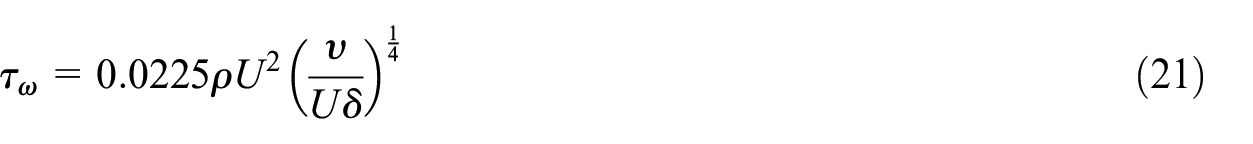
Firstly, the flow state near the end face can be determined by the Reynolds number formula. ²⁸

$$\mathrm{Re}=\frac{\rho \omega R^2}{\mu }\{\begin{array}{c}<{10}^5\mathrm{Laminar}\mathrm{flow}\hfill \\ \multicolumn{1}{c}{>3\times {10}^5\mathrm{Turbulent}\mathrm{flow}}\end{array}$$

(1)

where R represents radius, and ωR represents the rotational speed of end face edge of guide rail.

For laminar flow, on the fluid in the boundary layer with a distance from the rotation axis r, the centrifugal force per unit volume is equal to prω². Therefore, for the volume where the area is dr·ds and the height is δ, the centrifugal force is equal to ρrω²δdrds. The same fluid particle is also subjected to shear stress τ_ω, where τ_ω is opposite to the sliding direction of the fluid with an angle γ to the circumferential velocity. Thus, the radial component of τ_ω must be equal to the centrifugal force, which yields

$${\tau }_{\omega }\sin \gamma \mathrm{drds}=\rho r{\omega }^2\delta \mathrm{drds}$$

(2)

On the other hand, the circumferential component of the τ_ω must be proportional to the circumferential velocity gradient on the wall. It yields

$${\tau }_{\omega }\cos \theta ~\mu r\omega /\delta$$

(3)

τ_ω can be eliminated by combining the above two formulas, which yields

$${\delta }^2~\frac{\upsilon }{\omega }\tan \gamma$$

(4)

where υ is kinematic viscosity of fluid.

The thickness of the boundary layer induced by the churning of end face of the guide rail can be written as

$$\delta ~\sqrt{\frac{\upsilon }{\omega }}$$

(5)

Now calculate the viscous frictional torque on the end face of the guide rail. At the circular end face with radius of r and width of dr, the torque of a micro-element can be expressed as

$$\mathrm{dM}=-2\pi \mathrm{rdr}·r·{\tau }_{\omega }$$

(6)

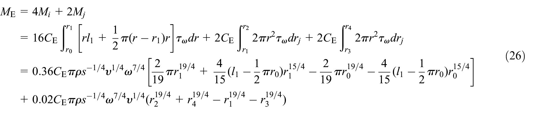
Therefore, for the end face of the guide rail wetted on single side, the torque can be expressed as

$$M=-2\pi {\int }_0^R{r}^2{\tau }_{\omega }\mathrm{dr}$$

(7)

$${\tau }_{\omega }=\mu {\left(\frac{\mathrm{dU}}{\mathrm{dz}}\right)}_{z=0}$$

(8)

where

$$U=r\omega G(\epsilon )$$

(9)

Here, G(ε) and ε are the dimensionless variables.

$$\epsilon =z/\delta =z\sqrt{\frac{\omega }{\upsilon }}$$

(10)

Combining formulas (8) and (9), the circumferential shear stress at the distance from the shaft r can be written as

$${\tau }_{\omega }=\rho r{\upsilon }^{\frac{1}{2}}{\omega }^{\frac{3}{2}}{G}^{\prime }(0)$$

(11)

where G’(0) = 0.616.

Substituting formula (11) into formula (7), the viscous torque of the end face of the unilateral guide rail can be written as

$$M=0.616\pi \rho R^4(\upsilon {\omega }^3{)}^{\frac{1}{2}}$$

(12)

The premise of the above calculation is that the distance s between the stationary wall and the rotational end face is larger than the thickness of the boundary layer δ. However, when s is smaller than δ, the change of tangential velocity across the gap should be as linear as the Couette flow. ²⁸ Thus, the circumferential shear stress at the distance from the shaft r can be rewritten as:

$${\tau }_{\omega }=\mu {\left(\frac{\mathrm{dU}}{\mathrm{dz}}\right)}_{z=0}=\mu r\omega /s$$

(13)

The calculation formula of boundary layer thickness near the lower end of laminar flow can be written as ²⁹

$$\delta \approx 5\sqrt{\frac{\upsilon }{\omega }}$$

(14)

Then the churning torque of the end face of the unilateral guide rail can be written as

$$M=2\pi {\int }_0^R{\tau }_{\omega }{r}^2\mathrm{dr}=\frac{\mu \pi \omega R^4}{2s}$$

(15)

Referring to the formulas (8) and (11), when s is larger than δ, for the guide rail end face wetted on single side, the viscous torque of ring i can be written as

$$\begin{array}{c}\multicolumn{1}{c}{M_i=4C_{\mathrm{E}}{\int }_{r_0}^{r_1}[r{l}_1+\frac{1}{4}\times 2\pi (r-r_0)r]{\tau }_{\omega }\mathrm{dr}=2.464C_{\mathrm{E}}{\int }_{r_0}^{r_1}[\frac{1}{2}\pi r^3+(l_1-\frac{1}{2}\pi r_0)r^2]\rho {\upsilon }^{1/2}{\omega }^{3/2}\mathrm{dr}}\\ =2.464C_{\mathrm{E}}\rho {\upsilon }^{1/2}{\omega }^{3/2}[\frac{1}{8}\pi r_1^4+\frac{1}{3}(l_1-\frac{1}{2}\pi r_0)r_1^3-\frac{1}{8}\pi r_0^4-\frac{1}{3}(l_1-\frac{1}{2}\pi r_0)r_0^3]\hfill \end{array}$$

(16)

where C_E is a correction coefficient. Considering that the end face shape of the guide rail is not a complete circle, the surrounding flow field will bring certain deviation to the analytical modeling results, so it is necessary to add C_E to the end face churning torque calculation. C_E could be obtained by the CFD simulated and analytical results of the end face churning torque.

Similarly, the viscous torque of ring j can be written as

$$\begin{array}{c}\multicolumn{1}{c}{M_j=C_{\mathrm{E}}{\int }_{r_1}^{r_2}2\pi r^2{\tau }_{\omega }d{r}_j+C_{\mathrm{E}}{\int }_{r_3}^{r_4}2\pi r^2{\tau }_{\omega }d{r}_j}\\ =0.616C_{\mathrm{E}}{\int }_{r_1}^{r_2}2\pi \rho r^3{\upsilon }^{1/2}{\omega }^{3/2}d{r}_j+0.616C_{\mathrm{E}}{\int }_{r_3}^{r_4}2\pi \rho r^3{\upsilon }^{1/2}{\omega }^{3/2}d{r}_j\hfill \\ =0.308\pi \rho {\upsilon }^{1/2}{\omega }^{3/2}{C}_{\mathrm{E}}(r_2^4+r_4^4-r_1^4-r_3^4)\hfill \end{array}$$

(17)

where l₁ is the arc length of zone 1 of the large guide rail area.

Since the large guide rail has two end faces with the same geometric parameters, the viscous torque of the guide rail end face can be written as

$$\begin{array}{c}\multicolumn{1}{c}{M_d=4M_i+2M_j=9.856C_{\mathrm{E}}\rho {\upsilon }^{1/2}{\omega }^{3/2}[\frac{1}{8}\pi r_1^4+\frac{1}{3}(l_1-\frac{1}{2}\pi r_0)r_1^3-\frac{1}{8}\pi r_0^4-\frac{1}{3}(l_1-\frac{1}{2}\pi r_0)r_0^3]}\\ +0.616\pi \rho {\upsilon }^{1/2}{\omega }^{3/2}{C}_{\mathrm{E}}(r_2^4+r_4^4-r_1^4-r_3^4)\hfill \end{array}$$

(18)

When s is smaller than δ, the viscous torque of ring i should be written as

$$\begin{array}{c}\multicolumn{1}{c}{M_d=4M_i+2M_j}\\ =16C_{\mathrm{E}}{\int }_{r_0}^{r_1}[r{l}_1+\frac{1}{4}\times 2\pi (r-r_1)r]{\tau }_{\omega }\mathrm{dr}+2C_{\mathrm{E}}{\int }_{r_1}^{r_2}2\pi r^2{\tau }_{\omega }d{r}_j+2C_{\mathrm{E}}{\int }_{r_3}^{r_4}2\pi r^2{\tau }_{\omega }d{r}_j\hfill \\ =16C_{\mathrm{E}}\pi \frac{\mu \omega }{s}[\frac{1}{8}{r}_1^4+\frac{1}{3}(l_1-\frac{1}{2}\pi r_0)r_1^3-\frac{1}{8}{r}_0^4-\frac{1}{3}(l_1-\frac{1}{2}\pi r_0)r_0^3]+\pi \frac{\mu \omega }{s}{C}_{\mathrm{E}}(r_2^4+r_4^4-r_1^4-r_3^4)\hfill \end{array}$$

(19)

For turbulence, it is assumed that the velocity change of boundary layer yields Prandtl’s one-seventh power law, ³⁰ which is

$$U_x=U{\left(\frac{y}{\delta }\right)}^{\frac{1}{7}}$$

(20)

$${\tau }_{\omega }=0.0225\rho U^2{\left(\frac{\upsilon }{U\delta }\right)}^{\frac{1}{4}}$$

(21)

The formula of boundary layer thickness can be written as ²⁸

$$\delta =0.526r{\left(\frac{\upsilon }{\omega r^2}\right)}^{\frac{1}{5}}$$

(22)

It can be seen that in the case of turbulence, the thickness of the boundary layer increases outward in proportion to r^3/5, rather than maintaining a constant as in laminar flow.

Combining formulas (20) and (21), the viscous torque of ring i can be written as

$$\begin{array}{c}\multicolumn{1}{c}{M_i=4C_{\mathrm{E}}{\int }_{r_0}^{r_1}[r{l}_1+\frac{1}{2}\pi (r-r_1)r]{\tau }_{\omega }\mathrm{dr}=0.106C_{\mathrm{E}}{\int }_{r_0}^{r_1}\rho {\upsilon }^{1/5}{\omega }^{9/5}[\frac{1}{2}\pi r^{18/5}+(l_1-\frac{1}{2}\pi r_0)r^{13/5}]\mathrm{dr}}\\ =0.106C_{\mathrm{E}}\rho {\upsilon }^{1/5}{\omega }^{9/5}[\frac{5}{46}\pi r_1^{23/5}+\frac{5}{18}(l_1-\frac{1}{2}\pi r_0)r_1^{18/5}-\frac{5}{46}\pi r_0^4-\frac{5}{18}(l_1-\frac{1}{2}\pi r_0)r_0^{18/5}]\hfill \end{array}$$

(23)

The viscous torque of ring j can be written as

$$\begin{array}{c}\multicolumn{1}{c}{M_j=C_{\mathrm{E}}{\int }_{r_1}^{r_2}2\pi r^2{\tau }_{\omega }d{r}_j+C_{\mathrm{E}}{\int }_{r_3}^{r_4}2\pi r^2{\tau }_{\omega }d{r}_j}\\ =0.053C_{\mathrm{E}}{\int }_{r_1}^{r_2}\pi \rho r^{18/5}{\omega }^{9/5}{\upsilon }^{1/5}d{r}_j+0.053C_{\mathrm{E}}{\int }_{r_3}^{r_4}\pi \rho r^{18/5}{\omega }^{9/5}{\upsilon }^{1/5}d{r}_j\hfill \\ =0.012C_{\mathrm{E}}\pi \rho {\omega }^{9/5}{\upsilon }^{1/5}(r_2^{23/5}+r_4^{23/5}-r_1^{23/5}-r_3^{23/5})\hfill \end{array}$$

(24)

Finally, the end face churning torque of the guide rail can be written as

$$\begin{array}{c}\multicolumn{1}{c}{M_{\mathrm{E}}=4M_i+2M_j}\\ =0.424C_{\mathrm{E}}\rho {\upsilon }^{1/5}{\omega }^{9/5}[\frac{5}{46}\pi r_1^{23/5}+\frac{5}{18}(l_1-\frac{1}{2}\pi r_0)r_1^{18/5}-\frac{5}{46}\pi r_0^4-\frac{5}{18}(l_1-\frac{1}{2}\pi r_0)r_0^{18/5}]\hfill \\ +0.024C_{\mathrm{E}}\pi \rho {\omega }^{9/5}{\upsilon }^{1/5}(r_2^{23/5}+r_4^{23/5}-r_1^{23/5}-r_3^{23/5})\hfill \end{array}$$

(25)

Similarly, when s is smaller than δ, the viscous torque of the end face can be written as

$$\begin{array}{c}\multicolumn{1}{c}{M_{\mathrm{E}}=4M_i+2M_j}\\ =16C_{\mathrm{E}}{\int }_{r_0}^{r_1}[r{l}_1+\frac{1}{2}\pi (r-r_1)r]{\tau }_{\omega }\mathrm{dr}+2C_{\mathrm{E}}{\int }_{r_1}^{r_2}2\pi r^2{\tau }_{\omega }d{r}_j+2C_{\mathrm{E}}{\int }_{r_3}^{r_4}2\pi r^2{\tau }_{\omega }d{r}_j\hfill \\ =0.36C_{\mathrm{E}}\pi \rho s^{-1/4}{\upsilon }^{1/4}{\omega }^{7/4}[\frac{2}{19}\pi r_1^{19/4}+\frac{4}{15}(l_1-\frac{1}{2}\pi r_0)r_1^{15/4}-\frac{2}{19}\pi r_0^{19/4}-\frac{4}{15}(l_1-\frac{1}{2}\pi r_0)r_0^{15/4}]\hfill \\ +0.02C_{\mathrm{E}}\pi \rho s^{-1/4}{\omega }^{7/4}{\upsilon }^{1/4}(r_2^{19/4}+r_4^{19/4}-r_1^{19/4}-r_3^{19/4})\hfill \end{array}$$

(26)

Peripheral churning torque

In this section, the peripheral churning torque is analytically modeled. Since it is highly related to the peripheral contact surface of the cam guide and the oil, the modeling guide rail surface should be performed firstly.

Guide rail surface modeling

The motion acceleration a of the cam guide rail can be expressed as

$$a=\frac{h}{{(t_{{18}^{°}})}^2}=\frac{100{\omega }^{2}h}{{\pi }^2}$$

(27)

Where h is the stroke of the guide rail, and t_18° is the time required for the guide rail to turn from 0° to 18°.

The acceleration a within a period of the cam guide rail can be represented as

$$\begin{array}{c}\multicolumn{1}{c}{a(\theta )=\{\begin{array}{c}\frac{100h}{{\pi }^2}{\omega }^2\hfill \\ \multicolumn{1}{c}{-\frac{100h}{{\pi }^2}{\omega }^2}\\ \multicolumn{1}{c}{\frac{100h}{{\pi }^2}{\omega }^2}\end{array}\begin{array}{c}\theta \in (0,\frac{\pi }{10})\hfill \\ \multicolumn{1}{c}{\theta \in (\frac{\pi }{10},\frac{3\pi }{10})}\\ \multicolumn{1}{c}{\theta \in (\frac{3\pi }{10},\frac{2\pi }{5})}\end{array}}\end{array}$$

(28)

Integrating formula (28) to get the expression of the movement speed of the guide rail assembly in one cycle, which can be written as

$$\begin{array}{c}\multicolumn{1}{c}{v(\theta )=\{\begin{array}{c}\frac{100h}{{\pi }^2}\omega \theta \hfill \\ \multicolumn{1}{c}{\frac{20h}{\pi }\omega -\frac{100h}{{\pi }^2}\omega \theta }\\ \multicolumn{1}{c}{-\frac{40\omega h}{\pi }+\frac{100h}{{\pi }^2}\omega \theta }\end{array}\begin{array}{c}\theta \in (0,\frac{\pi }{10})\hfill \\ \multicolumn{1}{c}{\theta \in (\frac{\pi }{10},\frac{3\pi }{10})}\\ \multicolumn{1}{c}{\theta \in (\frac{3\pi }{10},\frac{2\pi }{5})}\end{array}}\end{array}$$

(29)

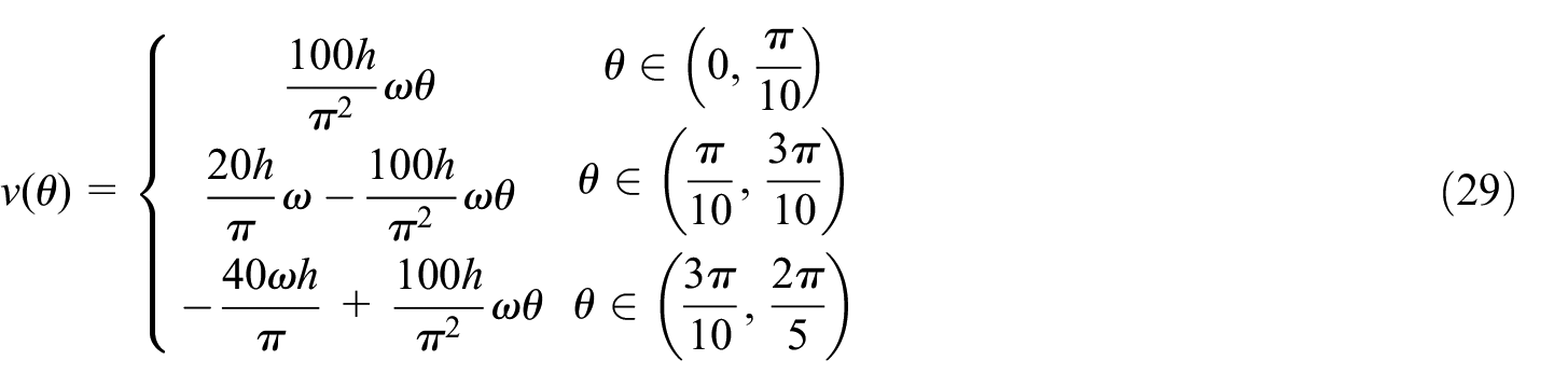
Integrating formula (29) to get the displacement expression of the guide rail assembly in one cycle, which can be written as

$$\begin{array}{c}\multicolumn{1}{c}{s(\theta )=\{\begin{array}{c}\frac{50h}{{\pi }^2}{\theta }^2\hfill \\ \multicolumn{1}{c}{-h+\frac{20h\theta }{\pi }-\frac{50h{\theta }^2}{{\pi }^2}}\\ \multicolumn{1}{c}{7h-\frac{40h\theta }{\pi }+\frac{50h{\theta }^2}{{\pi }^2}}\end{array}\begin{array}{c}\theta \in (0,\frac{\pi }{10})\hfill \\ \multicolumn{1}{c}{\theta \in (\frac{\pi }{10},\frac{3\pi }{10})}\\ \multicolumn{1}{c}{\theta \in (\frac{3\pi }{10},\frac{2\pi }{5})}\end{array}}\end{array}$$

(30)

The contact surface of the guide rail assembly in the oil is a constant acceleration and deceleration surface. The coordinates of the contact point on the curved surface of the 2D piston pump’s guide rail can be expressed as

$$\begin{array}{c}\multicolumn{1}{c}{R_n=\left[\begin{array}{c}{x}_n\hfill \\ \multicolumn{1}{c}{y_n}\\ \multicolumn{1}{c}{z_n}\end{array}\right]=\left[\begin{array}{c}{R}_{\mathrm{p}}·\cos (\theta +\beta )\hfill \\ \multicolumn{1}{c}{-R_{\mathrm{p}}·\sin (\theta +\beta )}\\ \multicolumn{1}{c}{\frac{R_{\mathrm{B}}\omega }{{\omega }_{\mathrm{S}}}+S(\theta )-R_{\mathrm{p}}·\cos \beta \cot \frac{\phi }{2}\cos \alpha }\end{array}\right]}\end{array}$$

(31)

Figure 6 shows the coordinates of the surface of the guide rail, where R_p is the vertical length from the contact point on the curved surface to the central axis of the guide rail. θ is the rotational angle of the guide rail, φ is the vertex angle of the conical track, r_B is the length of the contact point on the outer contour of the guide rail, and R_B is the radius from the contact point on the outer contour of the guide rail to the rotational axis of the guide rail. r_A is the length of the contact point on the outer contour of the guide rail, R_A is the radius from the contact point on the outer contour of the guide rail to the rotational axis of the guide rail, α is the pressure angle, and β is the difference between the contact line angle of the guide rail and θ.

Figure 6.

The coordinates of the surface of the guide rail.

Here β and pressure angle α can be expressed by formulas (32) and (33), respectively:

$$\beta =\arcsin \left\{\cot \frac{\phi }{2}\sin \left[\arctan \frac{v(\theta )}{R_{\mathrm{p}}}\right]\right\}$$

(32)

$$\tan \alpha =\frac{1}{R_{\mathrm{p}}}v(\theta )$$

(33)

Since the linear velocity of the guide rail and the tapered roller at the contact point is the same, it can be obtained as

$$R_{\mathrm{B}}\omega =r_{\mathrm{B}}{\omega }_{\mathrm{S}}$$

(34)

where ω is the angular velocity of the guide rail, and ω_S is the angular velocity of the self-rotation of the stacked cone rollers.

According to formula (31), the outer and inner contour lines of the large guide rail can be expressed by formulas (35) and (36), respectively:

$$\begin{array}{c}\multicolumn{1}{c}{R_{{\mathrm{big}-\mathrm{out}}^{\theta }}=\left[\begin{array}{c}{x}_{{\mathrm{big}-\mathrm{out}}^{\theta }}\hfill \\ \multicolumn{1}{c}{y_{{\mathrm{big}-\mathrm{out}}^{\theta }}}\\ \multicolumn{1}{c}{z_{{\mathrm{big}-\mathrm{out}}^{\theta }}}\end{array}\right]}\\ =\left[\begin{array}{c}{R}_{B\mathrm{big}}·\cos (\theta +\beta )\hfill \\ \multicolumn{1}{c}{-R_{B\mathrm{big}}·\sin (\theta +\beta )}\\ \multicolumn{1}{c}{\frac{R_{B\mathrm{big}}\omega }{{\omega }_S}+S(\theta )-R_{B\mathrm{big}}·\cos \beta \cot \frac{\phi }{2}\cos \alpha }\end{array}\right]\hfill \end{array}$$

(35)

$$\begin{array}{c}\multicolumn{1}{c}{R_{{\mathrm{big}-\mathrm{in}}^{\theta }}=\left[\begin{array}{c}{x}_{{\mathrm{big}-\mathrm{in}}^{\theta }}\hfill \\ \multicolumn{1}{c}{y_{{\mathrm{big}-\mathrm{in}}^{\theta }}}\\ \multicolumn{1}{c}{z_{{\mathrm{big}-\mathrm{in}}^{\theta }}}\end{array}\right]}\\ =\left[\begin{array}{c}{R}_{A\mathrm{big}}\cos (\theta +\beta )\hfill \\ \multicolumn{1}{c}{-R_{A\mathrm{big}}·\sin (\theta +\beta )}\\ \multicolumn{1}{c}{\frac{R_{B\mathrm{big}}\omega }{{\omega }_S}+S(\theta )-R_{A\mathrm{big}}·\cos \beta \cot \frac{\phi }{2}\cos \alpha }\end{array}\right]\hfill \end{array}$$

(36)

where, the R_Bbig of the large guide rail is 25.5 mm, and the R_Abig is 21 mm.

The outer contour line and inner contour line of the small guide rail can be expressed by formulas (37) and (38), respectively.

$$\begin{array}{c}\multicolumn{1}{c}{R_{{\mathrm{small}-\mathrm{out}}^{\theta }}=\left[\begin{array}{c}{x}_{{\mathrm{small}-\mathrm{out}}^{\theta }}\hfill \\ \multicolumn{1}{c}{y_{{\mathrm{small}-\mathrm{out}}^{\theta }}}\\ \multicolumn{1}{c}{z_{{\mathrm{small}-\mathrm{out}}^{\theta }}}\end{array}\right]}\\ =\left[\begin{array}{c}{R}_{B\mathrm{small}}·\cos (\theta +\beta )\hfill \\ \multicolumn{1}{c}{-R_{B\mathrm{small}}·\sin (\theta +\beta )}\\ \multicolumn{1}{c}{\frac{R_{B\mathrm{small}}\omega }{{\omega }_S}+S(\theta )-R_{B\mathrm{small}}·\cos \beta \cot \frac{\phi }{2}\cos \alpha }\end{array}\right]\hfill \end{array}$$

(37)

$$\begin{array}{c}\multicolumn{1}{c}{R_{\mathrm{small}-\mathrm{in}}\theta =\left[\begin{array}{c}{x}_{\mathrm{small}-\mathrm{in}}\theta \hfill \\ \multicolumn{1}{c}{y_{\mathrm{small}-\mathrm{in}}\theta }\\ \multicolumn{1}{c}{z_{\mathrm{small}-\mathrm{in}}\theta }\end{array}\right]}\\ =\left[\begin{array}{c}{R}_{A\mathrm{small}}·\cos (\theta +\beta )\hfill \\ \multicolumn{1}{c}{-R_{\mathrm{Asmall}}·\sin (\theta +\beta )}\\ \multicolumn{1}{c}{\frac{R_{A\mathrm{small}}\omega }{{\omega }_S}+S(\theta )-R_{A\mathrm{small}}·\cos \beta \cot \frac{\phi }{2}\cos \alpha }\end{array}\right]\hfill \end{array}$$

(38)

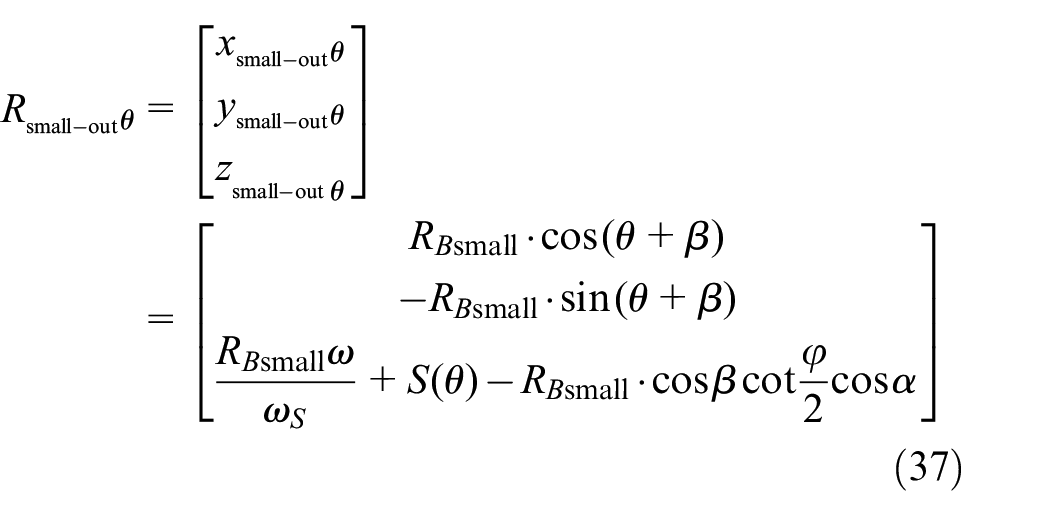
where, the R_Bsmall of the small guide rail is 19.125 mm, and the R_Asmall is 12.75 mm.

Modeling of peripheral churning torque

To clearly model the peripheral churning torque, the contact surface between the cam guide and the oil is divided into five zones, which are represented by different colors, as shown in Figure 7. The zone I is shown in blue, the zone II is shown in red, and the zone III is the cam surface of the large rail, shown in orange. The zone IV is shown in gray, and the zone V is the cam surface of the small rail, shown in green.

Figure 7.

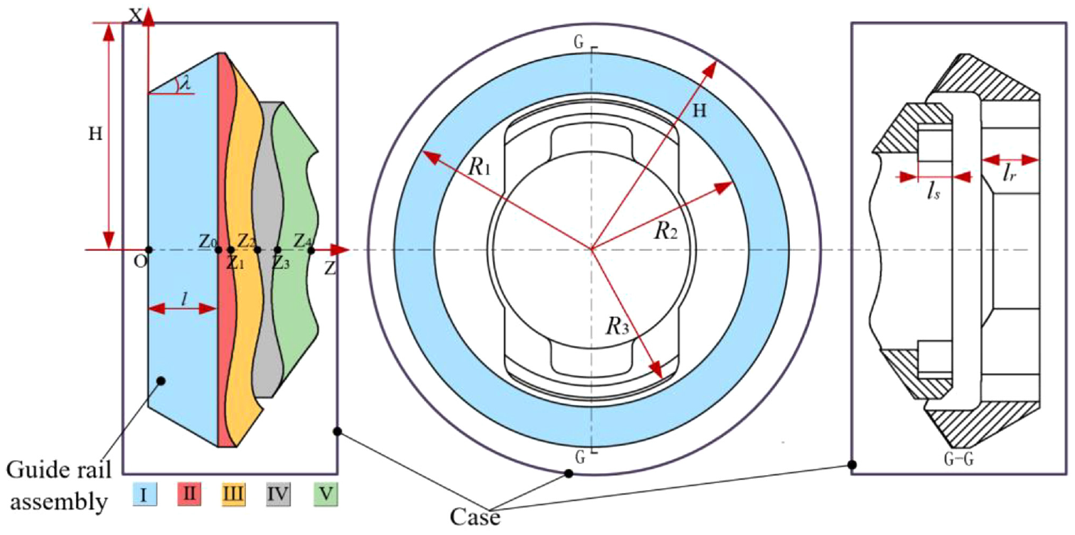
Schematic of contact surface related to peripheral churning torque.

According to Newton’s law of internal friction, the viscous friction force can be expressed as

$$F_v=\mu ·A_{\mathrm{i}}·\frac{\mathrm{du}}{\mathrm{dx}}$$

(39)

where μ is dynamic viscosity of the oil; A_i represents the contact area between the five parts of the above-mentioned cam guide and the oil, i = 1–5; du/dx is the velocity gradient.

Therefore, the viscous internal frictional force and frictional torque of zone I can be expressed as

$$F_{v1}={\int }_0^{Z_0}\mu \frac{\omega (R_2+z\tan \lambda )}{H-R_2-z\tan \lambda }·2\pi zdz$$

(40)

$$M_1={\int }_0^{Z_0}\mu \frac{\omega (R_2+z\tan \lambda )}{H-R_2-z\tan \lambda }·2\pi z·\left(R_2+z\tan \lambda \right)dz$$

(41)

The viscous internal frictional force and frictional torque of zone II can be expressed as

$$F_{v2}={\int }_0^{2\pi }\mu [R_{\mathrm{big}-\mathrm{out}}\left(\theta \right)-z_0]·\frac{\omega R_1}{H-R_1}d\theta$$

(42)

$$\begin{array}{c}{M}_2={\int }_0^{2\pi }\mu [R_{\mathrm{big}-\mathrm{out}}\left(\theta \right)-z_0]·d\theta ·\frac{\omega R_1}{H-R_1}·R_1\hfill \\ R_{\mathrm{big}-\mathrm{out}}(\theta )=\frac{R_{B\mathrm{big}}\omega }{{\omega }_S}+S(\theta )-R_{B\mathrm{big}}·\cos \beta \cot \frac{\phi }{2}\cos \alpha \hfill \end{array}$$

(43)

The viscous internal frictional force and frictional torque of zone III can be expressed as

$$F_{v3}={\int }_0^{2\pi }{\int }_{z_{\mathrm{big}-\mathrm{out}}}^{z_{\mathrm{big}-\mathrm{in}}}\mu ·\frac{\omega x_{\mathrm{big}}\left(\theta \right)}{H-x_{\mathrm{big}}\left(\theta \right)}\mathrm{dz}·x_{\mathrm{big}}\left(\theta \right)d\theta$$

(44)

$$M_3={\int }_0^{2\pi }{\int }_{z_{\mathrm{big}-\mathrm{out}}}^{z_{\mathrm{big}-\mathrm{in}}}\mu ·\frac{\omega x_{\mathrm{big}}\left(\theta \right)}{H-x_{\mathrm{big}}\left(\theta \right)}dz·{x_{\mathrm{big}}}^2\left(\theta \right)d\theta$$

(45)

$$\begin{array}{c}{z}_{\mathrm{big}-\mathrm{in}}=\frac{R_{B\mathrm{big}}\omega }{{\omega }_S}+S(\theta )-R_{A\mathrm{big}}·\cos \beta \cot \frac{\phi }{2}\cos \alpha \hfill \\ z_{\mathrm{big}-\mathrm{out}}=\frac{R_{B\mathrm{big}}\omega }{{\omega }_S}+S(\theta )-R_{B\mathrm{big}}·\cos \beta \cot \frac{\phi }{2}\cos \alpha \hfill \\ x\left(\theta \right)=R_p·\cos (\theta +\beta )\hfill \end{array}$$

(46)

The viscous internal frictional force and frictional torque of zone IV can be expressed as

$$F_{v4}={\int }_0^{2\pi }\mu [Z_{\mathrm{big}-\mathrm{in}}\left(\theta \right)-Z_{\mathrm{small}-\mathrm{out}}\left(\theta \right)]·\frac{\omega R_3}{H-R_3}d\theta$$

(47)

$$\begin{array}{c}{M}_4={\int }_0^{2\pi }\mu [Z_{\mathrm{big}-\mathrm{in}}\left(\theta \right)-Z_{\mathrm{small}-\mathrm{out}}\left(\theta \right)]·\frac{\omega R_3}{H-R_3}d\theta ·R_3\hfill \end{array}$$

(48)

The viscous internal frictional force and frictional torque of zone V can be expressed as

$$F_{v5}={\int }_0^{2\pi }{\int }_{z_{\mathrm{small}-\mathrm{out}}}^{z_{\mathrm{small}-\mathrm{in}}}\frac{\omega x_{\mathrm{small}}\left(\theta \right)}{H-x_{\mathrm{small}}\left(\theta \right)}\mathrm{dz}·x_{\mathrm{small}}\left(\theta \right)d\theta$$

(49)

$$M_5={\int }_0^{2\pi }{\int }_{z_{\mathrm{small}-\mathrm{out}}}^{z_{\mathrm{small}-\mathrm{in}}}\frac{\omega x_{\mathrm{small}}\left(\theta \right)}{H-x_{\mathrm{small}}\left(\theta \right)}\mathrm{dz}·{x_{\mathrm{small}}}^2\left(\theta \right)d\theta$$

(50)

Therefore, the peripheral churning torque generated by the left rail assembly can be obtained as

$$M_{\mathrm{P}}=C_{\mathrm{P}}·(M_1+M_2+M_3+M_4+M_5)$$

(51)

where C_P is a correction coefficient that can be obtained by CFD simulation. This is mainly because Newton’s law of internal friction is only appropriate for the laminar flow state. Considering the influence of surrounding flow field, the peripheral churning process cannot be assumed as ideal laminar flow. Therefore, it needs to add C_P to the peripheral churning torque calculation.

Pushing flow churning torque

In this section, the pushing flow churning torque is analytically modeled. Figure 8 illustrates schematic for pushing flow churning torque of big and small guide rails. Figure 9 shows the main geometric parameter of big and small guide rails.

Figure 8.

Schematic for pushing flow churning torque of big and small guide rails.

Figure 9.

Main geometric parameter of big and small guide rails.

According to the work-energy theorem, the pushing flow resistance force generated by the guide rail assembly accelerating from stationary state to a velocity v can be expressed as

$$d{F}_{\mathrm{p}}\mathrm{dl}=\frac{1}{2}·\rho \mathrm{dSdl}·v^2$$

(52)

where F_p is the pushing flow resistance force; d_S is a micro element area of the contact surface that is pushed; dl is the rotational displacement corresponding to the rotational path element; ρ is the oil density.

The pushing flow churning torque of the large guide rail can be expressed as

$$M_{\mathrm{D}1}=\int \frac{1}{2}·\rho v^2{R}_{\mathrm{s}}\mathrm{ds}=\frac{1}{2}·\rho {\left(\frac{2\pi n}{60}\right)}^2\int {R_{\mathrm{s}}}^3\mathrm{ds}$$

(53)

where R_s is the distance from the piezoresistive point to the origin of the radius.

In the Cartesian coordinate system, the function of radius R_s is treated as a piecewise function. Considering dS = l_r d_y, it can be obtained

$$\begin{array}{c}{M}_{\mathrm{D}1}=C_{\mathrm{D}}\frac{{\pi }^2}{1800}·\rho n^2{l}_{\mathrm{r}}·\hfill \\ (\int \begin{array}{c}{y}_3\hfill \\ \multicolumn{1}{c}{y_1}\end{array}{\sqrt{{c_{\mathrm{r}}}^2+y^2}}^3\mathrm{dy}+\int \begin{array}{c}{y}_7\hfill \\ \multicolumn{1}{c}{y_3}\end{array}{\sqrt{y^2+f1{(y)}^2}}^3\mathrm{dy}+\int \begin{array}{c}{y}_8\hfill \\ \multicolumn{1}{c}{y_7}\end{array}{\sqrt{y^2+f2{(y)}^2}}^3\mathrm{dy})\hfill \end{array}$$

(54)

where f1(y) is the function that describes the curve from point l_B to l_C; f2(y) is the function that describes the curve from point l_C to l_D; y₁, y₃, y₇, y₈ are the coordinates corresponding to l_A, l_B, l_C, l_D, respectively; c_r is the abscissa corresponding to l_A; C_D is the correction coefficient of pushing flow churning torque, which can be obtained by CFD simulation.

Similarly, the pushing flow churning torque of the small guide rail can be obtained as

$$\begin{array}{c}{M}_{\mathrm{D}2}=C_{\mathrm{D}}\frac{{\pi }^2}{1800}·\rho n^2{l}_{\mathrm{s}}·\hfill \\ (\int \begin{array}{c}{y}_3\hfill \\ \multicolumn{1}{c}{y_2}\end{array}{\sqrt{{c_{\mathrm{s}}}^2+y^2}}^3\mathrm{dy}+\int \begin{array}{c}{y}_4\hfill \\ \multicolumn{1}{c}{y_3}\end{array}{\sqrt{y^2+f3{(y)}^2}}^3\mathrm{dy}+\int \begin{array}{c}{y}_5\hfill \\ \multicolumn{1}{c}{y_4}\end{array}{\sqrt{y^2+f4{(y)}^2}}^3\mathrm{dy})\hfill \end{array}$$

(55)

where f3(y) is the function that describes the curve from point l_F to l_G; f4(y) is the function that describes the curve from point l_G to l_H; y₂, y₄, y₅, y₆ are the coordinates corresponding to l_E, l_F, l_G, l_H, respectively; c_S is the abscissa corresponding to l_E.

Therefore, the pushing flow churning torque of the left guide rail assembly is

$$M_{\mathrm{D}}=M_{\mathrm{D}1}+M_{\mathrm{D}2}$$

(56)

Combining three formulas (26), (51), and (56), the total churning torque can be finally written as

$$M_{\mathrm{T}}=M_{\mathrm{E}}+M_{\mathrm{P}}+M_{\mathrm{D}}$$

(57)

The above analytical modeling process clearly reveals that the total churning torque consists of three subcomponents: the peripheral churning torque, the pushing flow churning torque, and the end face churning torque. Formula (57) will be used to calculate both the total churning torque and three subcomponents, which will be compared and verified by the CFD simulation results.

CFD numerical simulation

In this section, the CFD techniques is used to simulate the churning torque of the guide rail assembly in order to verify the accuracy of the analytical model in Section “Analytical modeling,” and also obtain the three correction coefficients in formulas (16), (51), and (54). First of all, it is necessary to determine the shape and size of the fluid domain where the churning loss of the guide rail assembly occurs. Figure 10 shows the fluid domain includes walls, churning parts, and fluid zones, and its geometric dimensions are exactly the same as the actual ones. The detailed parameters are listed in Table 1. It is known that the axial reciprocating motion of the cam guide rail has little effect on its churning torque, ¹⁹ therefore the simulation would total focus on rotational churning behavior. The rotational speed during simulation is controlled by programming UDFs with different speeds in Fluent software. In addition, the dynamic grid method is used to simulate the dynamic behavior of flow field and the RNG k-ε model is used to consider the effect of turbulent flow. The data of the churning parts rotational 360° is recorded as the simulation result.

Figure 10.

Schematic diagram of the fluid domain of the guide rail assembly.

Table 1.

Detailed parameters of fluid domain.

Parameter	Value
The diameter of the fluid domain Lz	57 mm
The width of the fluid domain	27 mm
Overall thickness of guide rail assembly Hb	22 mm
Thickness of large guide rail Hb1	15 mm
Thickness of small guide rail Hb2	10.75 mm
Diameter of large guide rail D1	51 mm
Diameter of small guide rail D2	37.5 mm
Groove radius for large guide rail Rb1	19.5 mm
Groove radius for large guide rail Rb2	13.5 mm
Groove radius for small guide rail Rs3	16.5 mm
Groove radius for small guide rail Rs4	12.75 mm
Groove thickness of large guide rail lr	7.5 mm
Groove thickness of small guide rail ls	4.5 mm
Oil temperature	40°C
Oil density	850 kg/m3
Oil dynamic viscosity	0.03979 Pa s
Speed range of rotation	1000–16,000 rpm

The grid number has a crucial influence on the accuracy of the CFD simulation results. Meanwhile, too many grid numbers would over-consume computing resources. In this paper, five different grid numbers are picked for the CFD simulation, which are 0.2, 0.4, 0.7, 1.04, and 1.35 million, respectively. The average churning torques with these different grid numbers are simulated with a rotational speed of 16,000 rpm, as shown in Figure 11. It can be seen that the churning torques fluctuate from 0.74 to 0.83 N m with these five increasing grid numbers, which indicates that increasing the grid number could improve simulation accuracy since it would capture more detailed features of flow field. However, when the grid numbers increase from 1.04 to 1.35 million, the churning torque remains almost unchanged. Therefore, 1.04 million grid number was finally selected as a compromise between computing resources and simulation accuracy.

Figure 11.

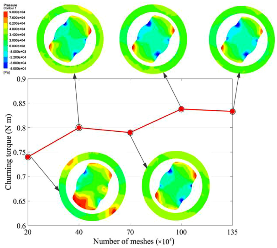
Average torque and pressure distribution of different grid numbers.

The CFD simulation is performed based on the above settings. Figure 12 illustrates the instantaneous torque with rotational speeds of 1000 and 16,000 rpm, and grid number of 1.04 and 1.35 million. It can be found that the churning torque increases with increasing the rotational speed, and it almost stays stable with varying the rotational angle. Besides, the whole instantaneous torques also remain unchangeable with grid number of 1.04 and 1.35 million, thus again verify the correctness of above-mentioned grid number selection.

Figure 12.

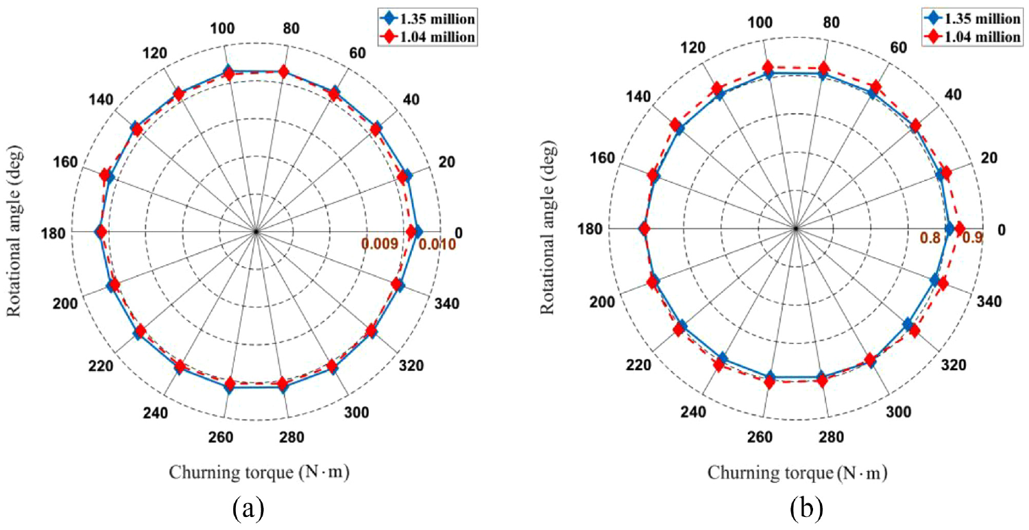
Instantaneous torque obtained by CFD: (a) 1000 rpm and (b) 16,000 rpm.

Figure 13 shows the variation of the three subcomponents of churning torque calculated by CFD in the range of 0°–30° when the rotational speed is 16,000 rpm. It can be seen that the end face churning torque and the peripheral churning torque basically change linearly, while the pushing flow churning torque varies in an approximate triangular wave, which may be due to the U-shaped groove structure of the large and small guide rails that causes the pushing flow torque to fluctuate with the angle. After averaging the torques of each subcomponent, the CFD simulated results can be used to verify the analytical modeling results. Figure 14 illustrates the comparison of analytical and simulated results of churning torque with different rotational speeds. It should be noted that in this paper the analytical calculation takes the correction coefficients of C_E, C_P, and C_D as 1.05, 43.99, and 0.051. The rising trend of the analytical and the simulated results are basically the same. With the increase of the pump speed, the total churning torque presents a monotonic increasing trend, whose slope gradually increases. It shows that the higher the rotational speed, the faster the total churning torque increases. At 16,000 rpm, the analytical value and simulation value are 0.826 and 0.838 N m, respectively. This indicates the analytical value is in good agreement with the simulated counterpart.

Figure 13.

Churning torque of three subcomponents at 16,000 rpm.

Figure 14.

Churning torque comparison between analytical and CFD simulation results.

Besides, the three subcomponents of churning torque also increase with the increase of rotational speed. Here, takes the analytical value as an example. At the rotational speed of 16,000 rpm, the end face churning torque is about 0.060 N m, accounting for 7.3% of the total torque. The peripheral churning torque is about 0.458 N m, accounting for 55.4% of the total torque. The pushing flow churning torque is about 0.308 N m, accounting for 37.3% of the total torque. Among them, the end face and peripheral churning torque are both viscous frictional force, which basically changes linearly in the whole speed range. While the pushing flow churning torque gradually warps with the increase of the speed. In this point, the CFD simulation results are consistent with the analytical counterparts.

The above analysis has a good guiding significance for the reduction optimization of churning torque. Firstly, the structural features of the cam guide assembly determine that the viscous frictional force plays a leading role in total churning loss, where the end face and the peripheral churning torque accounts for about 62.7% of the total torque. However, the pushing flow churning torque increases rapidly, indicating that with the increase of the rotational speed, the influence of the inertial force on the flow field becomes much more significant. Secondly, among the three subcomponents of churning torque, the proportion of the peripheral churning torque is the largest, the pushing flow torque is the second, and the end face torque is the lowest. Generally speaking, the peripheral churning torque seems to be the top choice for structural parameter optimization. However, according to the previous formulas (40)–(51), the peripheral churning torque is mainly related to the radius R₁ and R₂ of the large and small guide rails and the height Z₀, Z₁, Z₂, Z₃, and Z₄ of the end faces of each part, where these parameters are closely related to the main working performance of the pump. Once the pump specifications and performance parameters are determined, there is little room for these parameters to change. Therefore, the optimization of structural parameters should focus on the pushing flow churning torque. Figure 15 shows the structural parameters related to the pushing flow churning torque. It can be seen that the pushing flow churning torque mainly comes from the large U-shaped groove and the small U-shaped groove on the large and small guide rails. And the function of these two U-shaped grooves is only used to fix the bayonet shaft. Thus, if the structural strength allows, the pushing flow churning torque can be effectively reduced by reducing the outer diameter of the assembly of bayonet shaft-transmission shaft, namely, reducing the length of the bottom edges of the oil pushing surfaces S₁ and S₂, l₁ and l₂. Similarly, reducing the depth of the two U-shaped grooves, l_s and l_r, can also achieve the same effect.

Figure 15.

Schematic diagram of structural parameters related to pushing flow churning torque.

Figures 16 and 17 show the velocity vector distribution diagram and pressure distribution diagram of cross-section of the cam guide rail assembly fluid domain obtained by CFD simulation when the guide rail rotates at 1000, 7000, 10,000, and 15,000 rpm, respectively. The former can be used to explain the cause of viscous churning torque, and the latter can be used to explain the mechanism of pushing flow churning torque. It can be seen that in the peripheral annular gap in Figure 16, the flow velocity of the fluid in contact with the guide rail is the highest, and the velocity gradually decreases outward along the radial direction until the edge of the fluid domain is close to zero. This velocity distribution conforms to Newton’s law of internal friction, revealing that the churning torque in the annular gap is viscous frictional force, which is consistent with the previous analytical modeling. Similarly, for the fluid region in the central region, the flow velocity of the fluid contacting with the guide rail is the highest, and then decreases in turn. Since the fluid in the central region is far away from the guide rail, it almost does not participate in the oil churning behavior, whose velocity is basically zero. With the increase of pump speed, the flow speed of fluid is also increasing, and the corresponding viscous churning torque is also increasing.

Figure 16.

Velocity vector distribution of flow field at different rotational speeds: (a) 1000 rpm, (b) 7000 rpm, (c) 10,000 rpm, and (d) 15,000 rpm.

Figure 17.

Pressure distribution of flow field at different rotational speeds: (a) 1000 rpm, (b) 7000 rpm, (c) 10,000 rpm, and (d) 15,000 rpm.

In addition to the viscous frictional force, there also exists pushing flow resistance force for the fluid in the central region. The mechanism can be revealed by analyzing the pressure distribution diagram. It can be seen from Figure 16 that for the peripheral annular gap, the pressure at the edge of the fluid domain is the highest, and the pressure near the guide rail is the lowest. The pressure gradually decreases along the radial direction, which is consistent both with Bernoulli’s law and the result of velocity vector distribution analysis in Figure 16. For the fluid in the central region, due to the counterclockwise rotation of the guide rail, a high-pressure zone and a low-pressure zone of the U-shaped groove can be clearly found. The formation of the high-pressure zone is due to the oil pushed by the U-shaped groove, which causes the oil to lean toward the contact surface of the guide rail and thus leads to the pressure rise. While for the low pressure zone the situation is the opposite. It is due to the pressure drop caused by the oil being churned and accelerated away from the contact surface of the guide rail. It is the existence of high- and low-pressure areas on both sides of the U-shaped groove that the pushing flow churning torque is generated. With the increase of the pump speed, the pressure in the high-pressure zone becomes higher, while the pressure in the low-pressure zone becomes lower, which reveals that the pushing flow churning torque will rise rapidly with the increase of the pump speed.

Experiments and discussions

In order to verify the accuracy of the analytical modeling and CFD simulation, a churning torque test platform is specially designed and built, as shown in Figure 18. The platform is mainly composed of a driving motor and regulator, a SL06 torque/speed sensor, and a churning prototype. The driving motor and regulator is used to drive the churning prototype and adjust its rotational speeds. The torque/speed sensor is used to measure the churning torque and rotational speed of churning prototype. Figure 19 shows the pictures of churning prototype that wholly immersed in the tested cavity.

Figure 18.

Test platform for the churning torque.

Figure 19.

Pictures of churning prototype.

During the experiment the tested guide rail is fixedly connected with the tested shaft, and the tested shaft drives it to rotate synchronously. However, the rotation of the tested shaft also creates resistance, and in addition, the entire drive chain also has resistance during rotation. Therefore, before the formal experiment, the resistance torque generated by both the tested shaft and drive chain needs to be measured as the background. The net churning torque produced by the guide rail is the difference between the measured total torque and the background torque.

In order to prove the repeatability of the experiment, the churning torque was repeatedly measured three times at both 5000 and 10,000 rpm respectively, as shown in Figure 20. At 5000 rpm, the measured churning torque fluctuates in the range of 0.134−0.147 N m. At 10,000 rpm, the measured churning torque fluctuates in the range of 0.361−0.382 N m. It can be seen that the fluctuation of the two groups of data is relatively small, which proves the repeatability of the experiment.

Figure 20.

Experiment repeatability at two different rotational speeds: (a) 5000 rpm and (b) 10,000 rpm.

Figure 21 shows the comparison of analytical, CFD, and experimental results. It is found that the three curves are in good agreement, all of which are monotonically increasing curves with the increase of rotational speed. When the speed reaches 16,000 rpm, the analytical, CFD, and experimental results are about 0.83, 0.82, and 0.78 N m respectively, with the maximum error of about 6%. Therefore, the experimental results verify the correctness of both analytical modeling and CFD simulation. There is a certain deviation between the experimental results of oil churning loss and the simulation results, and this deviation mainly comes from two sources. First of all, in the CFD numerical simulation, the viscosity and density of the oil are directly given without considering the viscosity-temperature characteristics of the oil. However, in the actual experiment process, the temperature change of the oil will lead to the viscosity change, which makes the experimental results deviate from the CFD numerical simulation results. Subsequently, this conjecture was verified in the analytical model. Another reason is that there may be certain errors in the processing and installation of the test rotor, resulting in deviations in the coaxiality at high speeds, resulting in a slight difference between the experimental results and the simulation results.

Figure 21.

Comparison of analytical, CFD, and experimental results of churning torque.

Table 2 shows the comparison of the initial torque and oil churning torque at different speeds of the stacked rollers 2D piston pump, and the table displays the proportion of the oil churning torque at different speeds. It can be seen that as the speed increases, the proportion of churning torque gradually increases, and the influence on the initial torque gradually intensifies, which further proves the necessity of this research.

Table 2.

Comparison between the initial torque value of the pump and the churning loss torque.

Parameter	Value
Rotating speed (rpm)	1000	2000	3000	4000	5000	6000	7000	8000	9000	10,000
Churning torque (N m)	0.06	0.08	0.11	0.12	0.14	0.20	0.25	0.29	0.32	0.37
Initial torque (N m)	0.9	1.02	1.25	1.36	1.55	1.85	2.15	2.45	2.7	2.9
Impact percentage (%)	6.67	7.84	8.8	8.97	9.03	10.81	11.63	11.84	11.85	12.76

Due to the mechanism of frictional heat generation, when the guide rail assembly is churned in the oil, the oil temperature will increase and the viscosity will decrease. Such thermal effects also directly influence the churning torque. In previous studies, dynamic viscosity is usually considered as constant. ³¹ This paper also researches the change of oil viscosity in churning loss when the experimental speed is increased from 0 to 16,000 rpm. Firstly, the rotational speed is raised to the target value in about 5 s, and then this target speed is maintained for 10 s. A temperature sensor is used to record the temperature which should be maintained for 10 s, and then continue to increase until it reaches 16,000 rpm. The experimental results are shown in Figure 22(a). The oil temperature curve shows that when the speed exceeds 4000 rpm, the oil temperature begins to rise. And as the speed increases, the overall temperature rises faster. It is known that the viscosity-temperature characteristics of 46# hydraulic oil can be represented by formula (58), which is ³²

$$\mu =0.188e^{-0.0471T}$$

(58)

Figure 22.

Influence of oil viscosity on churning torque: (a) oil temperature rise curve and (b) consider the viscosity-temperature characteristics.

Substituting formula (58) into formula (57), the churning torque of the guide rail considering the viscosity-temperature characteristics can be obtained, as shown in Figure 22(b). The yellow curve shows that the churning torque with viscosity-temperature characteristics being considered, while the red one does not. The yellow curve is more consistent with the experimental result. The reason is that the dynamic viscosity of the oil decreases with the increase of temperature, while the peripheral churning torque and the end face churning torque are both proportional to the viscosity. This proves that the accuracy of the analytical model can be further improved by considering the viscosity-temperature characteristics.

Conclusion

• (1) To conveniently calculate the churning torque and also provide guidance for future optimization of churning torque reduction, an analytical model of constant acceleration and constant deceleration cam guide rail assembly of the stacked-rollers 2D piston pump is established. With the increase of pump speed, the churning torque presents a monotonic increasing trend, which reaches about 0.826 N m at 16,000 rpm of pump rotational speed. The analytical results agree well with both CFD simulation and experimental results, thus verifying the modeling accuracy.

• (2) Analytical modeling clearly reveals that the total churning torque consists of three subcomponents: peripheral churning torque, the pushing flow churning torque, and the end face churning torque. When the pump speed is 16,000 rpm, these three sub-components account for 7.3%, 55.4%, and 37.3% of the total churning torque respectively. Thus laying a good theoretical foundation for the follow-up study on the optimization of structural parameters to reduce the oil churning torque.

• (3) Since the structural parameters related to the peripheral churning torque have little margin for adjust. The future optimization should focus on the pushing flow churning torque. This can be effectively reduced by reducing the outer diameter of assembly of bayonet shaft and transmission shaft, namely, reducing the length of the bottom edges of the oil pushing surfaces of two U-grooves. Similarly, reducing the depth of the two U-grooves can achieve the same effect.

• (4) The accuracy of the analytical model can be further improved by considering the viscosity-temperature characteristics.