Sage Journals: Discover world-class research

Abstract

As a result of the ongoing upgrading of the manufacturing industries, higher and higher requirements are being proposed for assembly precision. In particular, in the industries that involve assembly of large-sized products, it is hoped that assembly accuracy can still be guaranteed as the product size increases. The emergence of the indoor Global Positioning System (iGPS) will enable this demand to be met. In this work, we have conducted in-depth research on the measurement principles and the dynamic measurement performance of the iGPS measurement system. In addition, based on the motion equation for the tracked target, an analytical method to calculate the compensation amount required for dynamic measurements is proposed. This method is suitable for accurate measurement of the actual trajectory of a target in real time when the theoretical trajectory of this tracked target is known. We set up a simulation environment in MATLAB and tested the proposed method. The simulation testing proved that the method can compensate effectively for errors in iGPS dynamic measurement.

Keywords

iGPS dynamic tracking mathematical model error compensation MATLAB simulation trajectory measurement

Introduction

As the various industrial needs of humanity (e.g., space exploration, national defense, energy exploration) continue to increase, it has become increasingly necessary to manufacture large-scale industrial equipment, including rockets, aircraft, and submarines.^1,2 To improve assembly accuracy during the process of assembling this large-scale industrial equipment, it is necessary to use workshop measurement equipment to measure and locate important positions and to track and measure dynamic work units, such as automated guided vehicles (AGVs) and industrial robots.^3–5

Among the many measurement devices in current use, laser trackers and the indoor Global Positioning System (iGPS) are in particularly wide use in workshops. Of these devices, the laser tracker offers the advantages of high measurement accuracy and a good dynamic performance, but it still has certain disadvantages, including a relatively small measurement range, high cost, and an inability to track multiple targets simultaneously. The iGPS is a relatively recent surveying instrument that has been used widely in industrial production applications because of advantages that include a large measurement range and a capability for simultaneous measurement of multiple targets.⁶

Over the past two decades, large numbers of researchers have studied the measurement performance of iGPS. However, most of this research has focused on static measurement of the iGPS measurement system.^7–11. In recent years, with the emergence of the concept of digital assembly, the iGPS is being used widely to track dynamic targets to enable completion of high-precision assembly. However, because of the measurement principle of the iGPS, the system does not have very good dynamic characteristics. As a result, some researchers have begun to study the dynamic characteristics of the iGPS.^12,13 Using the programmability of industrial robots, Wang et al. compared the dynamic measurement performances of the iGPS and laser trackers and visualized their results.¹⁴ Depenthal built an experimental environment to study and compare the dynamic measurement characteristics of the iGPS and laser trackers during tracking of targets that move with a circular motion.¹⁵ The studies noted above only summarized their measurement results to a certain extent and did not quantify the relationship between the dynamic characteristics and various measurement factors or perform follow-up research to improve the system’s dynamic characteristics. To improve the measurement accuracy of the iGPS when tracking dynamic targets, Zhao et al. proposed mathematical models of new iGPS single-station and two-station measurement systems that considered the speed of the tracked target and verified corrections of the mathematical models through simulations and physical experiments, but this study only considered the case in which the tracked target moves in a straight line at a uniform speed and thus lacks universal applicability¹⁶. Zeng et al. proposed an algorithm that allowed an AGV to be tracked dynamically when using an iGPS. The algorithm was based on the measurement data obtained from the iGPS to measure the position of the AGV in real time and ensure that the AGV could return adaptively to its established track. The limitation of this algorithm is that the dynamic measurement data from the iGPS are considered to be correct in real time, and thus this algorithm can only be used to perform rough measurement and tracking of the AGV;¹⁷ the approaches proposed by Schmitt et al.¹⁸ and Chen et al.¹⁹ have similar problems.

This paper focuses on a method to improve the dynamic measurement performance of the iGPS when using iGPS measurements to track dynamic targets. When we use a specific measurement instrument to track a moving target dynamically, three trajectories will be produced: the theoretical planning trajectory, the measured trajectory, and the real trajectory. This paper proposes a new dynamic data processing algorithm that is suitable for application to iGPS measurement systems. The dynamic measurement results from these systems are corrected using the theoretical planning trajectory and the iGPS measurement principle to eliminate the dynamic uncertainty caused by the iGPS measurement principle. First, we use the proposed data processing algorithm to correct the measurement-related errors of the iGPS single-station measurement system. Then, we substitute the corrected measurement results from a single-station measurement system into a dual-station measurement system, and subsequently perform secondary corrections to the dual-station measurement system results to obtain the final corrected measurement results. To verify the correctness of the proposed data processing algorithm, we use MATLAB to construct an iGPS measurement environment and then test the proposed algorithm in this environment. From the simulation experiment results, we found that the accuracy of the measurement results was improved significantly after the proposed compensation algorithm was used to correct the measurement data.

Mathematical model

In this section, the principle of the iGPS will be described briefly. The mathematical model of the proposed compensation algorithm will then be described in detail in the subsequent section.

A brief description of the principle of iGPS measurement

Because large numbers of papers have described the iGPS measurement principle in detail, this paper only provides a brief description of this principle. The iGPS is a laser-based indoor optical measurement instrument that is mainly composed of transmitters, receivers, and a position calculation engine (PCE). The iGPS transmitter emits three signals: an infrared light-emitting diode (LED) strobe and two infrared laser-fanned beams. The infrared laser signals rotate in tandem with the transmitter. When the detector receives the LED strobe signal, the time point t₀ is recorded, indicating the time point at which the measurement of the cycle begins, When the receiver receives the two infrared laser fanned beams, it records the time points t₁ and t₂, and then calculates the normal vectors n₁(t₁) and n₂(t₂) for the two infrared laser fanned beams, respectively, when they trigger the receiver according to their recorded time points. From this process, the vector from the receiver to the transmitter can be calculated using equation (1).

n = n_{1} (t_{1}) \times n_{2} (t_{2})

(1)

as shown in Figure 1.

Figure 1.

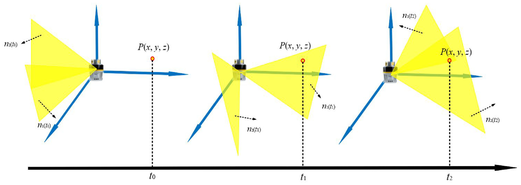
Schematic showing the measurement principle and the measurement process involved when a transmitter measures a detector.

Therefore, it is possible to solve for the horizontal angle (azimuth, φ) and the vertical angle (elevation, θ) when a transmitter is used to measure the receiver. When two transmitters are used to measure the position of a receiver according to its measured azimuth angle and elevation angle in combination with the position of the transmitter in the global coordinate system, then according to the intersection principle, the coordinates of the receiver in the global coordinate system can be calculated as shown in Figure 2.

Figure 2.

Schematics showing the measurement data that are obtained when measuring with one transmitter and illustrating the measurement principle by which coordinates are obtained when measuring with two transmitters.

From the description of the iGPS measurement principle above, we can see that use of a single-station measurement system to complete measurement of the azimuth and elevation requires a time period rather than a time point. When a double-station measurement system is used to complete a target measurement in the global coordinate system, two single-station measurements within a time period are also required. When iGPS is used to measure a static target, this measurement principle will not cause errors in the measurement results, but when the measured target is constantly moving, the target position changes within a measurement period, and this will lead to errors due to the measurement principle. To date, it is believed that when the iGPS is used to perform dynamic measurements, the measurement uncertainties include: systematic uncertainty, random uncertainty, and measurement principle uncertainty (as given by equation (2)).

U_{T} = U_{S} + U_{R} + U_{M}

(2)

Among these uncertainties, U_T represents the total uncertainty, U_S represents the system uncertainty, U_R represents a random uncertainty, and U_M represents the uncertainty caused by the measurement principle. In the next section, the mathematical model of the algorithm proposed in this paper to eliminate the uncertainty due to the measurement principle (U_M) will be described in detail.

Mathematical model of correction algorithm for single station system

This algorithm involves two time axes, where one is the absolute time axis, which starts from the instant when the tracked target begins to move, and the other is the relative time axis, which starts when the sensor receives the strobe signal from the transmitter, as a measurement cycle. In this article, t is used to represent the time point on the relative time axis, and t_(abs) is used to represent the time point on the absolute time axis.

Before we use the iGPS to track the moving target, we already know the theoretical motion trajectory of the moving target and the motion equation along the absolute time axis, as shown in equations (3) and (4).

f_{p} (x, y, z) = 0

(3)

{\begin{matrix} x_{t} = f_{x} (p) \\ y_{t} = f_{y} (p) \\ z_{t} = f_{z} (p) \end{matrix}, p = f_{p} (t_{(abs)})

(4)

Among these parameters, (x_t, y_t, z_t) represent the coordinates of the tracked target, and p represents the motion parameters (e.g., when the tracked target is a tool at the end of a robot, p represents the rotation angle of each axis of the robot; however, when the tracked target is an AGV, p represents the distance moved by the AGV), and p is a function of the movement time t_(abs). At the same time, the motion equation of the first infrared laser-fanned beam emitted by the transmitter can be calculated in the transmitter coordinate system, as shown in equation (5).

\begin{matrix} F_{1} : {\begin{matrix} a_{1} (t) \cdot x + b_{1} (t) \cdot y + c_{1} (t) \cdot z = 0 \\ a_{1 ub} (t) \cdot x + b_{1 ub} (t) \cdot y + c_{1 ub} (t) \cdot z \leq 0 \\ a_{1 lb} (t) \cdot x + b_{1 lb} (t) \cdot y + c_{1 lb} (t) \cdot z \geq 0 \end{matrix} \\ [\begin{matrix} a_{1} (t) \\ b_{1} (t) \\ c_{1} (t) \end{matrix}] = [\begin{matrix} \cos (ω \cdot t) & - \sin (ω \cdot t) & 0 \\ \sin (ω \cdot t) & \cos (ω \cdot t) & 0 \\ 0 & 0 & 1 \end{matrix}] \cdot [\begin{matrix} a_{1} \\ b_{1} \\ c_{1} \end{matrix}] \end{matrix}

(5)

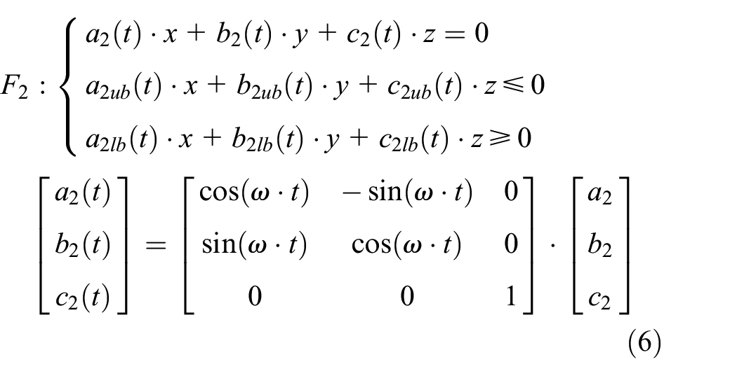
Among these parameters, a₁(t), b₁(t), and c₁(t) constitute the normal vector [a₁(t) b₁(t) c₁(t)]^T of the first infrared laser fanned beam at any time point. [a₁b₁c₁]^T represents the normal vector of the first infrared laser-fanned beam at the beginning of the measurement cycle. Because the infrared laser signal emitted by the transmitter is not a complete spatial plane, but instead represents a radial plane with a specific range of angles, the boundaries must be constrained. Two constraints limit the radiation range of the first infrared laser-fanned beam. Among these constraints, [a_1ub(t) b_1ub(t) c_1ub(t)]^T represents the normal vector of the upper boundary plane of the first infrared laser signal, [a_1lb(t) b_1lb(t) c_1lb(t)]^T represents the normal vector of the lower boundary plane of the first infrared laser signal, and the variation of this vector with time is the same as the variation of the normal vector of the infrared laser signal with time. Similarly, the motion equation for the second fan beam is as shown in equation (6).

\begin{matrix} F_{2} : {\begin{matrix} a_{2} (t) \cdot x + b_{2} (t) \cdot y + c_{2} (t) \cdot z = 0 \\ a_{2 ub} (t) \cdot x + b_{2 ub} (t) \cdot y + c_{2 ub} (t) \cdot z \leq 0 \\ a_{2 lb} (t) \cdot x + b_{2 lb} (t) \cdot y + c_{2 lb} (t) \cdot z \geq 0 \end{matrix} \\ [\begin{matrix} a_{2} (t) \\ b_{2} (t) \\ c_{2} (t) \end{matrix}] = [\begin{matrix} \cos (ω \cdot t) & - \sin (ω \cdot t) & 0 \\ \sin (ω \cdot t) & \cos (ω \cdot t) & 0 \\ 0 & 0 & 1 \end{matrix}] \cdot [\begin{matrix} a_{2} \\ b_{2} \\ c_{2} \end{matrix}] \end{matrix}

(6)

The transmitter and receiver are used to complete a measurement to obtain the measurement results for t₁ and t₂ (t₀=0, on the time axis within a single measurement cycle of the transmitter), and then the equation for the first infrared laser fanned beam at t₁ and the equation for the second infrared laser fanned beam at t₂ are determined according to the measurement results, as shown in equations (7) and (8), respectively.

F_{1} (t_{1}) : {\begin{matrix} a_{1} (t_{1}) \cdot x + b_{1} (t_{1}) \cdot y + c_{1} (t_{1}) \cdot z = 0 \\ a_{1 u b} (t_{1}) \cdot x + b_{1 u b} (t_{1}) \cdot y + c_{1 u b} (t_{1}) \cdot z \leq 0 \\ a_{1 l b} (t_{1}) \cdot x + b_{1 l b} (t_{1}) \cdot y + c_{1 l b} (t_{1}) \cdot z \geq 0 \end{matrix}

(7)

F_{2} (t_{2}) : {\begin{matrix} a_{2} (t_{2}) \cdot x + b_{2} (t_{2}) \cdot y + c_{2} (t_{2}) \cdot z = 0 \\ a_{2 u b} (t_{2}) \cdot x + b_{2 u b} (t_{2}) \cdot y + c_{2 u b} (t_{2}) \cdot z \leq 0 \\ a_{2 l b} (t_{2}) \cdot x + b_{2 l b} (t_{2}) \cdot y + c_{2 l b} (t_{2}) \cdot z \geq 0 \end{matrix}

(8)

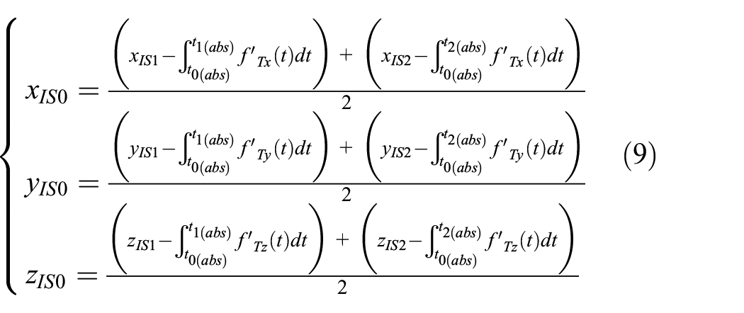
The joint solution to the equations for the determined infrared laser fanned beams and the theoretical trajectory of the moving target can be used to obtain the coordinates (x_IS₁, y_IS₁, z_IS₁) when the moving target meets the first infrared laser fanned beam, and the coordinates (x_IS₂, y_IS₂, z_IS₂) when the moving target meets the second infrared laser fanned beam. Substitution of the encounter coordinates resolved above into the motion equation for the moving target can allow the times t_1(abs), t_2(abs), and t_0(abs) to be obtained when the moving target moves to position (x_IS₁, y_IS₁, z_IS₁) and position (x_IS₂, y_IS₂, z_IS₂) along the absolute time axis. On this basis, the coordinates of the moving target at the time t_0(abs) are calculated as shown in equation (9).

{\begin{matrix} x_{IS 0} = \frac{(x_{IS 1} - \int_{t_{0 (abs)}}^{t_{1 (abs)}} {f'}_{Tx} (t) dt) + (x_{IS 2} - \int_{t_{0 (abs)}}^{t_{2 (abs)}} {f'}_{Tx} (t) dt)}{2} \\ y_{IS 0} = \frac{(y_{IS 1} - \int_{t_{0 (abs)}}^{t_{1 (abs)}} {f'}_{Ty} (t) dt) + (y_{IS 2} - \int_{t_{0 (abs)}}^{t_{2 (abs)}} {f'}_{Ty} (t) dt)}{2} \\ z_{IS 0} = \frac{(z_{IS 1} - \int_{t_{0 (abs)}}^{t_{1 (abs)}} {f'}_{Tz} (t) dt) + (z_{IS 2} - \int_{t_{0 (abs)}}^{t_{2 (abs)}} {f'}_{Tz} (t) dt)}{2} \end{matrix}

(9)

The measurement results (i.e., t₁ and t₂) are corrected according to the coordinates (x_IS₀, y_IS₀, z_IS₀) of the moving target at time t₀, as shown in equation (10).

\begin{matrix} {\begin{matrix} a_{1} (t_{1} + Δ t_{1}) \cdot x_{IS 0} + b_{1} (t_{1} + Δ t_{1}) \cdot y_{IS 0} + c_{1} (t_{1} + Δ t_{1}) \cdot z_{IS 0} = 0 \\ a_{2} (t_{2} + Δ t_{2}) \cdot x_{IS 0} + b_{2} (t_{2} + Δ t_{2}) \cdot y_{IS 0} + c_{2} (t_{2} + Δ t_{2}) \cdot z_{IS 0} = 0 \end{matrix} \\ \to {\begin{matrix} t_{1 (fix)} = t_{1} + Δ t_{1} \\ t_{2 (fix)} = t_{2} + Δ t_{2} \end{matrix} \end{matrix}

(10)

Among these parameters, Δt₁ and Δt₂ represent the corrections to the measurement results t₁ and t₂, respectively. In addition, t_1(fix) and t_2(fix) are the corrected measurement results. The corrected normal vectors n₁(t_1(fix)) and n₂(t_2(fix)), and the receiver-to-transmitter vector are then calculated from the corrected measurements using equation (11).

n_{fix} = n_{1} (t_{1 (fix)}) \times n_{2} (t_{2 (fix)})

(11)

The corrected azimuth and elevation can then be calculated. A schematic diagram of the dynamic data correction algorithm for the single-station measurement system is shown in Figure 3.

Figure 3.

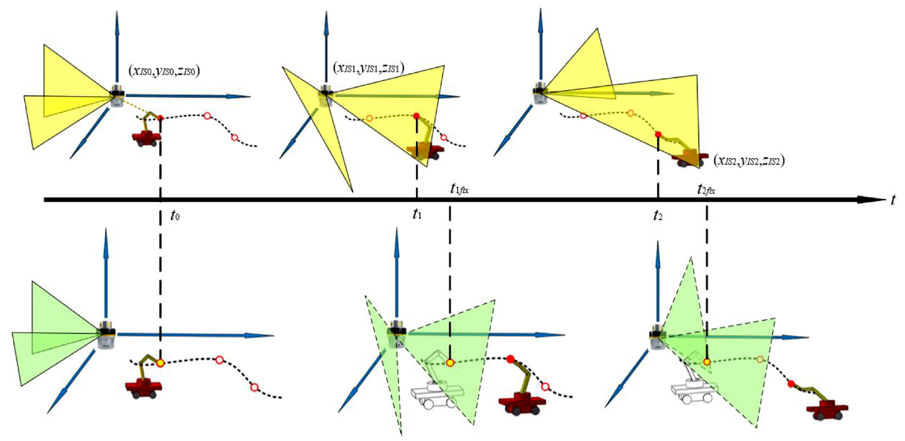
Schematic showing how the compensation algorithm operates when performing measurements using one transmitter.

The flow chart for the measurement result correction algorithm for the iGPS single-station measurement system is shown in Figure 4.

Figure 4.

Flow chart for the single transmitter compensation algorithm.

Mathematical model of correction algorithm for double station system

When two transmitters T₁ and T₂ are used to measure the moving target in turn, then the two measurement results are corrected according to the correction method proposed above, and the azimuth and elevation angles are obtained after the two measurements have been corrected. However, because of the movement of the target, the positions at which the two measurements are taken are not the same, which results in measurement uncertainty. We therefore use a similar method to correct the measurement results from the iGPS two-station measurement system. Using the correction algorithm for the single-station measurement system, we have calculated the times t_0(T1)(abs) and t_0(T2)(abs) for these two measurements on the absolute time axis. We can then calculate the equations of motion for the two fan beams of transmitter T₁ at time t_0(T1)(abs), as shown in equations (12) and (13):

F_{1 (T_{1})} (t_{1 (T_{1}) fix}) : {\begin{matrix} a_{1 (T_{1})} (t_{1 (T_{1}) fix}) \cdot x + b_{1 (T_{1})} (t_{1 (T_{1}) fix}) \cdot y + \\ c_{1 (T_{1})} (t_{1 (T_{1}) fix}) \cdot z = 0 \\ a_{1 ub (T_{1})} (t_{1 (T_{1}) fix}) \cdot x + b_{1 ub (T_{1})} (t_{1 (T_{1}) fix}) \cdot y \\ + c_{1 ub (T_{1})} (t_{1 (T_{1}) fix}) \cdot z \leq 0 \\ a_{1 lb (T_{1})} (t_{1 (T_{1}) fix}) \cdot x + b_{1 lb (T_{1})} (t_{1 (T_{1}) fix}) \cdot y \\ + c_{1 lb (T_{1})} (t_{1 (T_{1}) fix}) \cdot z \geq 0 \end{matrix}

(12)

F_{2 (T_{1})} (t_{2 (T_{1}) f i x}) : {\begin{matrix} a_{2 (T_{1})} (t_{2 (T_{1}) f i x}) \cdot x + b_{2 (T_{1})} (t_{2 (T_{1}) f i x}) \cdot y + \\ c_{2 (T_{1})} (t_{2 (T_{1}) f i x}) \cdot z = 0 \\ a_{2 u b (T_{1})} (t_{2 (T_{1}) f i x}) \cdot x + b_{2 u b (T_{1})} (t_{2 (T_{1}) f i x}) \cdot y \\ + c_{2 u b (T_{1})} (t_{2 (T_{1}) f i x}) \cdot z \leq 0 \\ a_{2 l b (T_{1})} (t_{2 (T_{1}) f i x}) \cdot x + b_{2 l b (T_{1})} (t_{2 (T_{1}) f i x}) \cdot y \\ + c_{2 l b (T_{1})} (t_{2 (T_{1}) f i x}) \cdot z \geq 0 \end{matrix}

(13)

Similarly, the equations for the two fan beams of transmitter T₂ at time t_0(T2)(abs) can be calculated as shown in equations (14) and (15).

F_{1 (T_{2})} (t_{1 (T_{2}) f i x}) : {\begin{matrix} a_{1 (T_{2})} (t_{1 (T_{2}) f i x}) \cdot x + b_{1 (T_{2})} (t_{1 (T_{2}) f i x}) \cdot y + \\ c_{1 (T_{2})} (t_{1 (T_{2}) f i x}) \cdot z = 0 \\ a_{1 u b (T_{2})} (t_{1 (T_{2}) f i x}) \cdot x + b_{1 u b (T_{2})} (t_{1 (T_{2}) f i x}) \cdot y \\ + c_{1 u b (T_{2})} (t_{1 (T_{2}) f i x}) \cdot z \leq 0 \\ a_{1 l b (T_{2})} (t_{1 (T_{2}) f i x}) \cdot x + b_{1 l b (T_{2})} (t_{1 (T_{2}) f i x}) \cdot y \\ + c_{1 l b (T_{2})} (t_{1 (T_{2}) f i x}) \cdot z \geq 0 \end{matrix}

(14)

F_{2 (T_{2})} (t_{2 (T_{2}) f i x}) : {\begin{matrix} a_{2 (T_{2})} (t_{2 (T_{2}) f i x}) \cdot x + b_{2 (T_{2})} (t_{2 (T_{2}) f i x}) \cdot y + \\ c_{2 (T_{2})} (t_{2 (T_{2}) f i x}) \cdot z = 0 \\ a_{2 u b (T_{2})} (t_{2 (T_{2}) f i x}) \cdot x + b_{2 u b (T_{2})} (t_{2 (T_{2}) f i x}) \cdot y \\ + c_{2 u b (T_{2})} (t_{2 (T_{2}) f i x}) \cdot z \leq 0 \\ a_{2 l b (T_{2})} (t_{2 (T_{2}) f i x}) \cdot x + b_{2 l b (T_{2})} (t_{2 (T_{2}) f i x}) \cdot y \\ + c_{2 l b (T_{2})} (t_{2 (T_{2}) f i x}) \cdot z \geq 0 \end{matrix}

(15)

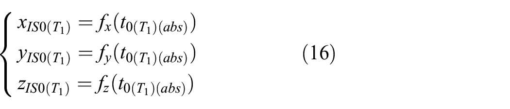
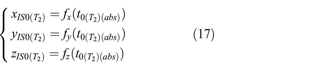
By substituting the times for these two measurements into the theoretical trajectory equation for the moving target, the theoretical coordinates of the moving target at these two moments are then obtained, as shown in equations (16) and (17).

{\begin{matrix} x_{IS 0 (T_{1})} = f_{x} (t_{0 (T_{1}) (abs)}) \\ y_{IS 0 (T_{1})} = f_{y} (t_{0 (T_{1}) (abs)}) \\ z_{IS 0 (T_{1})} = f_{z} (t_{0 (T_{1}) (abs)}) \end{matrix}

(16)

{\begin{matrix} x_{IS 0 (T_{2})} = f_{x} (t_{0 (T_{2}) (abs)}) \\ y_{IS 0 (T_{2})} = f_{y} (t_{0 (T_{2}) (abs)}) \\ z_{IS 0 (T_{2})} = f_{z} (t_{0 (T_{2}) (abs)}) \end{matrix}

(17)

When the measurement value at time t_0(T1)(abs) is taken as the criterion, then the measurement result for transmitter T₂ must be corrected, as shown in equation (18):

\begin{matrix} {\begin{matrix} a_{1 (T_{2})} (t_{1 (T_{2}) fix} + Δ {t_{1}}_{(T_{2})}) \cdot x_{IS 0 (T_{1})} + \\ b_{1 (T_{2})} (t_{1 (T_{2}) fix} + Δ {t_{1}}_{(T_{2})}) \cdot y_{IS 0 (T_{1})} + \\ c_{1 (T_{2})} (t_{1 (T_{2}) fix} + Δ {t_{1}}_{(T_{2})}) \cdot z_{IS 0 (T_{1})} = 0 \\ a_{2 (T_{2})} (t_{2 (T_{2}) fix} + Δ {t_{2}}_{(T_{2})}) \cdot x_{IS 0 (T_{1})} + \\ b_{2 (T_{2})} (t_{2 (T_{2}) fix} + Δ {t_{2}}_{(T_{2})}) \cdot y_{IS 0 (T_{1})} + \\ c_{2 (T_{2})} (t_{2 (T_{2}) fix} + Δ {t_{2}}_{(T_{2})}) \cdot z_{IS 0 (T_{1})} = 0 \end{matrix} \\ \to {\begin{matrix} t_{1 (T_{2}) {(fix)}^{2}} = t_{1 (T_{2}) fix} + Δ {t_{1}}_{(T_{2})} \\ t_{2 (T_{2}) {(fix)}^{2}} = t_{2 (T_{2}) fix} + Δ {t_{2}}_{(T_{2})} \end{matrix} \end{matrix}

(18)

Among these parameters, “(fix)²” indicates the secondary correction result obtained after application of the single-transmitter correction algorithm and the double-transmitter correction algorithm. Similarly, when the measurement value at time t_0(T2)(abs) is taken as the criterion, the measurement result for transmitter T₁ must be corrected, as shown in equation (19).

\begin{matrix} {\begin{matrix} a_{1 (T_{1})} (t_{1 (T_{1}) fix} + Δ {t_{1}}_{(T_{1})}) \cdot x_{IS 0 (T_{2})} + \\ b_{1 (T_{1})} (t_{1 (T_{1}) fix} + Δ {t_{1}}_{(T_{1})}) \cdot y_{IS 0 (T_{2})} + \\ c_{1 (T_{1})} (t_{1 (T_{1}) fix} + Δ {t_{1}}_{(T_{1})}) \cdot z_{IS 0 (T_{2})} = 0 \\ a_{2 (T_{1})} (t_{2 (T_{1}) fix} + Δ {t_{2}}_{(T_{1})}) \cdot x_{IS 0 (T_{2})} + \\ b_{2 (T_{1})} (t_{2 (T_{1}) fix} + Δ {t_{2}}_{(T_{1})}) \cdot y_{IS 0 (T_{2})} + \\ c_{2 (T_{1})} (t_{2 (T_{1}) fix} + Δ {t_{2}}_{(T_{1})}) \cdot z_{IS 0 (T_{2})} = 0 \end{matrix} \\ \to {\begin{matrix} t_{1 (T_{1}) {(fix)}^{2}} = t_{1 (T_{1}) fix} + Δ {t_{1}}_{(T_{1})} \\ t_{2 (T_{1}) {(fix)}^{2}} = t_{2 (T_{1}) fix} + Δ {t_{2}}_{(T_{1})} \end{matrix} \end{matrix}

(19)

Thus far, when it has been necessary to use the measurement from one transmitter as the standard, the correction algorithm for the measurement value from the other transmitter has been obtained and the corrected azimuth and elevation have been calculated based on the principle of convergence. The corrected coordinate values of the moving target are then finally calculated. Figure 5 provides a clear illustration of the principle of the iGPS two-station system correction algorithm.

Figure 5.

Schematic showing how the compensation algorithm operates when performing measurements using two transmitters.

The flow chart for the measurement result correction algorithm for the iGPS double-station measurement system is shown in Figure 6.

Figure 6.

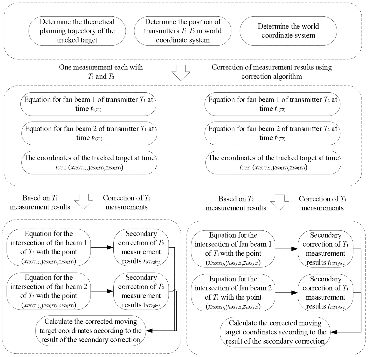
Flow chart for the double transmitter compensation algorithm.

Simulation test and results analysis

Simulation environment construction and test plan formulation

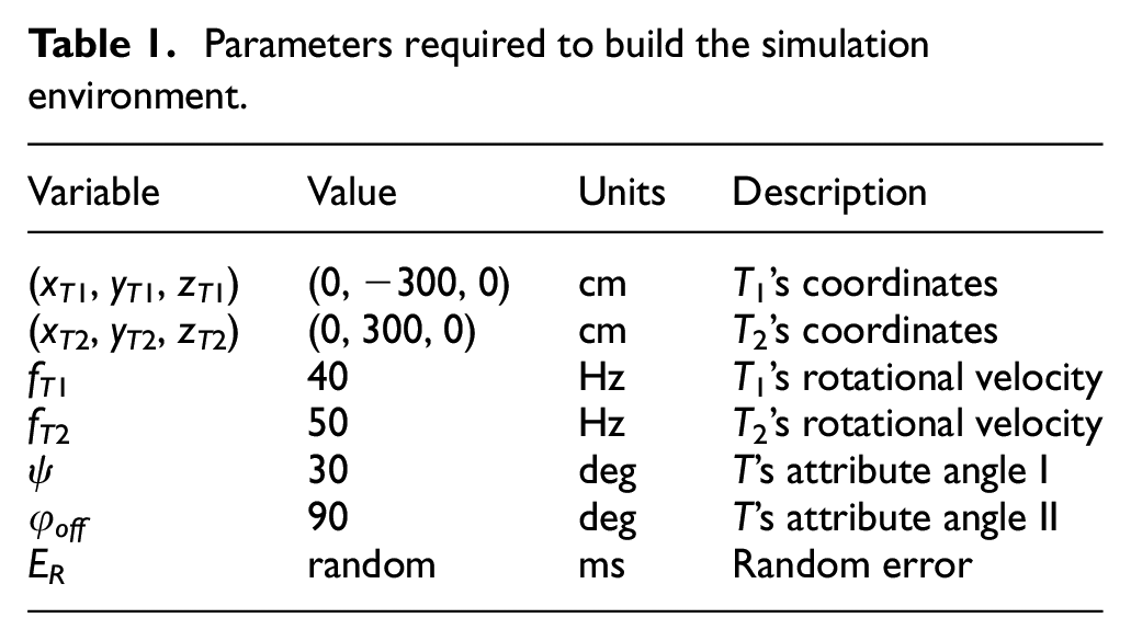
To verify the correctness of the correction algorithm, we began by conducting simulation experiments on the correction algorithm. The simulation environment was built in MATLAB (Mathworks). The environmental parameters included the coordinates of the transmitter in the global coordinate system, the rotation frequency of the transmitter head, the geometric characteristics of the fan beam emitted by the transmitter, and the random errors that occur during normal measurement processes. A detailed description and the specific values of the environmental parameters of the simulation environment are presented in Table 1.

Table 1.

Parameters required to build the simulation environment.

Variable	Value	Units	Description
(x_T₁, y_T₁, z_T₁)	(0, −300, 0)	cm	T ₁’s coordinates
(x_T₂, y_T₂, z_T₂)	(0, 300, 0)	cm	T ₂’s coordinates
f_T ₁	40	Hz	T ₁’s rotational velocity
f_T ₂	50	Hz	T ₂’s rotational velocity
ψ	30	deg	T’s attribute angle I
φ_off	90	deg	T’s attribute angle II
E_R	random	ms	Random error

In the simulation environment, we can assume that the receiver is completely coincident with the tracked target, ensure that the tracked target moves according to a specific theoretical curve, and use the transmitter to measure the tracked target. To verify that the proposed algorithm is suitable for use with different motion trajectories, we use three types of curve to test the algorithm, comprising a 1D straight line, a 2D sinusoidal curve, and a 3D spiral. At the same time, to verify the robustness of the algorithm and prove its invariance with respect to the direction and orientation of the trajectory in space, we consider the cases where the one-dimensional straight line is directed along the x-axis, the y-axis, and the z-axis; the cases where the two-dimensional sinusoid is located on the xoy plane, the xoz plane, and the yoz plane; and the cases where the axes for the three-dimensional spiral are oriented along the x-axis, the y-axis, and the z-axis. Finally, to verify the sensitivity of the proposed algorithm to the speed of the tracked target, we let the tracked target move at speeds of 10, 20, 30, 40, and 50 mm/s. A total of 200 points per trial were measured using the transmitter.

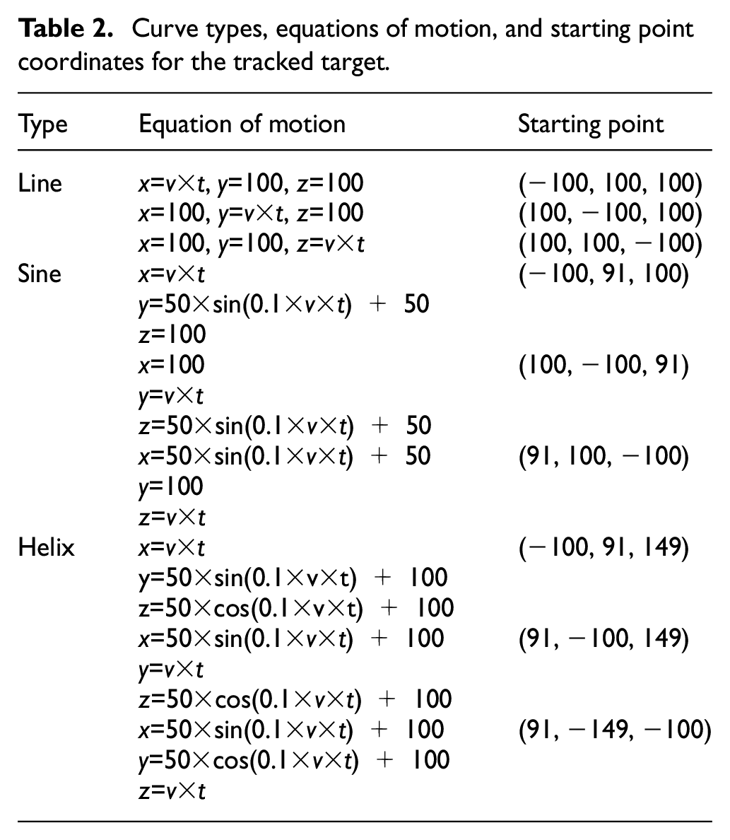
The test curve, the motion equation, and the starting point coordinates are presented in Table 2.

Table 2.

Curve types, equations of motion, and starting point coordinates for the tracked target.

Type	Equation of motion	Starting point
Line	x=v×t, y=100, z=100	(−100, 100, 100)
	x=100, y=v×t, z=100	(100, −100, 100)
	x=100, y=100, z=v×t	(100, 100, −100)
Sine	x=v×t y=50×sin(0.1×v×t) + 50 z=100	(−100, 91, 100)
	x=100 y=v×t z=50×sin(0.1×v×t) + 50	(100, −100, 91)
	x=50×sin(0.1×v×t) + 50 y=100 z=v×t	(91, 100, −100)
Helix	x=v×t y=50×sin(0.1×v×t) + 100 z=50×cos(0.1×v×t) + 100	(−100, 91, 149)
	x=50×sin(0.1×v×t) + 100 y=v×t z=50×cos(0.1×v×t) + 100	(91, −100, 149)
	x=50×sin(0.1×v×t) + 100 y=50×cos(0.1×v×t) + 100 z=v×t	(91, −149, −100)

Analysis and discussion of simulation test results

Figures 7, 8, and 9 show the results of the simulation tests. Each figure includes three images, which represent the same type of curve for the three different motion directions in each case. To show the results of the simulation tests intuitively, the measurement points before correction, the measurement points after correction, and the theoretical trajectory of the tracked target are all shown within the same figure in each case. In each figure, the black dotted line represents the theoretical trajectory of the tracked target’s movement, the darker colored dots represent the measurement points before correction, and the lighter colored points represent the corrected measurement points. To allow each figure to express the relevant information clearly and comprehensively, each motion trajectory is divided into five parts, where each part expresses when the tracked object moves according to the motion trajectory at the different speeds (10, 20, 30, 40, and 50 mm/s), and shows the distributions of the measurement results before correction and after correction.

Figure 7.

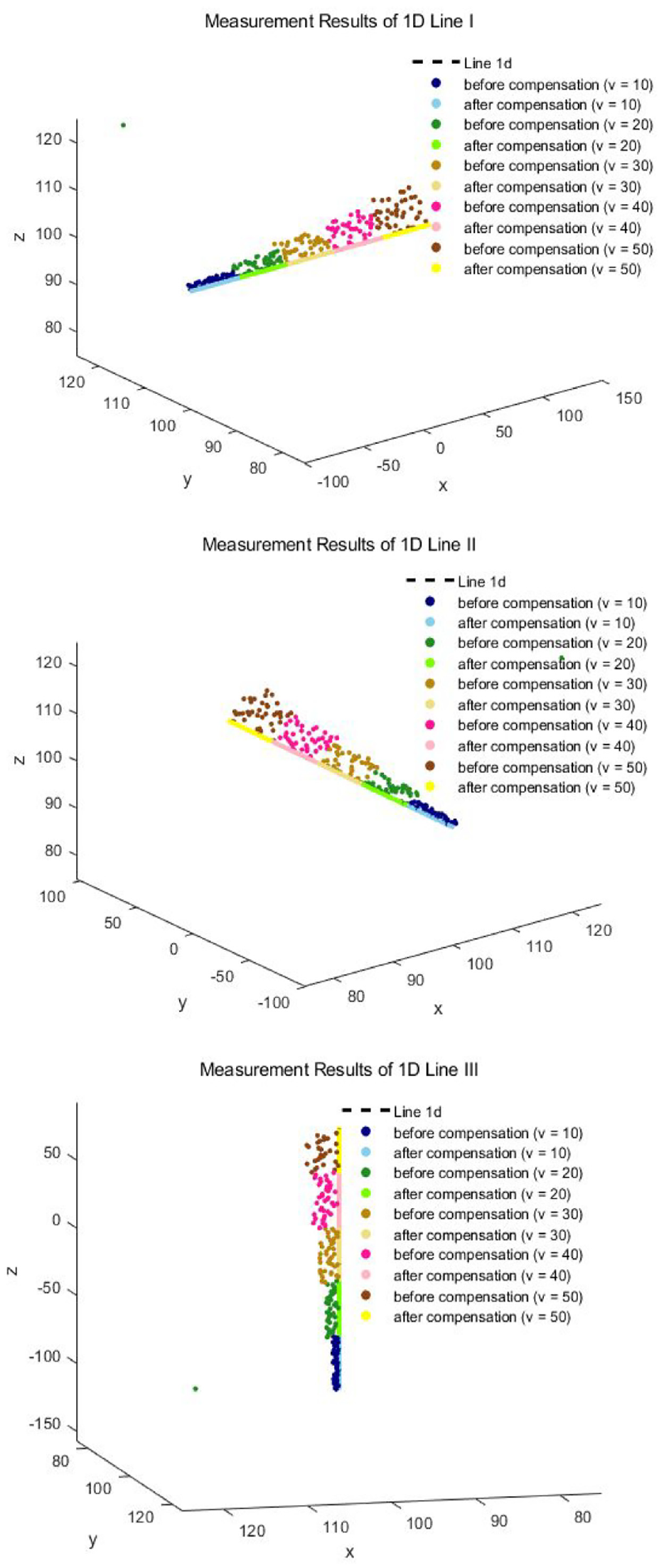
Measurement results for the linear motion trajectory.

Figure 8.

Measurement results for the sinusoidal motion trajectory.

Figure 9.

Measurement results for the helical trajectory.

Figures 10, 11, and 12 show the variations in the errors for the measurement results (i.e., the Euclidean distance between the measurement result and the theoretical trajectory in each case) with respect to the movement speed of the tracked target and the degree of fluctuation that occurs at different times when the iGPS measurement system is tracking trajectory curves with different complexities.

Figure 10.

Errors in the linear motion trajectories (before compensation and after compensation).

Figure 11.

Errors in the sinusoidal motion trajectories (before compensation and after compensation).

Figure 12.

Errors in the helical motion trajectories (before compensation and after compensation).

Tables 3 and 4 detail the main statistical features of the simulation results.

Table 3.

Statistical features of the simulation results for the different trajectory types.

Statistical features of the errors	Trajectory Type
Statistical features of the errors	Line	Sine	Helix
Mean (BC)	2.5319	10.5211	12.5818
STD (BC)	1.6087	8.5876	8.8108
Median (BC)	2.3169	8.3583	8.0396
Mean (AC)	0.0078	0.0062	0.0083
STD (AC)	0.0066	0.0030	0.0091
Median (AC)	0.0061	0.0057	0.0057

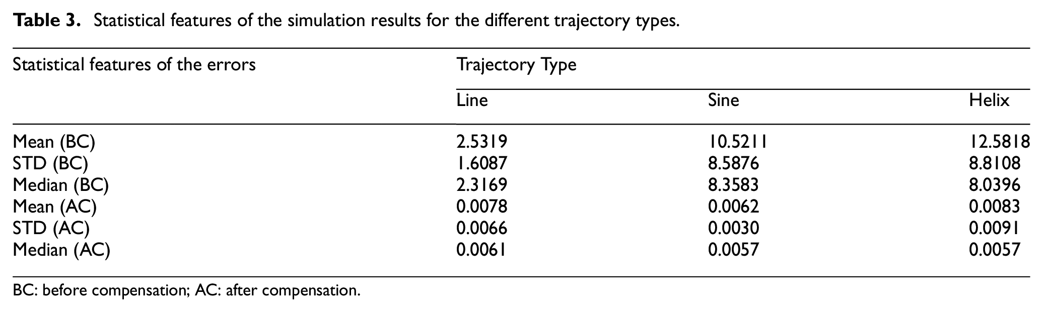
BC: before compensation; AC: after compensation.

Table 4.

Statistical features of the simulation results for the different target velocities.

Statistical features of errors	Velocity of the tracked target (mm/s)
Statistical features of errors	10	20	30	40	50
Mean (BC)	2.82	5.56	7.49	10.77	12.77
STD (BC)	2.62	4.74	6.21	9.52	10.31
Median (BC)	2.02	4.09	5.56	7.89	10.17
Mean (AC, 10⁻³)	5.8	6.0	5.9	5.9	5.3
STD (AC, 10⁻³)	7.6	7.5	8.1	7.5	6.4
Median (AC, 10⁻³)	3.5	3.8	3.4	3.5	3.6

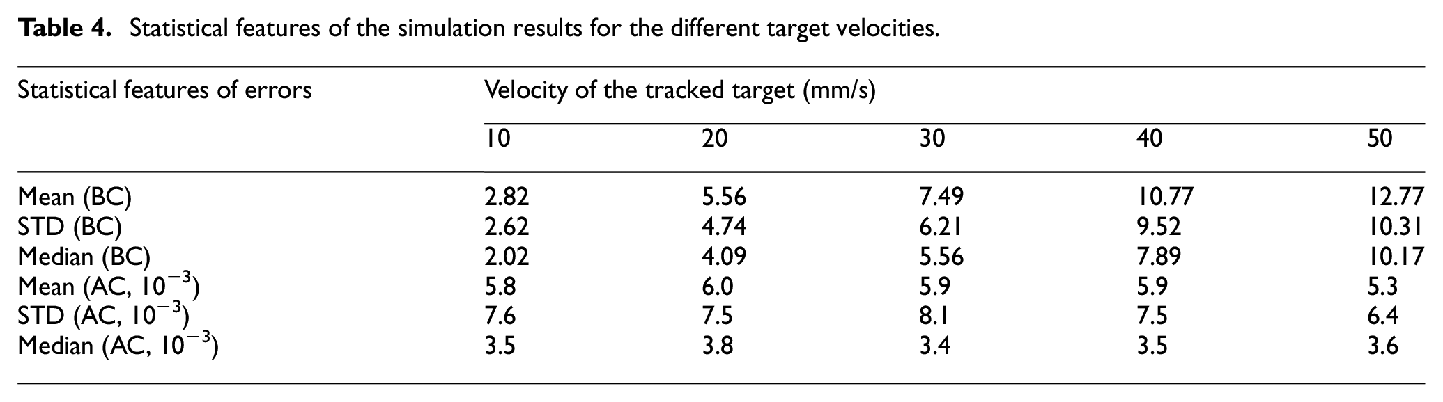
From the simulation experiment results and the data statistics, we found that the measurement uncertainty and the degree of fluctuation in the measurements from the iGPS measurement system will increase with acceleration in the speed of movement of the tracked target and with increases in the complexity of the movement curve, which is in line with existing cognitive laws. The simulation correction algorithm proposed in this work not only greatly reduces the errors and improves the measurement stability, but also is hardly affected by the object’s speed or the complexity of the trajectory. The validity of the modified algorithm is thus confirmed.

Conclusion

Use of an iGPS measurement system in industrial production is relatively common, but when the iGPS is used to track a target dynamically, the measurement accuracy will decrease. After in-depth research into the measurement principle of the iGPS measurement system, we have proposed a compensation algorithm to compensate the data obtained via iGPS dynamic tracking measurements when using iGPS to track a dynamic target. This method mainly uses the motion equation for the infrared signal of the transmitter and the theoretical equation for the moving target as a basis on which to compensate for the position of the moving object and then compensate the measured data. We used MATLAB to build a suitable simulation environment and then selected representative one-dimensional curves, two-dimensional curves, and three-dimensional curves to test the proposed algorithm. After testing, the algorithm proposed in this paper can improve the tracking and measurement accuracy of the iGPS measurement system effectively for use with dynamic targets. It should be noted that this algorithm is more suitable for situations in which there is no obvious deviation in the track of the tracked target, but where the tracked target shows obvious overspeed or delay characteristics.

Research Data

sj-xlsx-1-ade-10.1177_16878132231170771 – Supplemental material for Research on the Method of Improving iGPS Dynamic Tracking Accuracy Based on Theoretical Trajectory Backward Compensation

Supplemental material, sj-xlsx-1-ade-10.1177_16878132231170771 for Research on the Method of Improving iGPS Dynamic Tracking Accuracy Based on Theoretical Trajectory Backward Compensation by Rui Han, Erik Trostmann and Thomas Dunker in Advances in Mechanical Engineering

This article is distributed under the terms of the Creative Commons Attribution 4.0 License (https://creativecommons.org/licenses/by/4.0/) which permits any use, reproduction and distribution of the work without further permission provided the original work is attributed as specified on the SAGE and Open Access pages (https://us.sagepub.com/en-us/nam/open-access-at-sage).

Supplemental Material

sj-rar-2-ade-10.1177_16878132231170771 – Supplemental material for Research on the Method of Improving iGPS Dynamic Tracking Accuracy Based on Theoretical Trajectory Backward Compensation

Supplemental material, sj-rar-2-ade-10.1177_16878132231170771 for Research on the Method of Improving iGPS Dynamic Tracking Accuracy Based on Theoretical Trajectory Backward Compensation by Rui Han, Erik Trostmann and Thomas Dunker in Advances in Mechanical Engineering

Footnotes

Correction (July 2023):

The affiliations of the authors have been reordered and the affiliations of Rui Han have been updated.

Handling Editor: Chenhui Liang

Declaration of conflicting interests

The author(s) declared no potential conflicts of interest with respect to the research, authorship, and/or publication of this article.

Funding

The author(s) disclosed receipt of the following financial support for the research, authorship, and/or publication of this article: This work was supported by the European Regional Development Fund (ERDF) and the state of Saxony-Anhalt (ZWB: 2004/00070 | Laufzeit: 01.08.2020-30.04.2022).

ORCID iD

Rui Han

Supplemental material

Supplemental material for this article is available online.

References

Chen

Fang

. Intelligentized technologies for welding manufacturing. In: Kiet Tieu

Zhu

(eds) Materials science forum (vols. 773–774). Switzerland: Trans Tech Publications, 2013, pp. 725–731.

Zhou

. Digitalization and intelligentization of manufacturing industry. Adv Manuf 2013; 1: 1–7.

Mei

Maropoulos

. Review of the application of flexible, measurement-assisted assembly technology in aircraft manufacturing. Proc Inst Mech Eng B J Eng Manuf 2014; 22. Epub ahead of print 7 February 2014. DOI: 10.1177/0954405413517387.

Liu

Xie

, et al. Laser tracker based robotic assembly system for large scale peg-hole parts. In: 2014 IEEE 4th annual international conference on cyber technology in automation, control, and intelligent systems (CYBER), Hong Kong, 4–7 June 2014, pp. 574–578. New York: IEEE.

Zhang

Shi

. A dimensional measurement method based on a laser tracker for a crane assembly. Laser Eng 2013; 26: 91–101.

Peggs

Maropoulos

Hughes

, et al. Recent developments in large-scale dimensional metrology. Proc Inst Mech Eng B J Eng Manuf 2009; 223: 571–596.

Muelaner

Wang

Jamshidi

, et al. Study of the uncertainty of angle measurement for a rotary-laser automatic theodolite (R-LAT). Proc Inst Mech Eng B J Eng Manuf 2009; 223; 217–229.

Hao

Yin

, et al. Research on the IGPS device error and its influence of positioning accuracy. In: IEEE forum on cooperative positioning and service (CPGPS), Harbin, China, 19–21 May 2017, pp. 294–299. New York: IEEE.

Landeta

Sutério

Gonzaga Trabasso

. Metrological comparison between two sensor-configurations of the IGPS measurement system. In: ABCM symposium series in mechatronics, Natal, Brazil, 24–28 October 2011, pp. 1319–1328. Lisbon: ABCM.

10.

Maisano

Jamshidi

Franceschini

, et al. Indoor GPS: system functionality and initial performance evaluation. Int J Manuf Res 2008; 3: 335–349.

11.

Zhou

, et al. iGPS Measurement network multi-station arrangement design. Appl Mech Mater 2014; 443: 223–227.

12.

Depenthal

Schwendemann

. IGPS–A new system for static and kinematic measurements. In: Optical 3-D measurement techniques IX (eds. Grün

Kahmen

), Vienna, Austria, 1–3 July 2009, pp. 131–140.

13.

Heiden

Porath

. Metrological performance of iGPS in measurement assisted assembly process. In: 8th Brazilian congress on metrology, Bento Gonçalves, Brazil, 6–8 September 2015, pp. 356–363.

14.

Wang

Mastrogiacomo

Franceschini

, et al. Experimental comparison of dynamic tracking performance of iGPS and laser tracker. Int J Adv Manuf Technol 2011; 56: 205–213.

15.

Depenthal

. Path tracking with iGPS. In: IEEE international conference on indoor positioning and indoor navigation (IPIN), Zurich, Switzerland, 15–17 September 2010, pp. 1–6. New York: IEEE.

16.

Zhao

Jing

Chen

, et al. Dynamic tracking performance of indoor global positioning system: An experimental and theoretical study. Adv Mech Eng 2015; 7: 1–8.

17.

Zeng

Huang

, et al. High-efficiency posture prealignment method for large component assembly via iGPS and laser ranging. IEEE Trans Instrum Meas 2020; 69: 5497–5510.

18.

Schmitt

Kimmelman

Quinders

, et al. Investigation of the applicability of an iGPS metrology system to automate the assembly in motion of a trunk cabin. Appl Mech Mater 2016; 840: 58–65.

19.

Chen

Tang

Yang

, et al. Study and application of lunar rover tracking measurement technology with laser radar and iGPS. In: International conference on manufacturing technology, Wuhan, China, 14–16 June 2019, pp. 592–599. Bristol: IOP Publishing.

Supplementary Material

Please find the following supplemental material available below.

For Open Access articles published under a Creative Commons License, all supplemental material carries the same license as the article it is associated with.

For non-Open Access articles published, all supplemental material carries a non-exclusive license, and permission requests for re-use of supplemental material or any part of supplemental material shall be sent directly to the copyright owner as specified in the copyright notice associated with the article.

0.00 MB

0.07 MB

0.81 MB