
Abstract
Articulated tracked vehicles are used as special off-road transportation vehicles, and their mobility is gaining more attention now than before. As an important evaluation indicator of the mobility of articulated tracked vehicles, steering performance receives wide attention in particular. Most of the present studies focus on the planar steering performance; few studies employing current models concentrate on the slope steering performance of articulated tracked vehicles. To address this research gap, this study proposes a dynamic modeling method for analyzing the slope steering performance of articulated tracked vehicles. A kinematic model of a vehicle is initially constructed to analyze its kinematic characteristics during slope steering; these characteristics include velocity and acceleration. A dynamic model of a vehicle is then developed to analyze its mechanical characteristics during slope steering; these characteristics include vertical loads, driving forces, and driving moments of tracks. The created dynamic model is then applied to analyze the slope steering performance of a specific articulated tracked vehicle. A mechanical-control united simulation model and an actual test of an articulated tracked vehicle are suggested to verify the established steering model. Comparison results show the effectiveness of the proposed dynamic steering model.
Keywords
Introduction
Articulated tracked vehicles are recently developed as special engineering vehicles, and they are widely applied in various engineering fields, such as military, agriculture, and forestry transport.1,2
As an important evaluation indicator of mobility of tracked vehicles, steering performance causes much public concern.3–5 Bekker 6 studied the driving performance of tracked vehicles on soft terrain, and his works involved steering performance, vertical pressure soil sinkage relations at the track–ground interface, and passability evaluation. Wong and colleagues7–9 expanded Bekker’s theory and proposed a series of methods to study the steering performance of tracked vehicles. Wang et al. 10 studied the tractive performance of seafloor tracked trencher. Yao et al. 11 proposed a novel method for estimating the track–soil parameters at the track–ground interface. Wang et al. 12 comprehensively studied the steering performance of armored vehicles based on experiments. Kapania and Gerdes 13 designed a feedback–feedforward steering controller for accurate path tracking. Salehpour et al. 14 developed a new vehicle path tracking algorithm with integrated chassis control. The aforementioned works3–14 mainly focus on studying the steering performance of a traditional single-tracked vehicle or the control algorithm of motion path. These methods are not employed in research on articulated tracked vehicles.
The steering manner of articulated tracked vehicles differs from that of traditional single-tracked vehicles. Therefore, the developed methods3–14 cannot be directly used to analyze the steering ability of articulated tracked vehicles.
Currently, only a limited number of studies are conducted on the steering performances of multi-tracked vehicles. Watanabe and Kitano 15 presented a planar steering model of articulated tracked vehicles. Williams 16 studied the handling ability of a multi-axle vehicle. Ding and Guo 17 developed a generalized equivalent estimation approach to analyze the handling dynamics of multi-axle vehicles. Yao et al. 18 studied the steering performances of six tracked vehicles. The above methods15–18 are used to study the steering performances of multi-tracked or articulated tracked vehicles on planes; these methods cannot be utilized to analyze the steering performances of articulated tracked vehicles on ramp surfaces. Zhang et al. 19 studied the control strategy of the flexible steering system of an all-wheel-steering robot. Norouzi et al. studied the control strategies of multi-tracked vehicles. 20 These two methods19,20 only discuss the controlling strategies of movement trajectory; the mechanical characteristics of tracks or tires during steering process are not studied.
Current models are designed for studying the steering abilities of traditional single-tracked vehicles,3–14 or they only emphasize the planar steering performances of multi-tracked or articulated tracked vehicles15–18 or analyze motion trajectory planning.19,20 Such research gap should be addressed, given that the road conditions of articulated tracked vehicles are worse than that of single-tracked vehicles. Articulated tracked vehicles often encounter extreme terrain conditions (e.g. trenches, upland, and jungle area) in actual engineering practice. Articulated tracked vehicles also frequently experience steering movement on ramp surfaces. Therefore, a dynamic modeling method for analyzing the slope steering performance of articulated tracked vehicles is urgently needed to develop the driving mechanics of articulated tracked vehicles.
To fill the aforementioned research gaps, this study proposes a dynamic modeling method for analyzing the slope steering performance of articulated tracked vehicles. This model is composed of kinematic, dynamic, and track–soil sub-models. The slope steering performance of a specific articulated tracked vehicle is thoroughly investigated by adopting the established theoretical model as well as conducting a virtual prototype simulation and an actual testing of an articulated tracked vehicle.
Movement mechanism of the articulated unit during slope steering
Articulated tracked vehicles complete the slope steering motion by controlling the posture of the articulated unit. When vehicles turn left, the left steering hydraulic cylinder is in a contraction state and the right steering hydraulic cylinder is in an elongation state (Figure 1(a)). The left and right steering hydraulic cylinders do not elongate or shorten when vehicles are not steering (Figure 1(b)). When vehicles turn right, the left steering hydraulic cylinder is in an elongation state and the right steering hydraulic cylinder is in a contraction state (Figure 1(c)).

Posture variation of the articulated unit during slope steering: (a) vehicles turn left, (b) vehicles are not steering, and (c) vehicles turn right.
The driving movements provided by the steering hydraulic cylinders during slope steering can be expressed as
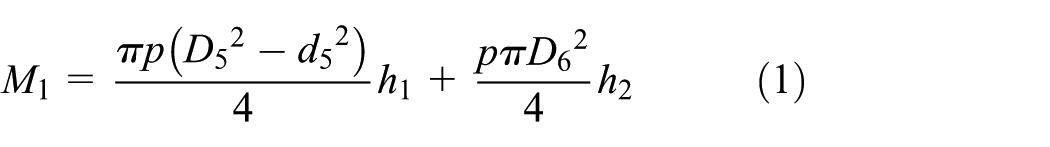

where M1 is the driving moment when vehicles turn left, M2 is the driving moment when vehicles turn right, p is the output oil pressure of the steering hydraulic cylinders, D5 and D6 are the diameters of the left and right steering hydraulic cylinders, respectively, d5 and d6 are the diameters of the piston rods of the left and right steering hydraulic cylinders, respectively, and h1, h2, h3, and h4 are the arms of force with respect to O for the steering hydraulic cylinders, as shown in Appendix 2.
Table 1 lists the structure parameters of the articulated unit.
Structure parameters of the articulated unit.

The data in Table 1 are integrated into formulas (1) and (2). The mechanical parameters of the articulated unit during slope steering are then calculated (Table 2).
Computational results of the mechanical parameters of the articulated unit according to the theoretical model.

Kinematic model of articulated tracked vehicles during slope steering
To facilitate the study, the following assumptions are retained:
An articulated tracked vehicle is performing the steady steering movement on a ramp surface.
The ramp surface is a plane.
The influence of centrifugal force on the vehicle steering performance is not considered.
Track pressure is continuous in a linear variation.
The effect of pitching and roll motion on the steering performance is not considered.
To expediently describe the pose of articulated tracked vehicles during slope steering, the following coordinate systems are established:
The world coordinate system of Ow5-x5y5z5;
The coordinate system of the ramp surface of Os1-x4y4z4, in which Os1 is the steering center;
The coordinate systems of the front and rear vehicles of O1-x1y1z1 and O3-x3y3z3, in which O1 and O3 are the geometric centers of the front and rear vehicle projection on the ramp surface.
Figure 2 depicts the kinematic model of articulated tracked vehicle during steady slope steering. Os1 is the steering center, R1 is the steering radius of vehicle,

Kinematic model of articulated tracked vehicle when the vehicle is steering on a ramp surface.
Figure 3 depicts the motion vector relationships of all coordinate systems during slope steering. In this process, the pose of O1-x1y1z1 and O3-x3y3z3 experiences two changing phases. In the first phase, when the vehicle moves from the plane to the ramp surface, the y- and z-axle of the O1-x1y1z1 and O3-x3y3z3 rotate α° around the own x-axle. In the second phase, when the vehicle is steering around the Os1 on the ramp surface, the x- and y-axle of the O1-x1y1z1 and O3-x3y3z3 rotate θ° around the own z-axle.
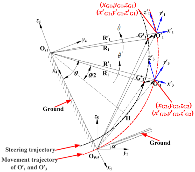
Motion vector relationships of all coordinate systems.
According to the relations in Figure 3, under the Ow5-x5y5z5, the positions of
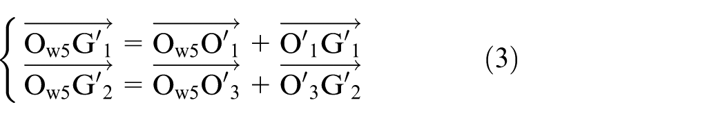
where the vectors of
According to the relations in Figure 3, the vectors of
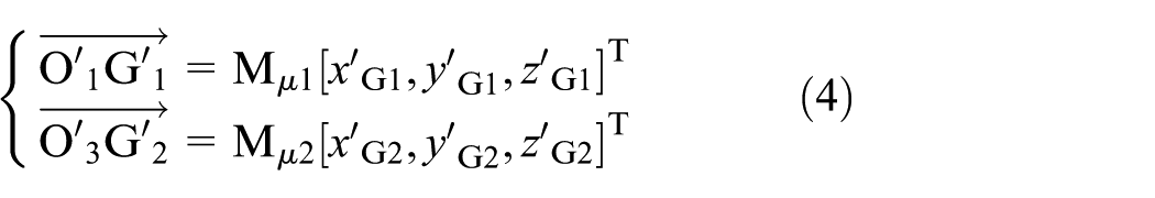
where
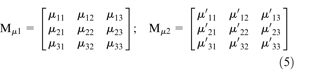
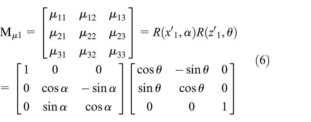
where µmn (m = n = 1, 2, 3) are the direction cosine of angles between the coordinate axis of
Using the homogeneous coordinate transformation method, Mµ1 and Mµ2 can be acquired as follows

where
Using the homogeneous coordinate transformation method, the vectors of
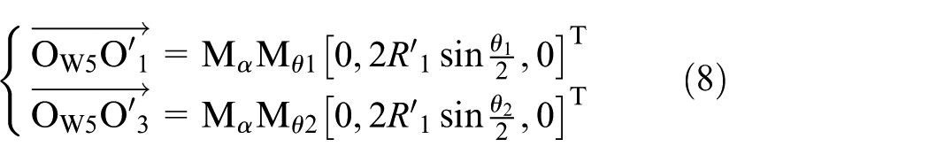
where M α Mθ1 and M α Mθ2 are the homogeneous coordinate transformation matrices, which are expressed as follows

where θ1 and θ2 are the azimuth angles of the front and rear vehicles. During steady slope steering, the azimuth angles of the front and rear vehicles should be the same with the azimuth angle of the articulated tracked vehicle. Therefore, θ1 = θ2 = θ.
Then, substituting formulas (4)–(9) into formula (3), the coordinate values of
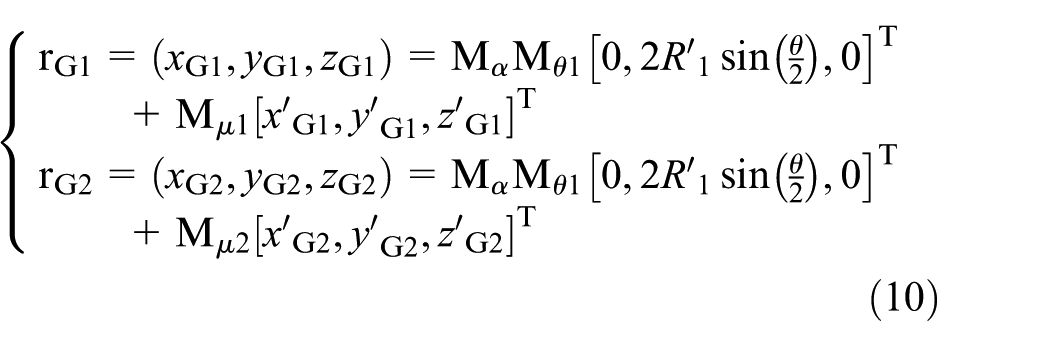
where

The steering angle and acceleration of vehicles during slope steering can be expressed as follows

where vk is the velocity of the front and rear vehicles during slope steering and ak is the acceleration of the front and rear vehicles in the process.
Formula (10) is a function of θ, and θ is a variable that varies as the time of t changes. Therefore, the velocities and accelerations of the centers of gravity for the front and rear vehicles (G1 and G2) under the world coordinate system of Ow5-x5y5z5 can be obtained using the derivation method, as shown in Appendix 4.
Dynamic model of articulated tracked vehicles during slope steering
Mechanical characteristics of articulated tracked vehicles
Figure 4 depicts the mechanical conditions of articulated tracked vehicles during slope steering. In this process, the mechanical conditions of vehicle are mainly the gravity of vehicle, the friction resisting forces from the soft terrain, the inertia force of the vehicle, and the supporting forces from the ground. When the vehicle is performing the steady steering movement, all external forces should remain balanced with respect to O1 and O3.
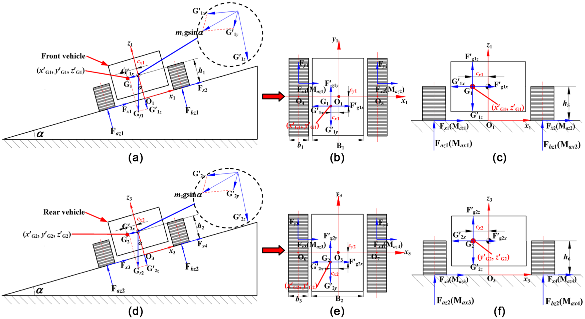
Mechanical conditions of articulated tracked vehicles during slope steering: (a) mechanical conditions of front vehicle on the ramp surface, (b) mechanical conditions of the front vehicle in the coordinate plane of O1-x1o1y1, (c) mechanical conditions of the front vehicle in the coordinate plane of O1-x1o1z1, (d) mechanical conditions of rear vehicle on the ramp surface, (e) mechanical conditions of the rear vehicle in the coordinate plane of O3-x3o3y3, and (f) mechanical conditions of the rear vehicle in the coordinate plane of O3-x3o3z3.
According to the mechanical relations in Figure 4, the components of gravity for the front and rear vehicles in xs, ys, and zs (s = 1, 3) directions under O1-x1o1y1 and O3-x3o3y3, respectively, can be expressed as

where m1 and m2 are the qualities of the front and rear vehicles, g is the acceleration of gravity, and g = 9.8 m/s 2 .
The inertia forces of the front and rear vehicles during slope steering under O1-x1y1z1 and O3-x3y3z3, respectively, can be expressed as
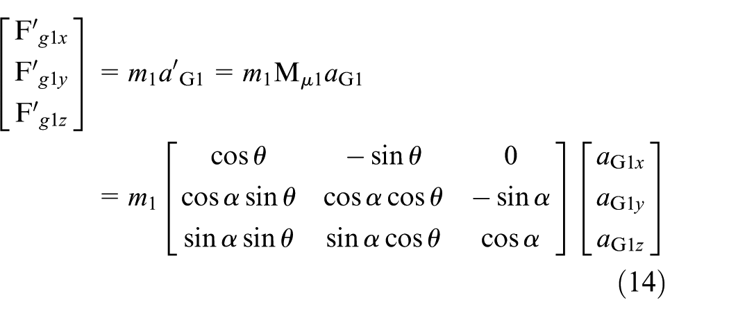

where m1 and m2 are the mass of the front and rear vehicle units, Mµ1 and Mµ2 are the homogeneous coordinate transformation matrices, as given in formulas (6) and (7),
The inertia moments of revolution with respect to the z1- and z3-axle for the front and rear vehicles during slope steering under O1-x1y1z1 and O3-x3y3z3, respectively, can be expressed as

where
Here, the mechanical analysis of the front vehicle is taken as an example. According to the mechanical relations in Figure 4, the following mechanical equilibrium equations are derived

where Fx1 and Fx2 are the lateral resisting forces of the inner and outer tracks; Fy1 is the braking force of the inner track; Fy2 is the tractive force of the outer track;
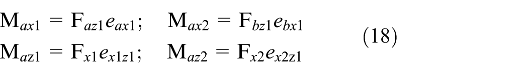
where µ is the friction coefficient between the track and the soil, Faz1 and Fbz1 are the average vertical loads of the inner and outer tracks for the front vehicle, respectively, eax1 and ebx1 are the longitudinal deviations of the average vertical loads of the inner and outer tracks of Faz1 and Fbz1, respectively, and ex1z1 and ex2z1 are the longitudinal deviations of the lateral resisting forces of the inner and the outer tracks of Fx1 and Fx2 with respect to the z1-axle, respectively.
During steady steering, the torsion angles of revolution with respect to x1-axle for the inner and outer tracks should be equal, which results in the following equation
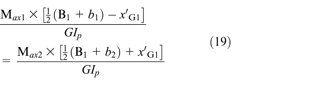
where GIp is the torsional stiffness of the front vehicles and

where h5 and h6 are the heights of the pressure centers of gravity of G1 and G2.
By simultaneously solving formulas (17)–(19), the average vertical loads of the inner and outer tracks for the front vehicle (Faz1, Fbz1), as shown in Appendix 5, and the longitudinal deviation of the average vertical loads of the inner and outer tracks for the front vehicle (eax1, ebx1), as shown in Appendix 6, can be obtained.
The average vertical loads of the inner and outer tracks for the rear vehicle (Faz2, Fbz2) and the longitudinal deviation of the average vertical loads of the inner and outer tracks for the rear vehicle (eax2, ebx2) can be obtained in the same way. The former is shown in Appendix 5, and the latter is shown in Appendix 6.
Track pressure distribution at the track–ground interface
Figure 5 shows the lateral force conditions of articulated tracked vehicles and the pressure distribution of track during slope steering. Figure 5 indicates that due to the lateral and longitudinal deviations of the pressure centers of the front and rear vehicles (G1 and G2) during slope steering, the pressures of the inner and outer tracks present an evidently uneven distribution, as shown in Figure 5(a)–(c), and then affect the lateral force distributions of tracks. Therefore, the lateral forces of F xi , (i = 1, 2, 3, 4), also presents an evidently uneven distribution.

Vehicle lateral force conditions and track pressure distribution during steering on a ramp surface: (a) the first track pressure distribution style, (b) the second track pressure distribution style, and (c) the third track pressure distribution style.
The average pressure of the inner and outer tracks at the track–ground interface can be expressed as follows

where b i is the width of tracks and L i is the length of tracks. F azk and F bzk are the average vertical loads of the inner and outer tracks, as shown in Appendices 5 and 6, respectively.
According to the mechanical relations in Figure 5, the following mechanical equations are derived
where qok and
By solving formula (22), the front- and rear-end pressures of the inner and outer tracks for the front and rear vehicles at the track–ground interface during slope steering can be expressed as follows

1. The first pressure distribution type of the inner and outer tracks, as shown in Figure 5(a), is given as follows.
The front- and rear-end pressures of the inner and outer tracks meet the following conditions

According to the assumptions above, the track pressures are continuous in a linear variation. Therefore, the functions of the pressures for the inner and outer tracks (equations of straight lines of AB and A′B′) under Os-ysOszs (s = 1, 3) are set as

The coordinate values of A, B, A′, and B′ under O1-y1O1z1 in Figure 5(a) are (−L
i
/2, qak), (L
i
/2, qbk), (−L
i
/2,
Then, the coordinate values of A, B, A′, and B′ are substituted in formula (25). The first pressure distribution type of the inner and outer tracks at point (xi, yi) can be expressed as follows

2. Using the same method similar to solving the first pressure distribution style of the inner and outer tracks, the second and third pressure distribution types of the inner and the outer tracks (P3(xi, yi), P4(xi, yi), P5(xi, yi), and P6(xi, yi)) in Figure 5(b) and (c) can be obtained, as shown in Appendix 7.
Soil–track interactional relationship
Figure 6 presents the soil–track interaction relation during slope steering. According to Wong’s theory, soil deformation experiences three stages: (1) plastic deformation stage, (2) plastic–elastic deformation stage, and (3) elastic deformation stage. The first stage occurs in the region between A and B; in this area, soil deformation mainly generates plastic deformation, is continuously loaded, and is in a compressive stage. The second stage occurs in the region between B and C; in this area, the soil is in a transitional period of loading and unloading. Although the soil remains in a compressive stage, the soil tends to rebound. The third stage occurs in the region between E and F; in this region, the soil is in the unloading stage and generates rebound under the action of internal elastic force.

Soil–track interaction relation during slope steering.
Figure 7 presents lateral soil which produces a bulldozing effect on the tracks during slope steering. Figure 7 shows that the track shoe is shearing the soil during the process, and the wedge of soil at the top of shear plane CD exhibits a tendency of sliding down under the action of the gravity F. To prevent the wedge of soil at the top of the shear plane CD from sliding down, the wedge of soil under the shear plane CD produces a reaction force FN.

Lateral soil producing bulldozing effect on the tracks.
During steady slope steering, the force conditions of the track shoe are always in a state of balance. Therefore, the following equation is produced

where FR is the bulldozing resistance force in which the lateral soil acts on the unit area of the track shoe, ϕw is the friction angle of the track shoe, FN is the reaction force in which the wedge of soil under the shear plane CD acts on the wedge of soil at the top of the shear plane CD, Z0 is the soil subsidence, φ is the soil wedge angle, γs is the soil bulk density, Cφ is the soil cohesion in which the lateral soil acts on the unit area of the track shoe, and ψ is the soil friction angle.
By solving formula (27), the bulldozing resistance force FR in which the lateral soil acts on the unit area of the track shoe can be expressed as follows

Using the integral method for formula (28), the bulldozing resistance and bulldozing resisting moment in which the lateral soil acts on the track shoe during slope steering can be expressed as follows

where FR is the bulldozing resistance force in which the lateral soil acts on the unit area of the track shoe, as shown in formula (28), li is the track length, and D i is the longitudinal deviation of the instantaneous rotation centers of the tracks.
Frictional resisting forces of track action
The frictional resisting forces of track action on a small unit (Figure 8) during slope steering can be expressed as

where τi is the frictional resisting force of tracks at the track–ground interface, µ1 is the friction coefficient between track and soil, pm(xi, yi) is the pressure of tracks, as shown in Appendix 7, and dA is the area of the small unit, which can be expressed as dA = dxdy.

Frictional resisting forces of track action on a small unit during steering on a ramp.
The components of dF i in the xjj- and yjj-axis (j = 4, 5, 6, 7) directions under O jj -xjjOjjyjj are expressed as follows

The components of frictional resisting forces in the x4- and y4-axis directions under Os1-x4Os1y4 are obtained using the integral method for formula (31)

where dF xi and dF yi are the components of dF i in xjj- and yjj-axis directions, respectively, as given in formula (31).
The resisting moments of the frictional resisting forces acting on the inner and outer tracks in the x4- and y4-axis directions under Os1-x4Os1y4 are expressed as follows

Dynamic model of articulated tracked vehicles
Figure 9 depicts the dynamic relations of articulated tracked vehicles during slope steering. With respect to the steering center Os1, the external resisting forces of vehicles during steady slope steering requires balance. Therefore, the following dynamical equations are obtained

where θ is the steering angle of the vehicle; b1, b2, b3, and b4 are the track widths; Fx1, Fx2, Fx3, and Fx4 are the components of the frictional resisting forces in the x-axis direction, as given in formula (32); Fy1, Fy2, Fy3, and Fy4 are the components of the frictional resisting forces in the y-axis direction, as given in formula (32); Mr1, Mr2, Mr3, and Mr4 are the resisting moments of the lateral frictional resisting forces acting on the inner and outer tracks, as given in formula (33). cxk and cyk (k = 1, 2) are, respectively, the lateral and longitudinal deviations of the pressure center of the vehicle (G1 and G2) during slope steering and

Dynamic relations of an articulated tracked vehicle during steady slope steering.
According to the second law of Newton, cxk and cyk (k = 1, 2) are expressed as follows
where aGkx is the component of gravity accelerations in the x-axis direction for the front and rear vehicles, aGky is the component of gravity accelerations in the y-axis direction for the front and rear vehicles, and
cxk and cyk are expressed by solving formula (35), which is given as follows

Formula (34) is solved by adding three other equations aside from providing the structural parameters of the articulated tracked vehicle. The four tracks in the y-axis direction should be equal when the multi-tracked vehicle is steadily steering

The tractive forces of the inner and outer tracks for the front and rear vehicles can be expressed as follows

where F yi is the component of the frictional resisting forces in the y-axis direction, as given in formula (32), and FRi is the driving resisting force of tracks.
For the inner tracks of the front and rear vehicles, FRi can be expressed as follows

For the outer tracks of the front and rear vehicles, FRi can be expressed as follows

where µ2 is the friction coefficient of the resisting force of internal track, and F azk and F bzk are the average vertical loads of the inner and outer tracks, as shown in Appendix 5.
The driving moments of the inner and outer tracks for the front and rear vehicles can be expressed as follows
where M ri is the resisting moment of the frictional resisting forces acting on the tracks, as given in formula (33).
The symbol for formula (41) is “−” when obtaining the driving moments of the inner tracks for the front and rear vehicles, and the symbol is “+” when obtaining the driving moments of the outer tracks.
Simulation analysis and model validation
This study adopts Newton’s iteration algorithm to solve formulas (34) and (37), and Figure 10 illustrates the numerical simulation of these dynamic equations. Table 3 lists the structural parameters of the articulated tracked vehicle used in the simulation, and Table 4 presents the parameters of the sandy terrain.

Numerical simulation of the dynamic equations.
Structural parameters of the articulated tracked vehicle.
Parameters of the sandy terrain. 21

During slope steering, the articulated tracked vehicle experiences uphill and downhill driving. In the uphill driving phase, the azimuth angle θ is within the range of 0°−90° and 270°−360°. In the downhill driving phase, the azimuth angle θ is within the range of 90°−180° and 180°−270° (Figure 11). Given the assumption that the effect of pitching and roll motion on steering performance is not considered, the vehicle cannot be overturn. The pressures of the inner and outer tracks vary as the azimuth angle changes; therefore, the pressures of the inner and outer tracks differ in the uphill and downhill driving phases. The tractive forces of the inner and outer tracks also differ in these two driving phases.
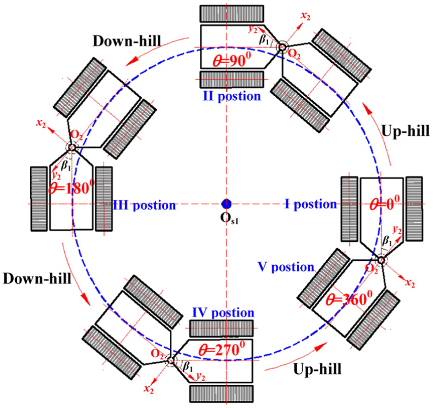
Vehicle movement state during different steering periods.
The simulated results are given as follows.
Variations of the average vertical loads of the inner and outer tracks during slope steering
Figure 12 depicts the following variations of the average vertical loads of the inner and outer tracks during slope steering:
As the azimuth angle θ changes, the variations of the average vertical loads of the inner and outer tracks experience three stages. In the first stage (0° ≤ θ ≤ 90°), the average vertical load of the inner track increases and that of the outer track decreases with an increase in the azimuth angle θ. This phenomenon occurs because the articulated tracked vehicle is uphill driving in this phase, so the pressure center of vehicle gradually moves toward the direction of the inner track under the action of component of gravity of
As the angle of the ramp surface α increases, the average vertical loads of the inner and outer tracks greatly vary. This variation indicates that the angle of the ramp surface α significantly influence the vertical loads of tracks. Due to these uneven distributions of average vertical loads of the inner and outer tracks, the vehicle body may generate a lateral roll-over moment that enables the vehicle body to generate the lateral roll-over during slope steering. Therefore, the angle of the ramp surface α is an important influential factor of the vehicle slope steering stability.
The average vertical load of the inner track is larger than that of the outer track during slope steering. The main reason for this phenomenon is that the pressure center of the articulated tracked vehicle always generates the lateral deviation along the direction of the inner track during slope steering.

Variations of the average vertical loads of the inner and outer tracks during slope steering: (a) variation of the average vertical load of the inner track and (b) variation of the average vertical load of the outer track.
Deviations of the instantaneous rotation centers of the inner and outer tracks affecting frictional resisting forces
Figure 13(a)–(c) indicates that the deviations of the instantaneous rotation centers of the tracks greatly affect the frictional resisting forces of tracks during slope steering.

Deviations of the instantaneous rotation centers of the tracks affecting frictional resisting forces according to the established theoretical model: (a) variation of F xi with different A i and D i , (b) variation of F yi with different A i and D i , and (c) variation of M ri with different A i and D i .
Figure 13(a) illustrates that the deviations of the instantaneous rotation centers of the tracks affect the components of the frictional resisting forces of tracks in the x4-axis direction, F xi . Figure 13(a) also presents that A i greatly affects F xi , and D i slightly affects F xi . When A i is within the range between 0 and 2 m, F xi presents a nonlinear increase. When A i exceeds 2 m, F xi tends to increase slowly.
Figure 13(b) shows that the deviations of the instantaneous rotation centers of the tracks affect the components of the frictional resisting forces of tracks in the y4-axis direction, F yi . Figure 13(b) also shows that A i exerts a slight effect on F yi . However, D i greatly affects F yi . When D i is within the range between 0 and 1.91 m, F yi presents a linear increase. When D i exceeds 1.91 m, F yi tends to increase slowly.
Figure 13(c) shows that the deviations of the instantaneous rotation centers of the tracks affect the frictional resisting moment, M ri . Figure 13(c) also presents that A i slightly affects M ri , and D i exerts a significant effect on F yi . When D i is within the range between 0 and 0.47 m, A i and D i slightly affects M ri . When D i exceeds 0.47 m, M ri tends to increase rapidly and presents a nonlinear increase as A i and D i increase.
Variations of the tractive forces of the inner and outer tracks during slope steering
Figure 14 depicts the following variations of the tractive forces of the inner and outer tracks during slope steering:
As the azimuth angle θ changes, the variations of the tractive forces of the inner and outer tracks present periodical variation. The variations of the tractive forces of the inner and outer tracks experience three stages. In the first stage (0° ≤ θ ≤ 90°), the articulated tracked vehicle is uphill driving; the tractive forces of the inner and outer tracks also increase with an increase in the azimuth angle θ. Meanwhile, the power output form of the inner track gradually transforms from the braking force (i.e. the negative value) to the tractive force (i.e. the positive value). When θ = 90°, the tractive force of the inner track peaks. In the second stage (90° ≤ θ ≤ 270°), the articulated tracked vehicle is downhill driving, so the tractive forces of the inner and outer tracks decrease with an increase in the azimuth angle θ. Meanwhile, the power output form of the inner track gradually transforms from the tractive force to the braking force. When θ = 270°, the braking force of the inner track peaks. In the third stage (270° ≤ θ ≤ 360°), the articulated tracked vehicle again starts uphill driving, so the tractive forces of the inner and outer tracks increase with an increase in the azimuth angle θ. Meanwhile, the power output form of the inner track gradually transforms from the braking force to the tractive force.
As the angle of the ramp surface α increases, the tractive forces of the inner and outer tracks greatly vary. The larger the angle of the ramp surface α, the greater the fluctuation of the variations of the track tractive forces. Therefore, the angle of the ramp surface α greatly influences the power performance of articulated tracked vehicles during slope steering.
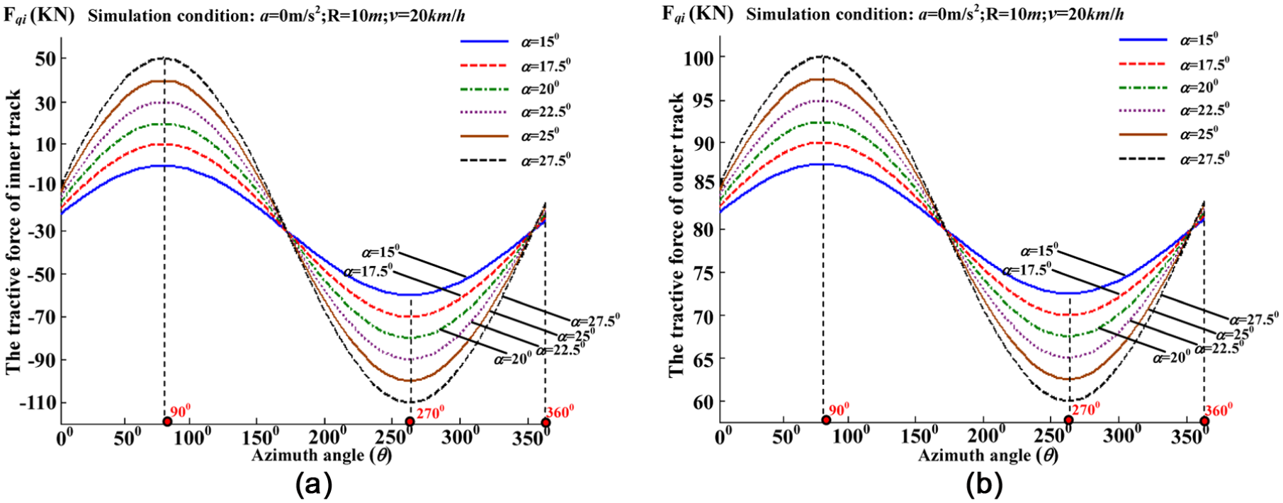
Variations of the tractive forces of the tracks during slope steering: (a) variation of the tractive force of the inner track and (b) variation of the tractive force of the outer track.
Variations of the resisting moments of the inner and outer tracks during slope steering
Figure 15 depicts the variations of the resisting moments of the inner and outer tracks during slope steering. Figure 15 indicates that the variations of the resisting moments of the inner and outer tracks are similar with that of the average vertical loads of the inner and outer tracks. The variations also experience three stages. In the first stage (0° ≤ θ ≤ 90°), the resisting moment of the inner track increases and that of the outer track decreases as the azimuth angle θ increases. In the second stage (90° ≤ θ ≤ 270°), the resisting moment of the inner track decreases and that of the outer track increases as the azimuth angle θ increases. In the third stage (270° ≤ θ ≤ 360°), the resisting moment of the inner track increases and that of the outer track decreases as the azimuth angle θ increases.

Variations of the resisting moments of the tracks during slope steering: (a) variation of the resisting moment of the inner track and (b) variation of the resisting moment of the outer track.
These phenomena occur because track pressure is one of the determinant factors for the track resisting moment. The average vertical load of track directly affects track pressure. Therefore, the variations of the track resisting moments should be consistent with that of the average vertical loads of tracks during slope steering.
Variations of the tractive forces of the inner and outer tracks with various vehicle structural parameters
Figure 16(a)–(f) shows the variations of the tractive forces of the inner and outer tracks with the various structural parameters of the vehicle:
The variation of pressure center height, track length, and track width affects the tractive forces of the inner and outer tracks (Figure 16(a)–(f)). Among these factors, the pressure center height h greatly affects the tractive forces of the inner and outer tracks. The track length L exerts a certain effect on the tractive forces of the inner and outer tracks. The track width b exerts a minimum effect on the tractive forces of the inner and outer tracks.
The pressure center height h greatly affects the tractive forces of the inner and outer tracks. As the azimuth angle θ increases, the variations of the tractive forces of the inner and outer tracks become increasingly intense during slope steering (Figure 16(a) and (b)). When the articulated tracked vehicle is steering on a ramp surface, the variation of pressure center height h greatly affects the vehicle steering performance. Therefore, the variation of the pressure center height h should be given attention during slope steering.
The track length L exerts a certain effect on the tractive forces of the inner and outer tracks (Figure 16(c) and (d)). The tractive forces of the inner and outer tracks also increase with an increase in the track length L. Increasing the length of track L will not be conducive to improve the vehicle slope steering ability.
The track width b exerts a minimum effect on the tractive forces of the inner and outer tracks (Figure 16(e) and (f)). The tractive force of the inner track increases with an increase in the track width b, whereas that of the outer track decreases.
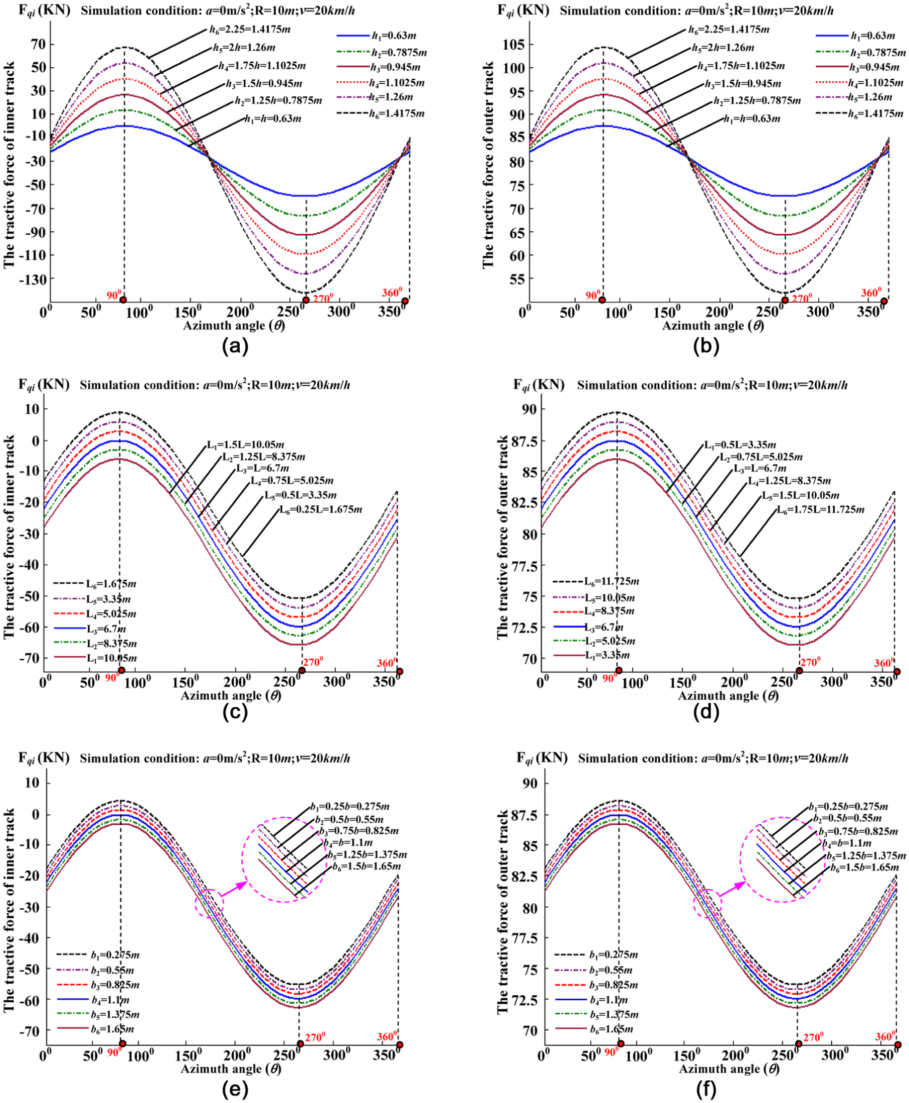
Variations of the tractive forces of the inner and outer tracks under the different pressure center heights h, track lengths L, and track widths b according to the established theoretical model: (a) tractive force of the inner track with different h, (b) tractive force of the outer track with different h, (c) tractive force of the inner track with different L, (d) tractive force of the outer track with different L, (e) tractive force of the inner track with different b, and (f) tractive force of the outer track with different b.
Variations of the tractive forces of the inner and outer tracks with various vehicle accelerations and soil conditions
Figure 17 depicts the variations of the tractive forces of the inner and outer tracks with different vehicle accelerations. Figure 17 shows that the tractive forces of the inner and outer tracks increase as the vehicle acceleration a increases during slope steering. When the articulated tracked vehicle is in an accelerated steering motion state during slope steering, the inner and outer tracks need to generate great tractive forces.

Variations of the tractive forces of the inner and outer tracks under different vehicle accelerations: (a) tractive force of the inner track with different a and (b) tractive force of the outer track with different a.
Figure 18 depicts the variations of the tractive forces of the inner and outer tracks under different soil conditions. The articulated tracked vehicle is steering on the snow where the tractive forces of the inner and outer tracks are largest. When the articulated tracked vehicle is steering on a hard surface, the tractive forces of the inner and outer tracks are the least. Figure 18 illustrates that as the water content of soil increases, the inner and outer tracks must provide larger tractive forces during slope steering.

Variations of the tractive forces of the inner and outer tracks under different soil conditions: (a) tractive force of the inner track under different soil conditions and (b) tractive force of the outer track under different soil conditions.
Comparison between simulation and theoretical results
This study adopts the mechanical-control united simulation model of an articulated tracked vehicle to verify the correctness of the established theoretical model here. The virtual prototype simulation model of the articulated tracked vehicle includes two parts. One part is the mechanical simulation sub-model of the vehicle, as shown Figure 19(a), the joints of the articulated unit, as shown Figure 19(b), and the structural parameters of the vehicle set (Table 3). The road condition is set to a sandy terrain, and its physical parameters set are listed in Table 3. Another part is the control system of steering hydraulic cylinders, as shown Figure 19(c), and the control principles are as follows: (1) when spring A elongates and spring B shortens, the high-pressure oil first enters the reversing valve from the A channel. Then, the high-pressure oil enters the rod port of the left steering hydraulic cylinder and the piston port of the right steering hydraulic cylinder from the Q channel. Consequently, the left and right steering hydraulic cylinders shorten and elongate, respectively. The vehicle finally turns left. (2) On the contrary, when spring A shortens and spring B elongates, the high-pressure oil enters the reversing valve from the B channel. Then, the high-pressure oil enters the piston port of the left steering hydraulic cylinder and the rod port of the right steering hydraulic cylinder from the T channel. Subsequently, the left and right steering hydraulic cylinders elongate and shorten, respectively. The vehicle finally turns right. In the simulation, the parameters of the steering hydraulic cylinders are set as shown in Table 1.

Virtual prototype simulation model of the articulated tracked vehicle: (a) mechanical simulation model of the articulated tracked vehicle, (b) joints of the articulated unit, and (c) control system of the steering hydraulic cylinders based on the AMESim.
Figure 20(a)–(f) illustrates the movement posture of the articulated tracked vehicle during slope steering according to the virtual prototype simulation model. Under the action of the steering hydraulic cylinders, the front vehicle draws the rear vehicle to make the steady steering movement on the ramp surface along its own movement trajectory.

Movement posture of the articulated tracked vehicle during slope steering according to the virtual prototype simulation model: (a) the vehicle is in the initial position, (b) the azimuth angle of vehicle is 0°, (c) the azimuth angle of vehicle is 90°&0x44; (d) the azimuth angle of vehicle is 180°, (e) the azimuth angle of vehicle is 270°&0x44; and (f) the azimuth angle of vehicle is 360°.
Figure 21 depicts the simulated steering trajectory of the articulated tracked vehicle during slope steering. First, the vehicle is driving straightly on the plane. Then, the vehicle is driving straightly on the ramp surface. Finally, the vehicle starts to perform the slope steering motion.

Steering trajectory of vehicle during slope steering according to the virtual prototype simulation model.
The theoretical steering radii are compared with the virtual prototype–simulated steering radii (Figure 22). Figure 22(a)–(c) indicates that the theoretically calculated and simulated results are very close; the relative errors between the theoretically calculated and simulated results are not more than 10%, confirming that the theoretical calculation result is correct.

Theoretical steering radii compared with the virtual prototype–simulated steering radii: (a) the steering radius is 5 m, (b) the steering radius is 10 m, and (c) the steering radius is 15 m.
When β2 is 5° and 35°, the variation curve of the simulated steering moments at the articulated point of O using the virtual prototype simulation model is shown in Figure 23. The variation of the steering moments has four stages. The steering moment is 0 when T is 0–2 s. At this time, the articulated tracked vehicle does not start to turn; the steering moments greatly increase when T is 2–3 s. At this time, the articulated tracked vehicle starts to turn; the steering moments are in a steady state and fluctuate within a stable range when T is 3–5 s; the steering moments gradually decrease to 0 when T is 5–8 s. At this time, the articulated tracked vehicle completes the steering motion.

Variation curve of the simulated steering moments at the articulated point of O according to the virtual prototype simulation model: (a) when the vehicle turns with β2 = 5° and (b) when the vehicle turns with β2 = 35°.
Comparison between experimental and theoretical results
This study proposes an actual slope steering test of the articulated tracked vehicle. In the experimental setup, the experimental vehicle is steady slope steering on different slope surfaces, and the road condition is sandy terrain. The variations of the vehicle velocities and the steering angles are controlled in the 0–37 km/h and −35° ± 35° ranges, respectively. The engine speed is required to maintain a stable working state during the slope steering test. The measured data of the output torques of the inner and outer wheel-side decelerators, steering angles of β2, oil pressures of the steering hydraulic cylinders, vehicle velocities, azimuth angle θ, and steering trajectories are recorded during the process. The measured system of the slope steering test for the articulated tracked vehicle is shown in Figure 24. A non-contact digital torque instrument called PH487 is used in the test to measure the torques by installing it on the shafts of the inner and outer wheel-side decelerators. The oil pressures of the steering hydraulic cylinders are measured by placing the oil pressure transducer (i.e. PT500) into the portals of the oil pumps of the steering hydraulic cylinders. The vehicle velocities, azimuth angle θ, and steering trajectories are measured by the vehicle Global Positioning System (GPS). This GPS comprises basic and mobile station subsystems. In the slope steering test, the basic station subsystem is fixed on the ground, and the first radio set is used to send a signal, and the mobile station is fixed on the front vehicle and then subsequently moves, and the second radio set is fixed on the top of the front vehicle to accept the signal from the basic station.
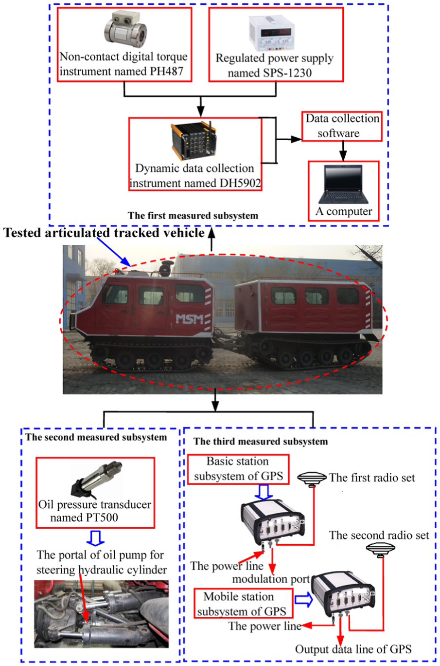
Measured system of the slope steering test for the articulated tracked vehicle.
Figure 25 presents the measured data of the oil pressures for the steering hydraulic cylinders during steering. Consistent with the simulated results, the variation of the actual measured oil pressures also experiences three stages.

Measured data of oil pressure for the steering hydraulic cylinder in the actual slope steering test.
Table 5 shows the theoretical, simulated, and experimental steering moment results. The relative errors between the simulated and experimental results are not more than 19.8%, and those between the theoretical and experimental results are not more than 9.2%. The simulated and experimental results closely agree with the theoretical results. The correctness of the theoretical model is thus verified.
Theoretical steering moments compared with the virtual prototype–simulated and experimental steering moments.
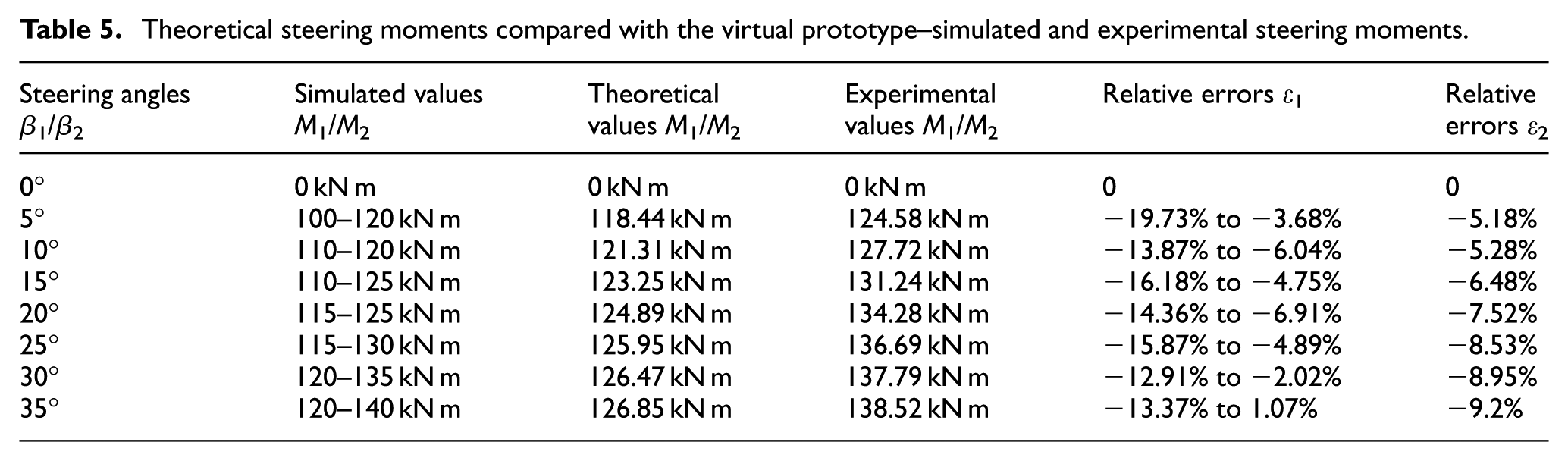
In addition, the relative errors between the simulated and experimental results are relatively large. The simulated precision is reduced because the virtual prototype simulation model is assumed to have the rigid body of the track and road surface. The track and road surface do not generate deformation in the simulation process. The tension forces of the tracks are also not considered to affect steering performance in the simulation model. However, the track and road surface can generate deformation during actual steering. The tension forces of the tracks may also affect steering performance. Therefore, the simulated results present a certain error compared with the experimental results.
The tested tractive forces of the inner and outer tracks are compared to the theoretical calculated results shown in Figure 26. Figure 26(a)–(d) indicates that the variation trends of the tested and calculated tractive forces for the inner and outer tracks are consistent. The tested and theoretically calculated results of the tractive forces for the inner and outer tracks are very close, thus verifying the precision of the theoretical model.
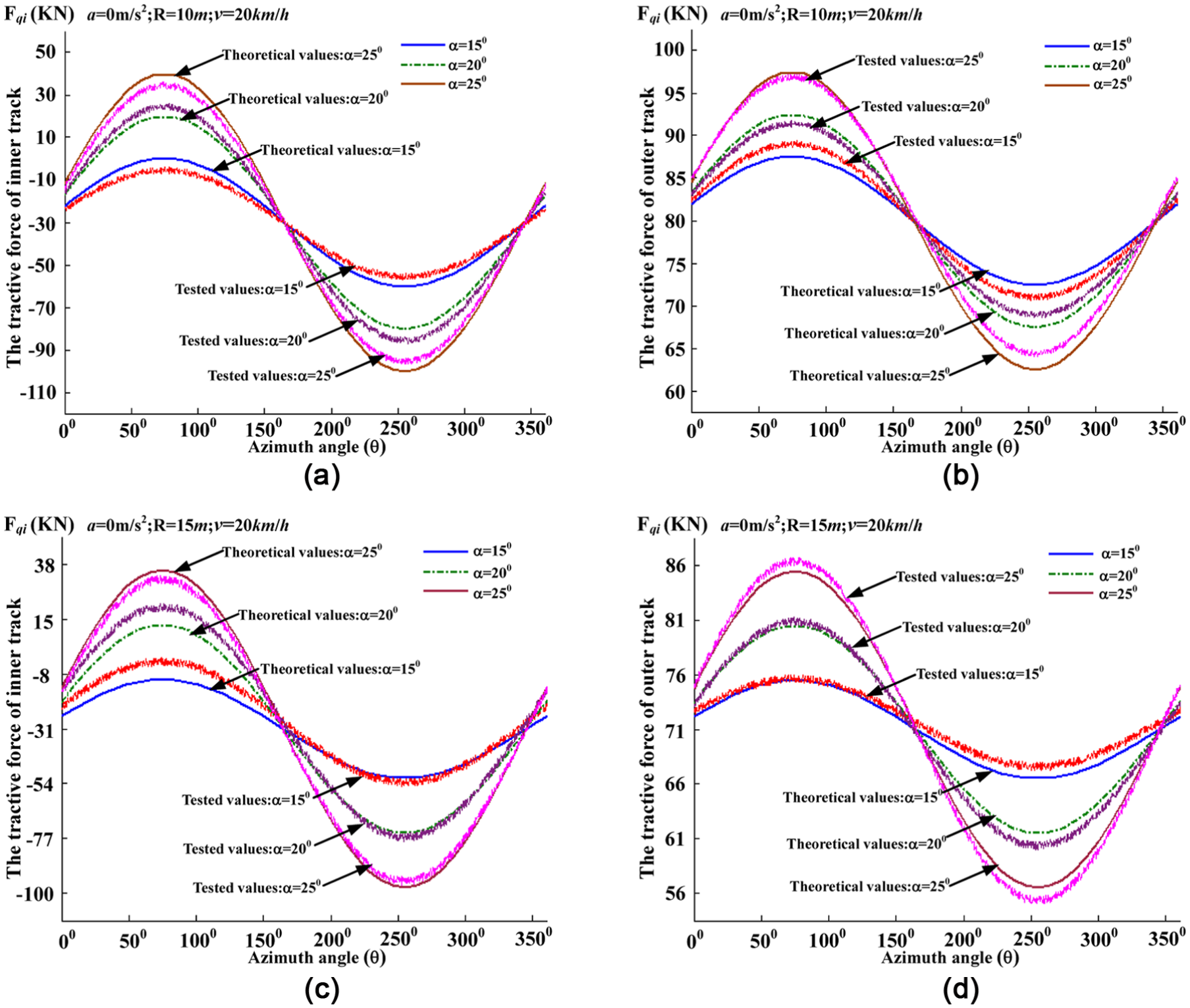
Simulated tractive forces of the inner and outer tracks compared with the theoretical calculated results: (a) tractive force of inner track when R = 10 m, (b) tractive force of outer track when R = 10 m, (c) tractive force of inner track when R = 15 m, and (d) tractive force of outer track when R = 15 m.
Conclusion
This study proposes a novel dynamic modeling method to evaluate the steering performance of articulated tracked vehicles on the ramp. The steering performance of a specific articulated tracked vehicle on the ramp surface is discussed in detail using an established theoretical model. The virtual prototype simulation and actual slope steering test on the articulated tracked vehicle demonstrate a close agreement with the theoretical results. The proposed model can provide a theoretical method for predicting and evaluating the steering performance of articulated tracked vehicles on the ramp.
The results show that the angle of ramp surface α, the pressure center height h, the track length L, and the track width b affect the steering performance of articulated tracked vehicles. However, among these factors, α and h exert greater influence on the steering performance than L and b. Therefore, the changing situations of α and h should be focused on when analyzing vehicle slope steering performance.
Footnotes
Appendix 1
Appendix 2
Appendix 3
Appendix 4
Appendix 5
Appendix 6
Appendix 7
Academic Editor: Fakher Chaari
Declaration of conflicting interests
The author(s) declared no potential conflicts of interest with respect to the research, authorship, and/or publication of this article.
Funding
The author(s) disclosed receipt of the following financial support for the research, authorship, and/or publication of this article: This research was financially supported by the National Natural Science Foundation of China (No. 51375202) and National Science and Technology Major Projects Funded Item (No. 2009DFR80010).