Sage Journals: Discover world-class research

Abstract

The automation level has been improved rapidly with the introduction of large-scale measurement technologies, such as indoor global positioning system, into the production process among the fields of car, ship, and aerospace due to their excellent measurement characteristics. In fact, the objects are usually in motion during the real measurement process; however, the dynamic measurement characteristics of indoor global positioning system are much limited and still in exploration. In this research, we focused on the dynamic tracking performance of indoor global positioning system and then successfully built a mathematical model based on its measurement principles. We first built single and double station system models with the consideration of measurement objects’ movement. Using MATLAB simulation, we realized the dynamic measurement characteristics of indoor global positioning system. In the real measurement process, the experimental results also support the mathematical model that we built, which proves a great success in dynamic measurement characteristics. We envision that this dynamic tracking performance of indoor global positioning system would shed light on the dynamic measurement of a motion object and therefore make contribution to the automation production.

Keywords

iGPS dynamic measurement mathematical model experimental study

Introduction

With the rapid development of modern science and technology, manufacturing process has been greatly improved and become with the features of informatization, automatization, intelligentialization, and integration.^1,2 In assembly process of manufacturing industry, people often use some new technologies to improve the automatization level.² It is widely considered that the quality, precision, and efficiency of the measurement technology are significantly important in the automation assembly process since they determine the success of the assembly process.³ As a traditional and popular large-scale measurement technology, laser tracker is widely used in the assembly process of manufacturing industry,^4,5 yet the small measuring range and single point measuring of laser tracker still limit its industrial application.

As a new large-scale measurement technology, indoor global positioning system (iGPS) provides a novel way to realize automation assembly due to its high precision, high efficiency, high reliability, and multi-point tracking ability at the same time.^6,7 It has been demonstrated that iGPS is used in various automation assembly processes among aerospace, automotive, and ship-building structures (e.g. the jigless assembly of aircraft components and the positioning of automatic robots).⁸ It is also reported that the iGPS in some cases presented better results than a laser tracker.⁹ In the past decades, lots of researches on static measurement characteristics of iGPS have been conducted. For instance, DA Maisano et al.¹⁰ clearly stated that measurement accuracy of iGPS could improve if the number of transmitters increases, while the change will not be too much if the number of transmitters is four or more. In 2009, JE Muelaner et al.¹¹ discussed the uncertainty of angle measurement for a single transmitter and gave out the relationship diagram. It was proved by R Schmitt et al.¹² that the layout of transmitters could significantly influence its measurement accuracy and the C Type Layout presented better precision. In fact, the objects are normally in motion during the assembly process which causes measurement deviation of iGPS based on its operational principles. For these applications, the objects need to be dynamically tracked in order to monitor the whole process. Most recently, some scholars have started to investigate the accuracy in iGPS dynamic measurement. For example, Claudia Depenthal¹³ claimed that the dynamic measurement accuracy of iGPS would decrease if the measurement object is in rotational movement. Zheng Wang et al.⁹ considered that the velocity direction of the measurement object could influence the increment direction of deviation. Unfortunately, there is little work on the qualitative relationship between the measurement deviation and the object’s velocity, and the dynamic tracking performance of iGPS system still remains to be a big challenge.

In this article, we focused on the dynamic tracking performance of iGPS in automation production process through theoretical simulation and experimental study. The emphasis of this article lied in the estimation of dynamic measurement accuracy by exploring the quantitative relationship between the object’s velocity and the measurement angles relative to transmitters. First, we proposed a single station system model to compensate the angle deviation when the object is in motion. Then, we used the angles’ information relative to two transmitters to obtain the object’s position by building a double station system model. Most importantly, the experimental study demonstrated that the deviation has a linear relationship with the object’s velocity, which was in accordance with the MATLAB simulation, and both of the theoretical simulation and experimental study results indicated the great success of iGPS applied in dynamic measurements. We consider that the results of our reported work will improve the measurement accuracy of iGPS for tracking dynamic objects and guide the direction of practical industrial production when high precision of iGPS is needed for assembly process.

Mathematics model

An iGPS system typically consists of two or more transmitters, a control center, a number of wired/wireless sensors, and a scale bar. During the measurement process, transmitters, which operate as reference points, continually generate three signals: an infrared light-emitting diode (LED) strobe and two infrared laser fanned beams that rotate in the head of the transmitter. Each transmitter presents two measurement values to each sensor: the horizontal (azimuth, φ) and the vertical angles (elevation, θ), as shown in Figure 1(a). The position calculation engine (PCE) can calculate these measurement values related to transmitters trough pulsing signals, which are gained from the sensor being placed on the surface of the object. If the sensor is located in the line sight of two or more transmitters, whose coordinate locations have been solved before starting measuring, and the position of sensor can be calculated based on the measurement principle of triangulation, as shown in Figure 1(b).

Figure 1.

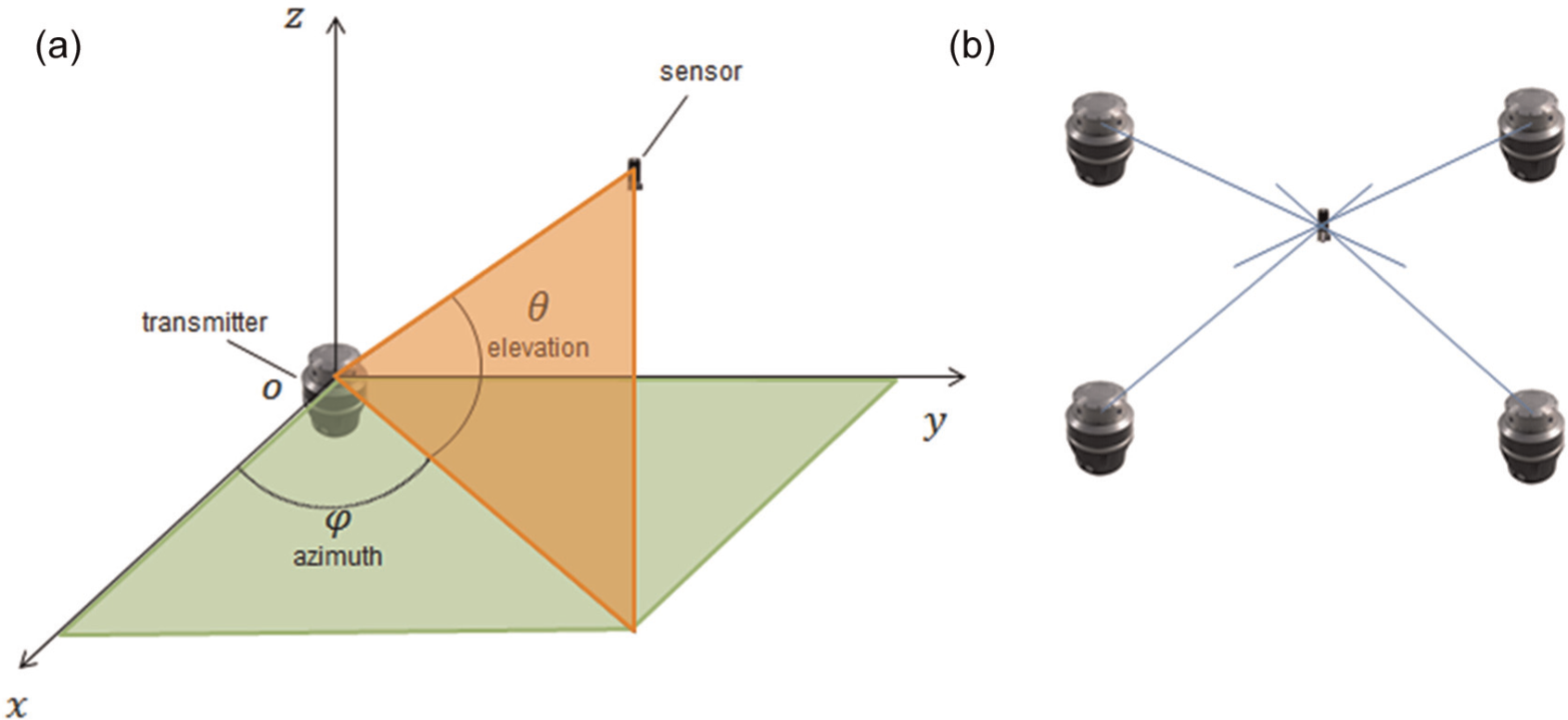
Measurement principle of iGPS. (a) The transmitter presents two measurement values: the azimuth angle (φ) and elevation angle (θ). When the coordinate system of the transmitter is fixed, the position of sensor can be located in a line related to the transmitter based on these two angles. (b) If two or more transmitters are placed in the measuring volume, the accurate position of sensor is at the line intersection.

Considering that two fanned lasers sweeping through the measuring volume with a predetermined speed at the beginning of the measurement process and the strobe illuminating the volume, a sensor that is placed in the volume can receive two kinds of optical signals (flat light and synchronous light) and convert these optical signals into pulsing signals. During a measurement cycle, a sensor creates a pulsing signal to record the beginning moment (t ₀) on receiving a synchronous signal and create two timing pulsing signals to record the time (t ₁ and t ₂) when it receives two flat signals. Based on these pulsing signals and the postures of two flat planes, the azimuth angle and elevation angle of a sensor related to a transmitter can be calculated as presented in Figure 2.

Figure 2.

Two infrared laser fanned beams and an infrared LED strobe of a transmitter. (a) A transmitter continually operates an infrared LED strobe and two infrared laser fanned beams during its working process. The angle between fan 1 (L₁) and fan 2 (L₂) is about φ_off in the horizontal plane of the transmitter. (b) During a measurement cycle, a sensor receives three signals from each transmitter. When it receives a signal of the infrared LED strobe, it creates a pulse to record the time of t ₀. The time of t ₁ and t ₂ is to record the moment when the sensor receives the signals of fan 1 and fan 2.

Since these two infrared laser fanned beams do not reach the sensor simultaneously, time delay will cause measurement deviation if the sensor which is set as a measurement point is in motion. In order to obtain the accurate position, a single station system model is proposed to compensate the deviation of two measurement values related to each transmitter. When a transmitter launches a synchronous signal, the intersecting line of the light plane and transmitter’s horizontal plane is defined as x-axis, the rotation axis is defined as z axis, and the y axis can be determined by the right-hand rule. This measurement process can be seen in Figure 3 for a measurement cycle.

Figure 3.

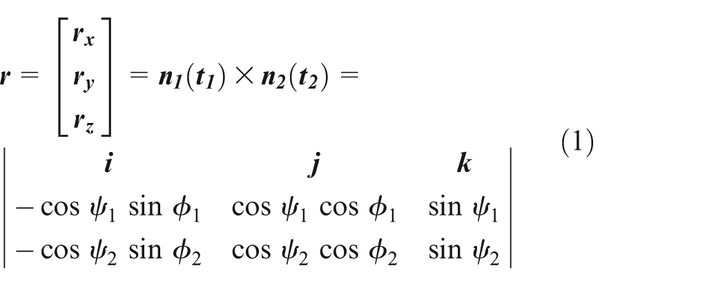
Measurement process for a single station. (a) At the beginning moment of t ₀, the normals to the planes of fan 1 and fan 2 are n ₁(t ₀) and n ₂(t ₀). (b) Through t ₁, fan 1 has rotated φ ₁ about the z axis and its normal turns n ₁(t ₁). (c) Then the normal to fan 2 becomes n ₂(t ₂) at t ₂. (d) The point lies on the first fan at t ₁ and the second fan at t ₂, and its direction vector related to the origin coordinate can be calculated through cross product.

If we bypass its motion, the direction vector of the measurement point can be given by equation (1) as follows

\begin{matrix} r = [\begin{matrix} r_{x} \\ r_{y} \\ r_{z} \end{matrix}] = n_{1} (t_{1}) \times n_{2} (t_{2}) = \\ | \begin{matrix} i j k \\ - \cos ψ_{1} \sin ϕ_{1} \cos ψ_{1} \cos ϕ_{1} \sin ψ_{1} \\ - \cos ψ_{2} \sin ϕ_{2} \cos ψ_{2} \cos ϕ_{2} \sin ψ_{2} \end{matrix} | \end{matrix}

(1)

where $ϕ_{1}$ and $ϕ_{2}$ are the angles between the fan and the x-axis when the point receives the signals of fan 1 and fan 2, and ψ ₁ or ψ ₂ is the intersection angle which is between the fan and the z-axis. However, the point is often in motion during the measurement process. In this situation, when the point receives the signal of two infrared laser fanned beams, it is not at the original position of t ₀ which is needed to be measured. Thus, the values of $ϕ_{1}$ and $ϕ_{2}$ should be compensated considering the motion of the point. If the point that is far away from the original point in coordinate system (R) is in motion of the velocity (v), the accurate rotation angle of fan 1 aligned with the x-axis can be calculated by

ϕ_{1} = ω \cdot (t_{1} - t_{0}) - Δ ϕ

(2)

where $Δ ϕ$ is the compensation angle when the velocity of the point is considered and can be expressed as

Δ ϕ = ω_{m} \cdot (t_{1} - t_{0})

(3)

where ω _m is the angular velocity of the measurement point aligned with the rotation axis of the transmitter, which is positive value when its rotation direction is the same as that of the transmitter. Since the product of the velocity (v) and time (t) is much less than R, equation (3) can be transformed into

Δ ϕ = ω_{m} \cdot (t_{1} - t_{0}) = α \frac{v}{R} \cdot (t_{1} - t_{0})

(4)

where α is the coefficient, which is determined by the angle between the normal to fan 1 and the direction of velocity. And the values of $ϕ_{1}$ and $ϕ_{2}$ can be given by

{\begin{matrix} ϕ_{1} = ω \cdot (t_{1} - t_{0}) - α \frac{v}{R} \cdot (t_{1} - t_{0}) \\ ϕ_{2} = ω \cdot (t_{2} - t_{0}) - β \frac{v}{R} \cdot (t_{2} - t_{0}) - ϕ_{off} \end{matrix}

(5)

where β is the coefficient, which is determined by the angle between the normal to fan 2 and the direction of velocity, and $ϕ_{off}$ is the angle between fan 1 and fan 2 in the horizontal plane of the transmitter.

Finally, if we consider the influence of the velocity, the azimuth angle (φ) and elevation angle (θ) of the measurement point related to the transmitter can be calculated by

\begin{matrix} φ = - \frac{v}{R} \cdot \frac{(α (t_{1} - t_{0}) + β (t_{2} - t_{0}))}{2} \\ + \frac{ω \cdot ((t_{1} - t_{0}) + (t_{2} - t_{0})) - ϕ_{off}}{2} \end{matrix}

(6)

\begin{matrix} θ = \arctan \\ (\frac{2 \sin (- \frac{v}{R} \cdot \frac{(α (t_{1} - t_{0}) + β (t_{2} - t_{0}))}{4} + \frac{ω \cdot ((t_{1} - t_{0}) + (t_{2} - t_{0})) - ϕ_{off}}{4})}{\tan ψ}) \end{matrix}

(7)

From discussion above, we can see that the single station system model can obtain the point’s relatively position to one transmitter; however, the accurate position must be determined by at least two transmitters. Therefore, we proposed a double station system model which has compensated angle deviation to calculate the accurate position of the point in the following section.

For the double station system model, there are two transmitters (A and B) in the measuring volume, and the position of M can be calculated accurately because each coordinate value contains two components. For example, the x-axis value consists of x ₁ and x ₂. As presented in Figure 4, the distance between A and B is 2d in the horizontal direction, 2l in the y-axis direction, and 2h in the vertical direction. Thus, the components of the coordinate value of M can be given by

{\begin{matrix} x_{1} = \frac{2 (l - d \tan φ_{B})}{\tan φ_{A} - \tan φ_{B}} - d \\ x_{2} = \frac{2 (l - d \tan φ_{A})}{\tan φ_{A} - \tan φ_{B}} + d \\ y_{1} = \frac{2 (l - d \tan φ_{B})}{1 - \cot φ_{A} \tan φ_{B}} - l \\ y_{2} = \frac{2 (l - d \tan φ_{A})}{\cot φ_{B} \tan φ_{A} - 1} + l \\ z_{1} = \frac{2 (l - d \tan φ_{B})}{\cos θ_{A} (\sin φ_{A} - \cos φ_{A} \tan φ_{B})} - h \\ z_{2} = \frac{2 (l - d \tan φ_{A})}{\cos θ_{B} (\cos φ_{B} \tan φ_{A} - \sin φ_{B})} + h \end{matrix}

(8)

Figure 4.

General double station system model. In the double station system model, there are two transmitters (A and B) in the measuring volume, and the position of M can be calculated accurately based on this model.

where φ_A and φ_B are the azimuth angles related to transmitters A and B, and θ_A and θ_B are the elevation angles, which can be gained from equations (6) and (7). As the start time of these two transmitters are different, special processing should be carried out when calculating the azimuth angle (φ_B ) and elevation angle (θ_B ) in the single station system of transmitter B, whose infrared LED strobe is supposed to sweep the point later. In this situation, the values of $ϕ_{1}$ and $ϕ_{2}$ can be described as

{\begin{matrix} ϕ_{1} = ω \cdot (t_{1} - t_{0}) - α \frac{v}{R} \cdot ((t_{1} - t_{0}) + Δ t) \\ ϕ_{2} = ω \cdot (t_{2} - t_{0}) - β \frac{v}{R} \cdot ((t_{2} - t_{0}) + Δ t) - ϕ_{off} \end{matrix}

where Δt is the time interval between the start time of these two transmitters.

From equation (8), the position of M can be calculated by

x = \frac{x_{1} + x_{2}}{2}, y = \frac{y_{1} + y_{2}}{2}, z = \frac{z_{1} + z_{2}}{2}

(9)

During the measurement process, the position of M is considered to be (x ₀, y ₀, z ₀)^T when it is static. However, if the velocity of M is v, the position of M is (x, y, z)^T under the same measurement condition at this moment. Thus, the deviation of the coordinate values can be given by

ε = ‖ {(x, y, z)}^{T} - {(x_{0}, y_{0}, z_{0})}^{T} ‖_{2}

(10)

To be noted, a sensor, which represents the measurement point, can receive signals from several transmitters in the measuring volume, and the system will calculate its position based on the signals from two random transmitters. In this consideration, the position of M may have several values. The system will combine those values together and obtain its final coordinate value.

Results and discussion

To investigate the dynamic tracking performance of iGPS, we first give the relationship between the dynamic measurement accuracy of iGPS and velocity of the measurement point using MATLAB simulation. For the working conditions of a single station system model, the point which is in motion with the velocity of v is R far away from the original point of one transmitter coordinated system, and the results are presented in Figure 5. Worth noting is that in the process of simulation, R is equal to 3 m, while v varies from −200 to 200 mm/s, t ₀ is equal to 0 s, t ₁ is equal to 0.005 s, t ₂ is equal to 0.009 s, and ω is equal to 89.6π.

Figure 5.

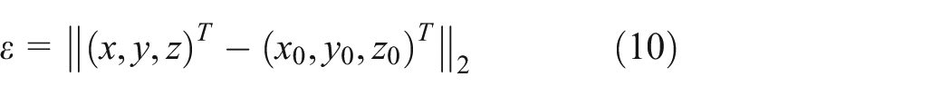
Simulation results of a single station system model. (a) The azimuth angle (φ) in the single station system model is in a linear relationship with the velocity of the point, while its increment direction is in the opposite direction of the velocity. (b) The elevation angle (θ) is in a linearly negative correlation relationship with velocity.

The static values of the azimuth angle (φ) and elevation angle (θ) are the standard data which need to be obtained when the velocity of the point is 0 mm/s. However, these measurement values will change if the point is in motion, as illustrated in Figure 5(a). The azimuth angle is in a linear relationship with the velocity of the point in the range of velocity varying from −200 to 200 mm/s. If the velocity is −200 mm/s, the azimuth angle is 67.923°, and its value will decrease to 67.870° when the velocity accelerates to 200 mm/s. As illustrated in Figure 5(b), the relationship between the elevation angle and the velocity of the point presents to be similar with the relationship of azimuth angle (φ), which is shown in Figure 5(a). When the velocity of the point varies from −200 to 200 mm/s, the elevation angle decreases proportionally with the minimum value of −20.922° and the maximum value of −20.900°. From equations (6) and (7), we consider that if the linear relationship in the single station system is obtained, the deviation of azimuth angle and elevation angle can be compensated.

It is noted that if there are several transmitters in the measuring volume and their measurement values are compensated, the accurate position of the point can be calculated by two arbitrary transmitters through the triangulation principle. Thus, in the following section, we built a double station system model to solve this problem with the help of MATLAB simulation. It is assumed that the distance between transmitters A and B is 2329.3804 mm in horizontal direction, 3494.0941 mm in the y-axis direction, and 2852.0811 mm in vertical direction. The position of A is (−1164.6902, 1747.04705, and −1426.04055) and the position of B is (1164.6902, −1747.04705, 1426.04055), and the result is summarized in Figure 6. For the transmitter A, fan 1 sweeps the point after (t ₁–t ₀), and fan 2 sweeps the same point after (t ₂–t ₀), where t ₀ is equal to 0 s, t ₁ is equal to 0.004 s, t ₂ is equal to 0.0086 s, and f ₁ is equal to 44.8 Hz. For the transmitter B, fan 1 sweeps the point after (t ₄–t ₃), and fan 2 sweeps the same point after (t ₅–t ₃), where t ₃ is equal to 0.0056 s, t ₄ is equal to 0.0088 s, t ₅ is equal to 0.0116 s, and f ₂ is equal to 43.0 Hz. In the measuring volume, the velocity of the measurement point varies from −200 to 200 mm/s.

Figure 6.

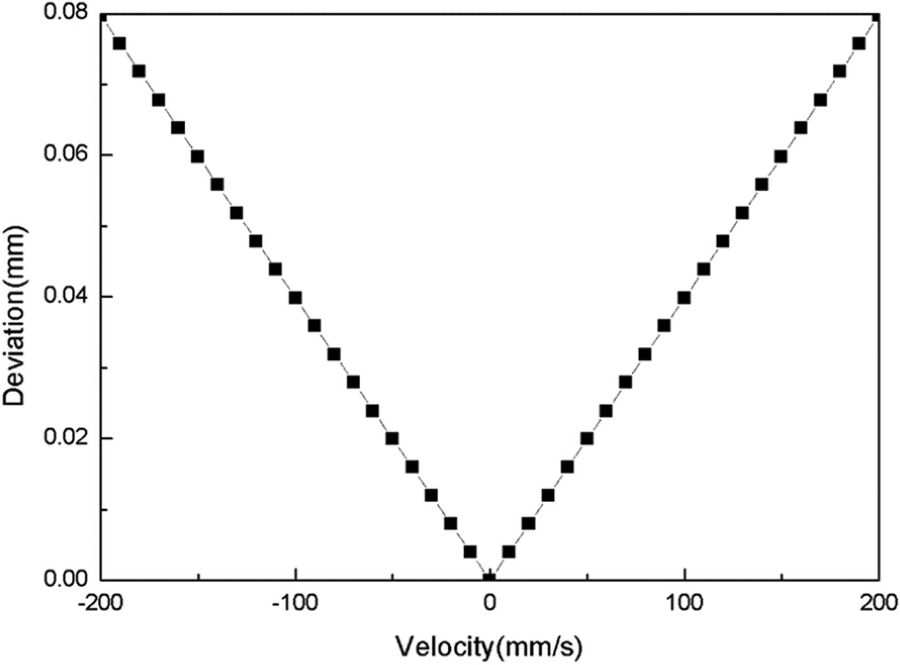
Relationship between the velocity and deviation in the double station system model. When the velocity of the point is 0 mm/s, the deviation is 0 mm without considering the influence of other factors. The deviation is in a linear relationship with the velocity, and it increases if the absolute value of velocity rises in the MATLAB simulation.

As illustrated in Figure 6, the deviation in the double station system model is in a linear relationship with the point velocity in the range from −200 to 0 mm/s or from 0 to 200 mm/s. The deviation is considered to be 0 mm when the velocity is 0 mm/s without considering influence of other factors, and the deviation will enhance with the increase in velocity absolute value. Moreover, while the velocity varies from −200 to 200 mm/s, the maximum value of deviation reaches 0.08 mm.

We also conducted an experiment to verify the double station system model, as presented in Figure 7. During the experimental process, the min-vector bar which was set on the slider of the linear membrane group moved with a set velocity varying from −162.5 to 162.5 mm/s, while the two transmitters (Figure 7(a)) were used to measure the position of the min-vector bar. The distance of the slider moving in a second was measured by iGPS, and the standard distance was given by the control system of linear membrane group. Then we compared the distance with the standard value and obtained the deviation. The experimental results proved a positive correlation between the deviation and the min-vector bar’s velocity as shown in Figure 7(b), which was in accordance with the double station system model that we established in section “Mathematics model.” Therefore, if the parameters, including the object’s velocity, time signals, and rotating frequencies, are known, the deviation of each position in the iGPS measuring volume can be theoretically compensated.

Figure 7.

Experimental results of dynamic tracking performance of iGPS. (a) The iGPS sensor and transmitter used in our experiments. (b) Experimental results of the double station system model. The black dots are the experimental results done by two transmitters and the linear membrane group, and the blue line is the theoretical calculation. It is shown that the relationship between the deviation and the velocity is in a positive correlation, which verifies the established double station system model.

Conclusion

As an alternative solution for describing dynamic tracking performance of iGPS, we propose a method to compensate the measurement results of iGPS. We first built a set of mathematical models including single and double station system models. It has been verified that the relationship between measurement angles and velocity of the object is in linear correlation when the velocity varies from −200 to 200 mm/s in the single station system model with the help of MATLAB simulation. Based on the single station system model, the measurement values of transmitters in the measuring volume can be compensated. Then we chose two random transmitters to calculate the coordinate deviation of the object in double station system model. And we proved that the deviation is in a linear relationship with the velocity of the object in the range from −200 to 0 mm/s or from 0 to 200 mm/s. Therefore, the coordinate of each point in the measuring volume can be theoretically compensated based on the double station system model during the measurement process of iGPS. We also performed an experiment to evaluate the reasonability of our theoretical study, and the results indicated a positive correlation between the deviation and the velocity, which provided additional support to the mathematical model that we built. We consider that this work we reported would improve the measurement accuracy of iGPS for tracking dynamic objects and shed light on the industrial application of iGPS in automation assembly.

Footnotes

Academic Editor: Elsa de Sa Caetano

Declaration of conflicting interests

The author(s) declared no potential conflicts of interest with respect to the research, authorship, and/or publication of this article.

Funding

This work was supported by the Fund of National Engineering and Research Center for Commercial Aircraft Manufacturing (SAMC13-JS-15-027).

References

Chen

Fang

. Intelligentized technologies for welding manufacturing. In: Kiet Tieu

Zhu

(eds) Materials science forum (Vols. 773–774). Switzerland: Trans Tech Publications Ltd, 2013, pp. 725–731.

Zhou

. Digitalization and intelligentization of manufacturing industry. Adv Manuf 2013; 1: 1–7.

Mei

Maropoulos

. Review of the application of flexible, measurement-assisted assembly technology in aircraft manufacturing. Proc IMechE, Part B: J Engineering Manufacture. Epub ahead of print 7 February 2014. DOI: 10.1177/0954405413517387.

Liu

Xie

. Laser tracker based robotic assembly system for large scale peg-hole parts. In: 2014 IEEE 4th annual international conference on cyber technology in automation, control, and intelligent systems (CYBER), Hong Kong, 4–7 June 2014, pp.574–578. New York: IEEE.

Zhang

Shi

. A dimensional measurement method based on a laser tracker for a crane assembly. Laser Eng 2013; 26: 91–101.

Norman

Schönberg

Gorlach

. Validation of iGPS as an external measurement system for cooperative robot positioning. Int J Adv Manuf Tech 2013; 64: 427–446.

Muelaner

Wang

Martin

. Verification of the indoor GPS system, by comparison with calibrated coordinates and by angular reference. J Intell Manuf 2012; 23: 2323–2331.

Sharke

. Measuring across space and time. Mech Eng 2003; 125: 48–49.

Wang

Mastrogiacomo

Franceschini

. Experimental comparison of dynamic tracking performance of iGPS and laser tracker. Int J Adv Manuf Tech 2011; 56: 205–213.

10.

Maisano

Jamshidi

Franceschini

. A comparison of two distributed large-volume measurement systems: the mobile spatial co-ordinate measuring system and the indoor global positioning system. Proc IMechE, Part B: J Engineering Manufacture 2009; 223: 511–521.

11.

Muelaner

Wang

Jamshidi

. Study of the uncertainty of angle measurement for a rotary-laser automatic theodolite (R-LAT). Proc IMechE, Part B: J Engineering Manufacture 2009; 223: 217–229.

12.

Schmitt

Nisch

Demeester

. Performance evaluation of iGPS for industrial applications. In: 2010 international conference on indoor positioning and indoor navigation (IPIN), Zürich, 15–17 September 2010, pp.1–8. New York: IEEE.

13.

Depenthal

. Path tracking with IGPS. In: 2010 international conference on indoor positioning and indoor navigation (IPIN), Zürich, 15–17 September 2010, pp.1–6. New York: IEEE.

Dynamic tracking performance of indoor global positioning system: An experimental and theoretical study

Abstract

Keywords

Introduction

Mathematics model

Results and discussion

Conclusion

Footnotes

Declaration of conflicting interests

Funding

References