Sage Journals: Discover world-class research

Abstract

As a hydro-mechanical servo system, the whole performance of the two-dimensional proportional valve with magnetic coupling (2D-MC-PV) highly depend on certain structural parameters. To tradeoff good static/dynamic characteristics, good working stability and low leakage pilot stage, a multi-objective optimization is inevitable for preliminary design stage. Therefore, this paper proposes a multi-objective optimization method based on AMESim and Matlab/Simulink co-simulation model, which optimizes key structural parameters by adjusting weight coefficients (balancing static, dynamic, and pilot leakage performance). Considering that magnetic coupling (MC) is the key component for 2D-MC-PV to realize spool position feedback and translational motion conversion, the analytical equation of MC is derived based on the Coulomb’s law and the law of equivalent magnetic charge, and the Monte Carlo method is used to calculate. Finally, the prototype of 2D-MC-PV is designed and manufactured, and a special experimental platform is built to test the static/dynamic characteristics. The experimental results show that 2D-MC-PV has good working stability: under working pressure of 20 MPa, the maximum no-load flow rate is 108.8 L/min with the hysteresis of 3.36%, and the amplitude and phase frequency width is 27.8 and 36.6 Hz. It shows that the multi-objective optimization method proposed in this paper can be used as an optimization method for 2D-MC-PV.

Keywords

Multi-objective optimization co-simulation proportional valve two-dimensional valve magnetic force static/dynamic characteristics

Introduction

Since the 1940s, electro-hydraulic servo control technology has been widely used in key strategic industrial fields such as aerospace, military weapons, and metallurgical equipment.^1–3 The reason is that the electro-hydraulic servo control technology has the advantages of high dynamic response and high control precision.⁴ However, as a key component in the e electro-hydraulic servo technology, the servo valve requires high oil quality and machining accuracy.^5,6 The above reasons make electro-hydraulic servo technology unable to meet the needs of the civilian field. In order to solve the problem of servo valve, proportional valve came into being.^7–9 Compared with the electro-hydraulic servo valve, the electro-hydraulic proportional valve has strong robustness and low cost. Therefore, electro-hydraulic proportional valves have been widely used in many civil fields.^10–14

As the proportional valve is an important development direction of the electro-hydraulic servo control technology, researchers are constantly exploring the proportional valve’s structural innovation.^9,15–19 However, the independence of the pilot stage and the power stage makes it difficult to improve the power-to-weight ratio of the proportional valve.^20,21 Ruan et al.^22–24 proposed a two-dimensional proportional valve, which innovatively integrates the pilot stage and the power stage on the spool. Ruan’s^25–27 team tried a variety of structures, but was trapped by the nature of the inevitable contact of mechanical transmission. To eliminate the friction, wear, and fit clearance, Bin et al.²⁸ proposed a two-dimensional proportional valve with magnetic coupling (2D-MC-PV). The magnetic coupling (MC) is the key component of 2D-MC-PV. It converts the linear displacement of L-EMC into a rotation angle through non-contact magnetic force (no friction), and completes the position feedback function. The experimental results show that 2D-MC-PV has good static/dynamic characteristics and is suitable for civil applications.²⁸

At present, 2D-MC-PV has only reached the stage of principle realization, and its performance still has a lot of room for improvement. As a hydro-mechanical servo system, the whole performance of the 2D-MC-PV highly depend on certain structural parameters. To tradeoff good static/dynamic characteristics, good working stability, and low leakage pilot stage, a multi-objective optimization is inevitable for preliminary design stage. The swarm intelligent algorithms have strong robustness, strong search ability, and is easy to combine with other algorithms to improve algorithm performance.^29–31 Therefore, the swarm intelligent algorithms are suitable as a multi-objective optimization algorithm for 2D-MC-PV. Swarm intelligent algorithms mainly include ant Glowworm Swarm Optimization (GSO), Brain Storm Optimization (BSO,) and Particle Swarm Optimization (PSO).³² Among them, PSO has simple evolution process, fast operation speed, and strong global search ability, which is suitable for solving high-dimensional and multi-objective optimization problems.^33–35 Therefore, PSO in the swarm intelligent algorithms is specifically selected as the multiobjective optimization algorithm of 2D-MC-PV. In addition, PSO needs to establish a mathematical model for calculating the fitness value as a fitness function. AMESim software can provide a comprehensive simulation environment of hydraulic system for the mathematical model (fitness function) of 2DMC-PV, and provides interfaces with software such as Matlab and ADAMS. Therefore, this paper proposes a multi-objective optimization method based on AMESim and Matlab/Simulink co-simulation model, which optimizes key structural parameters by adjusting weight coefficients (balancing static, dynamic, and pilot leakage performance). The PSO algorithm is performed with a Matlab script. And Simulink serves as the interface between Matlab scripts and AMESim software.

MC is the key component of 2D-MC-PV to realize spool position feedback and translational motion conversion. In order to design MC that meets the working requirements of 2D-MC-PV, it is necessary to derive its analytical equation. MC realizes its function through the magnetic repulsion generated between the permanent magnets, which is essentially the result of the interaction of countless magnetic charges. Therefore, this paper establishes the mathematical model of MC through the magnetic Coulomb’s law. An intractable quadruple integration occurs during the calculation. In order to simplify the calculation process and ensure the calculation accuracy, this paper adopts the Monte Carlo method to carry out the numerical integration calculation. Using Monte Carlo method to calculate multiple integrals is a simple and effective method, and its program structure is simple, easy to compile, and debug.^36,37

The remaining chapters of this paper are as follows: In the second section, the configuration and working principle of the 2D-MC-PV are introduced. In the third section, the analytical equation of MC is derived based on the Coulomb’s law and the law of equivalent magnetic charge, and the Monte Carlo method is used to calculate. In the fourth section, this paper proposes a multi-objective optimization method based on AMESim and Matlab/Simulink co-simulation model, which optimizes key structural parameters by adjusting weight coefficients (balancing static, dynamic, and pilot leakage performance). In the fifth section, the resistance torque of the spool is calculated based on Fluent software. In the sixth section, the prototype of 2D-MC-PV is manufactured, and its static/dynamic characteristics are tested. In the seventh section, the research of this paper is summarized and prospected.

Configuration and working principle

Figure 1 show a structural diagram of 2D-MC-PV, 2D-MC-PV is mainly composed of a linear electromechanical converter (L-EMC), a spring, a magnetic coupling (MC), and a two-dimensional valve body. MC is the key component of 2D-MC-PV. It converts the linear displacement of L-EMC into a rotation angle through non-contact magnetic force (no friction), and completes the position feedback function. MC is mainly composed of an outer slider, an inner rotor, four bar-shaped permanent magnets (B-PM), and two I-shaped permanent magnets (I-PM), as shown in Figure 2. The pole shoe surface of the outer slider and the airfoil surface of the inner rotor are designed as inclined surfaces with the same pitch angle (the inclined surfaces are arranged in a 180° rotational arrangement along the Z axis). Since the guide pin is inserted into the linear bearing, the outer slider can only move linearly in the Z-axis direction. And, the inner rotor is fixed with the spool and has two degrees of freedom (translation and rotation). Both the pole shoe surface of the outer slider and the airfoil of the inner rotor are equipped with permanent magnets, and the opposite surfaces of the permanent magnets have the same polarity (the magnetization of the permanent magnets is shown in Figure 2) to generate magnetic repulsion. Therefore, the inner rotor can maintain a suspended state by the magnetic repulsion force, which avoids the adverse effect of friction and wear on the static characteristics of the 2D-MC-PV. The hydraulic part of the 2D-MC-PV adopts a cartridge structure, which is mainly composed of a sleeve and a spool. The chamber A on the left side of the spool is the high-pressure chamber (P_s). The chamber C on the right side of the spool is the sensitive chamber (P_c). There are two rectangular grooves on the right side of the spool, which are groove A (P_s) and groove B (P₀) respectively. A rectangular flow-channel is arranged on the inner hole surface of the sleeve. And, the flow-channel communicates with the groove A, the groove B, and the chamber C to form the pilot stage of the 2D-MC-PV.

Figure 1.

Structural diagram of 2D-MC-PV.

Figure 2.

Exploded view of MC.

Figure 3 shows the working principle of the pilot stage. The pressure of the chamber A is P_s; the pressure of the chamber C is P_c; the pressure of the groove A is P_s; the pressure of the groove B is P₀. And, the groove A and groove B cooperate with the flow-channel form two overlapping openings, which are denoted as orifice A and orifice B respectively. The main function of the pilot stage is to control the pressure of the chamber C. In the equilibrium position, the openings of orifice A and orifice B are the same size. Therefore, P_c is equal to P_s/2. In order to keep the force of the spool in a balanced state (P_sA_h = P_cA_s), the force-bearing area A_s of the right end is designed to be twice the force-bearing area A_h of the chamber A.

Figure 3.

Working principle of the pilot stage.

Pilot stage is controlled by spool rotation. When the spool rotates clockwise along the positive X-axis, the orifice A becomes larger, the orifice B becomes smaller, and the pressure P_c becomes larger. This causes the spool to be displaced by a thrust force F_xnd (P_sA_h > P_cA_s) in the negative direction of the X-axis.

When the spool rotates counterclockwise along the square of the X-axis, the orifice A becomes smaller, the orifice B becomes larger, and the pressure P_c becomes smaller. This causes the spool to be displaced by a thrust force F_xpd (P_sA_h < P_cA_s) in the positive direction of the X-axis.

Mathematical analytical model

Mathematical model of MC

MC is the key component of 2D-MC-PV to realize spool position feedback and translational motion conversion. In order to design MC that meets the working requirements of 2D-MC-PV, it is necessary to derive its analytical equation. Therefore, the analytical equation of MC is derived based on the Coulomb’s law and the law of equivalent magnetic charge, and the Monte Carlo method is used to calculate.

In electricity, the interaction between point charges satisfies Coulomb’s law. After equivalence, the magnetic-charge-points p and q satisfy the magnetic Coulomb law, and the magnetic force between them can be expressed as:

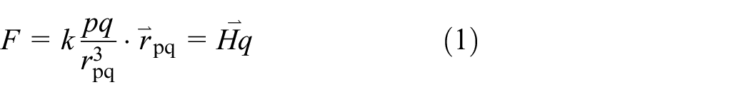
F = k \frac{pq}{r_{pq}^{3}} \cdot {\overset{⇀}{r}}_{pq} = \overset{⇀}{Hq}

(1)

where, k is the proportionality constant; r_pq is the distance between the magnetic-charge-points p and q; ${\overset{⇀}{r}}_{pq}$ is the vector between the magnetic-charge-points p and q; $\overset{⇀}{H}$ is the magnetic field strength of the magnetic field; p is the magnetic charge amount of the magnetic-charge-point p; q is the magnetic charge amount of the magnetic-charge-point q.

If the coordinate of the magnetic-charge-point p is (x_p,y_p,z_p), and the coordinate of the magnetic-charge-point q is (x_q,y_q,z_q), then $\overset{⇀}{r}$ of the magnetic-charge-points p and q can be expressed as:

\begin{matrix} {\overset{⇀}{r}}_{pq} = k_{1} \overset{⇀}{i} + k_{2} \overset{⇀}{j} + k_{3} \overset{⇀}{k} \\ k_{1} = (x_{p} - x_{q}) \\ k_{2} = (y_{p} - y_{q}) \\ k_{3} = (z_{p} - z_{q}) \end{matrix}

(2)

where, $\overset{⇀}{i}$ is the unit vector in the X-axis direction; $\overset{⇀}{j}$ is the unit vector in the Y-axis direction; $\overset{⇀}{k}$ is the unit vector in the Z-axis direction.

The proportionality constant k is expressed as:

k = \frac{1}{4 π μ}

(3)

where, μ is the magnetic permeability in the medium.

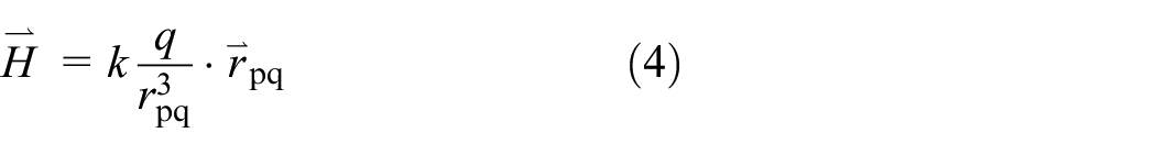
The magnetic field strength $\overset{⇀}{H}$ of the magnetic field is expressed as:

\overset{⇀}{H} = k \frac{q}{r_{pq}^{3}} \cdot {\overset{⇀}{r}}_{pq}

(4)

Analogous to the electric field, the smallest unit of the magnetic medium is regarded as a magnetic dipole. The orientation of the unmagnetized magnetic dipoles is chaotic. The magnetized magnetic dipoles are arranged in an orderly manner, and the internal polarities (N poles S poles) cancel each other out. In addition, the magnetic medium has N pole and S pole after being magnetized, that is, it has two opposite magnetic charge surfaces. Therefore, only the magnetic force between each magnetic charge surface needs to be considered when calculating the magnetic force of the inner rotor on the outer slider.

Figure 4 shows equivalent schematic of permanent magnet (NdFeB35). The shapes of the permanent magnets are I-shaped (permanent magnets of the inner rotor) and Bar-shaped (permanent magnets of the outer slider). In addition, the surface of the permanent magnet is mainly composed of the magnetic charge surface perpendicular to the magnetization axis and the magnetic charge surface of the bevel face. However, the magnetic charge surface of the bevel face complicates the whole analytical process. In order to ensure the accuracy of the analytical results and simplify the analytical process, the magnetic charge surface of the bevel face is now equivalently converted into a magnetic charge surface perpendicular to the magnetization axis, as shown in Figure 4. In addition, in order to facilitate the analysis of the magnetic force of each magnetic charge surface, each magnetic charge surface is labeled. In order to facilitate the observation and analysis of the force between the magnetic charge surfaces, the established coordinate system and each diagonal coordinate are shown in Figure 5.

Figure 4.

Equivalent schematic of permanent magnet.

Figure 5.

Schematic diagram of the force between the magnetic charge surfaces.

According to the theory of magnetostatics, the magnetic-charge-microelements A and B on the magnetic charge surface in Figure 5 are:

{\begin{matrix} q_{A} = σ_{A} d_{sA} \\ q_{B} = σ_{B} d_{sB} \end{matrix}

(5)

where, q_A is the magnetic charge amount of magnetic charge microelement A; q_B is the magnetic charge amount of magnetic charge microelement B; σ_A is the magnetic charge density of magnetic charge microelement A; σ_B is the magnetic charge density of magnetic charge microelements B.

The magnetic charge densities σ_A and σ_B are expressed as:

{\begin{matrix} σ_{A} = μ_{0} \overset{⇀}{M} \cdot \overset{⇀}{n} = B_{r} \\ σ_{B} = μ_{0} \overset{⇀}{M} \cdot \overset{⇀}{n} = B_{r} \end{matrix}

(6)

where, $\overset{⇀}{M}$ is the magnetization intensity of the permanent magnet; B_r is the residual magnetic flux density of the permanent magnet; $\overset{⇀}{n}$ is the unit vector in the normal direction; μ₀ is the air permeability.

The magnetic field strength of magnetic charge A at point B is expressed as:

{\overset{⇀}{H}}_{Q} = k \frac{q_{A}}{r_{AB}^{3}} \cdot {\overset{⇀}{r}}_{AB}

(7)

where, ${\vec{H}}_{Q}$ is the magnetic field strength of magnetic charge A at point B; r_AB is the distance between the magnetic-charge-microelements A and B; ${\overset{⇀}{r}}_{AB}$ is the vector between the magnetic-charge-microelements A and B; q_A is the magnetic charge amount of the magnetic-charge-microelement A.

According to equation (1), the magnetic force of magnetic-charge-microelement B received by magnetic-charge-microelement A can be expressed as:

d \overset{⇀}{F} = {\overset{⇀}{H}}_{Q} q_{B} = k \frac{B_{r}^{2} d_{sA} d_{sB}}{r_{AB}^{3}} \cdot {\overset{⇀}{r}}_{AB}

(8)

where, q_B is the magnetic charge amount of the magnetic-charge-microelement B.

Since the component forces projected by $d \overset{⇀}{F}$ on the X and Z axes can generate torque, only the component forces on the X and Z axes need to be considered in the calculation of the component forces. According to Figure 5, the magnetic force in the Z-axis direction can be obtained by integrating equation (8):

\begin{matrix} F Z_{nm} = \int_{x_{n}}^{x_{n}^{'}} \int_{y_{n}}^{y_{n}^{'}} \int_{x_{m}}^{x_{m}^{'}} \int_{y_{m}}^{y_{m}^{'}} k \frac{B_{r}^{2}}{r_{pq}^{3}} \overset{⇀}{k} \cdot {\overset{⇀}{r}}_{pq} d x_{p} d y_{p} d x_{q} d y_{q} \\ = \int_{x_{n}}^{x_{n}^{'}} \int_{y_{n}}^{y_{n}^{'}} \int_{x_{m}}^{x_{m}^{'}} \int_{y_{m}}^{y_{m}^{'}} g (x_{p}, y_{p}, x_{q}, y_{q}) d x_{p} d y_{p} d x_{q} d y_{q} \end{matrix}

(9)

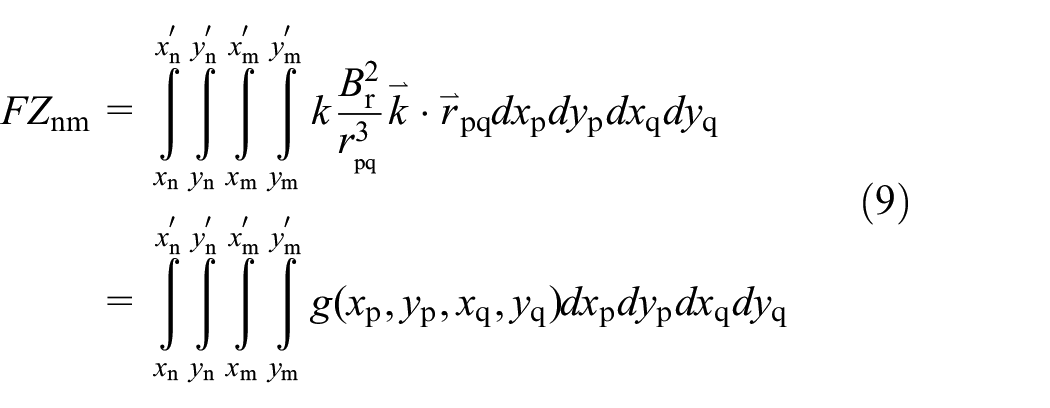
where, n is the label of each surface in Figure 4; m is the label of each surface in Figure 4; FZ_nm is the magnetic component force generated along the Z-axis direction between the labeled n surface and the labeled m surface (when the polarity of the two face surfaces is the same, the direction of the magnetic force is negative).

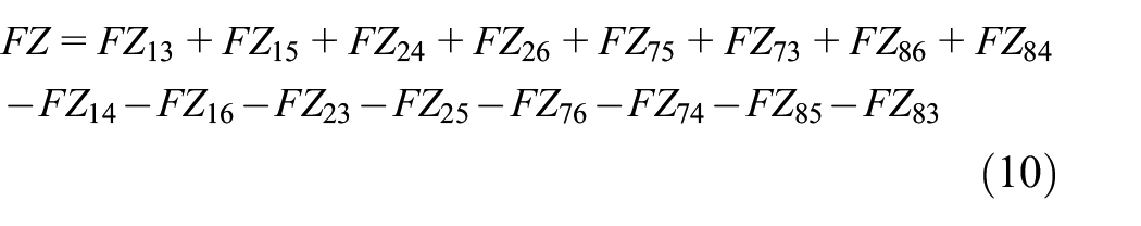
According to equation (9), the resultant force of the inner rotor in the Z-axis direction can be expressed as:

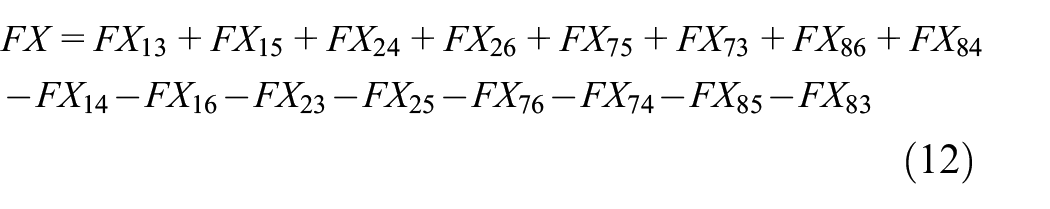
\begin{matrix} FZ = F Z_{13} + F Z_{15} + F Z_{24} + F Z_{26} + F Z_{75} + F Z_{73} + F Z_{86} + F Z_{84} \\ - F Z_{14} - F Z_{16} - F Z_{23} - F Z_{25} - F Z_{76} - F Z_{74} - F Z_{85} - F Z_{83} \end{matrix}

(10)

According to Figure 5, the magnetic force in the X-axis direction can be obtained by integrating equation (8):

\begin{matrix} F X_{nm} = \int_{x_{n}}^{x_{n}'} \int_{y_{n}}^{y_{n}'} \int_{x_{m}}^{x_{m}'} \int_{y_{m}}^{y_{m}'} k \frac{B_{r}^{2}}{r_{pq}^{3}} \overset{⇀}{i} \cdot {\overset{⇀}{r}}_{pq} d x_{p} d y_{p} d x_{q} d y_{q} \\ = \int_{x_{n}}^{x_{n}'} \int_{y_{n}}^{y_{n}'} \int_{x_{m}}^{x_{m}'} \int_{y_{m}}^{y_{m}'} g (x_{p}, y_{p}, x_{q}, y_{q}) d x_{p} d y_{p} d x_{q} d y_{q} \end{matrix}

(11)

where, FX_nm is the magnetic component force generated along the X-axis direction between the labeled n surface and the labeled m surface.

According to equation (11), the resultant force of the inner rotor in the X-axis direction can be expressed as:

\begin{matrix} FX = F X_{13} + F X_{15} + F X_{24} + F X_{26} + F X_{75} + F X_{73} + F X_{86} + F X_{84} \\ - F X_{14} - F X_{16} - F X_{23} - F X_{25} - F X_{76} - F X_{74} - F X_{85} - F X_{83} \end{matrix}

(12)

Since there are quadruple integrals in equations (9) to (12), the calculation process is difficult. In order to simplify the calculation process, this paper uses the Monte Carlo method to carry out the numerical integral calculation, that is, the calculation process is transformed into the expected value of random sampling in the specified interval. For γ-fold integration, let Ds be a region of n-dimensional space, and the specific expression is written as:

I = \int \dots \int_{Ds} g (x_{1}, x_{2}, \dots x_{γ}) d x_{1} d x_{2}, \dots d x_{γ}

(13)

When using the Monte Carlo method for integral calculation, the first thing to do is to select an appropriate probability density function f(x). In this paper, the uniform distribution function is selected as the probability density function f(x). Therefore, a set of independent and identically distributed random variables {(x₁¹, x₂¹⋯x_γ¹), (x₁², x₂²⋯x_γ²), ⋯ (x₁^γ, x₂^γ⋯x_γ^γ)} are obtained. According to the law of large numbers, we can get:

\begin{matrix} I = \int \dots \int_{Ds} \frac{g (x_{1}, x_{2}, \dots x_{γ})}{f (x_{1}, x_{2}, \dots x_{γ})} f (x_{1}, x_{2}, \dots x_{γ}) d x_{1} d x_{2}, \dots d x_{γ} \\ = E [\frac{g (x_{1}, x_{2}, \dots x_{γ})}{f (x_{1}, x_{2}, \dots x_{γ})}] \approx \frac{| D |}{N} \sum_{i = 1}^{N} \frac{g ({x_{1}}^{i}, {x_{2}}^{i}, \dots {x_{γ}}^{i})}{f ({x_{1}}^{i}, {x_{2}}^{i}, \dots {x_{γ}}^{i})} \end{matrix}

(14)

where, D is the accumulation of the difference between the upper and lower limits of the integral variable; N is the sampling times.

Solving equations (9) to (12) according to equation (14), the torque of the inner rotor is obtained as:

M = (FX \cdot \cos α - FZ \cdot \sin α) R

(15)

where, α is the angle of MC (as shown in Figure 4); R is the average radius of the inner rotor.

Stability analysis of 2D-MC-PV

Working stability is the top priority to be considered when designing a control system. 2D-MC-PV can be regarded as a differential hydraulic cylinder controlled by a three-way flow rate valve, which is essentially a hydro-mechanical closed-loop servo control system, as shown in Figure 6. Generally, hydro-mechanical servo systems have less flexibility due to their strong dependence on certain structural parameters. It was thus important to establish stability criterion firstly and explore the influence that these structural parameters have on the working stability of 2D-MC-PV.

Figure 6.

Schematic diagram of hydro-mechanical closed-loop servo control system.

The linear displacement of L-EMC needs to be converted to rotation by MC. According to the geometric relationship between the outer slider and inner rotor, the relationship between the output angle β and input linear displacement x_i can be written as:

β = \arccos (\frac{x_{i} \tan α}{R})

(16)

where, x_i is the displacement of L-EMC.

When the spool rotates, the opening area of the orifices A and B will vary accordingly, and the variation scale can be denoted as Δh. Since the feedback mechanism of MC, Δh is related to both x_i and x_o, which can be expressed as:

Δ h = R_{s} \cos β = \frac{R_{s} (x_{i} - x_{o}) \tan α}{R}

(17)

where, R_s is the radius of the spool; x_o is the displacement of the spool.

Since the rotation angle of the spool is very small (0 < h < r), the opening area expressions of orifices A and B can be written as:

\begin{matrix} A_{A} (h) = - A_{B} (h) \\ = r^{2} \arccos (\frac{r - h}{r}) + W_{g} h - (r - h) \sqrt{r^{2} - {(r - h)}^{2}} \end{matrix}

(18)

where, h is the height that the spool rotates; r is the chamfering radius of the grooves A and B; W_g is the width of the grooves A and B.

To derive the transfer function of 2D-MC-PV, it is necessary to obtain the flow continuity equation of the pilot stage and the dynamic equation of the spool. The flow continuity equation can be expressed as:

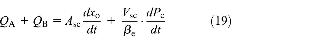
Q_{A} + Q_{B} = A_{sc} \frac{d x_{o}}{dt} + \frac{V_{sc}}{β_{e}} \cdot \frac{d P_{c}}{dt}

(19)

where, Q_A is the flow rate from the orifice A entering the chamber C; Q_B is the flow rate from the orifice B flowing out of the chamber C; A_sc is the force area of the chamber C; V_sc is the volume of the chamber C; β_e is the effective elastic bulk modulus.

The momentum balance equation of the spool can be expressed as:

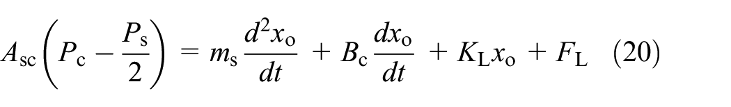
A_{sc} (P_{c} - \frac{P_{s}}{2}) = m_{s} \frac{d^{2} x_{o}}{dt} + B_{c} \frac{d x_{o}}{dt} + K_{L} x_{o} + F_{L}

(20)

where, m_s is the spool mass; B_c is the viscous damping coefficient of the load; K_L is the spring stiffness of the load; F_L is the external load force.

After Laplace transform, Equation (19) can be written as:

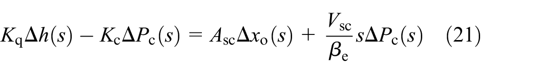
K_{q} Δ h (s) - K_{c} Δ P_{c} (s) = A_{sc} Δ x_{o} (s) + \frac{V_{sc}}{β_{e}} s Δ P_{c} (s)

(21)

where K_q is the flow coefficient; K_c is the flow-pressure coefficient.

Ignoring the influence of Coulomb friction force and flow force, the Laplace transformation of Equation (20) can be expressed as:

\begin{matrix} A_{sc} Δ P_{s} (s) = m_{s} s^{2} Δ x_{o} (s) + B_{c} s Δ x_{o} (s) \\ + K_{L} Δ x_{o} (s) + Δ F_{L} (s) \end{matrix}

(22)

Based on equations (21) and (22), the open-loop transfer function of 2D-MC-PV can be obtained as:

\begin{matrix} \frac{Δ x_{o} (s)}{Δ h (s)} = \\ \frac{A_{sc} K_{q}}{\frac{V_{sc}}{β_{e}} m_{s} s^{3} + (K_{c} m_{s} + \frac{V_{sc}}{β_{e}} B_{c}) s^{2} + (A_{sc}^{2} + B_{c} K_{c} + \frac{V_{sc}}{β_{e}} K_{L}) s + K_{L} K_{c}} \end{matrix}

(23)

Without considering the spring stiffness of the load, K_L = 0. Since B_cK_c≪A_sc², then the equation (23) can be simplified as:

\frac{Δ x_{o} (s)}{Δ h (s)} = \frac{1}{s} \cdot \frac{K_{q}}{A_{sc}} \cdot \frac{ω_{n}^{2}}{s^{2} + 2 ζ ω_{n} s + ω_{n}^{2}}

(24)

where, ζ is the damping ratio; ω_n is the natural frequency.

The Laplace transform of equation (17) can be obtained:

Δ h = \frac{R_{s} (Δ x_{i} (s) - Δ x_{o} (s)) \tan α}{R}

(25)

According to equations (24) and (25), the closed-loop transfer function of the 2D-MC-PV is obtained as:

\frac{Δ x_{o} (s)}{Δ x_{i} (s)} = \frac{R_{s} K_{q} \tan α}{R A_{sc}} \cdot \frac{ω_{n}^{2}}{s^{3} + 2 ζ ω_{n} s^{2} + ω_{n}^{2} s + \frac{R_{s} K_{q} \tan α}{R A_{sc}} ω_{n}^{2}}

(26)

According to equation (26), the characteristic equation of 2D-MC-PV can be expressed as:

\frac{1}{ω_{n}^{2}} s^{3} + \frac{2 ζ}{ω_{n}} s^{2} + s + K_{z} = 0

(27)

where, K_z is the proportional amplification factor.

K _z can be expressed as:

K_{z} = \frac{R_{s} A_{sc} K_{q} \tan α}{R}

(28)

According to equation (27), the following conditions must be met to stabilize the system:

2 ζ ω_{n} - K_{z} > 0

(29)

Finally, the stability criterion of 2D-MC-PV can be expressed as:

h_{0} > \frac{P_{s} L_{sc} R_{s} \tan α}{R β_{e}}

(30)

For the preliminary design of 2D-MC-PV the stability criterion showed in equation (30) must be given the priority since the structural parameters should meet equation (30) firstly in order to ensure valve working stability. Equation (30) also indicates the influence of crucial structural parameters on the working stability, which will be discussed in detail together with multi-objective optimization design in the next section.

Multi-objective optimization

Optimization design variables

During the optimization process, the parameters L_sc, α, W_g, and h₀ are selected as design variables. The reasons for choosing these four parameters are listed as follows:

From equation (30), the initial height of the overlapping area h₀ was found to be crucial to the characteristics of the valve. h₀ is not only related to multiple performance indexes including stability, valve dynamics, and pilot stage leakage, but also convenient from the point view of manufacturing in case that it needs to be adjusted for the purpose of optimization. Increasing h₀ increase both stability and dynamic response, however it also increases leakage of pilot stage.

The key parameter to improve valve dynamic characteristics is the width of the high- and low-pressure grooves W_g. An increase in W_g increases the flow rate of orifice A and orifice B of pilot stage, which accelerates the oil filling speed of the sensitive chamber, and thus improves the whole dynamic response. However, it also increases the pilot stage leakage.

Pitch angle α indicates the scale between the rotation of output armature and the linear displacement of input armature. Small scale benefits the control precision but reduces the dynamic response of output armature. In contrary, large scale improves the dynamic performance but demands high-accuracy control of proportional solenoid. Besides, according to equation (30), an increase in α deteriorates the valve stability.

Depth of sensing chamber L_sc had a significant influence on the stability of the spool. An increase in L_sc decrease the hydraulic natural frequency ω_n, decreasing the stability of the valve.

According to the 2D-MC-PV operating conditions, the ranges of selected parameters are shown in Table 1.

Table 1.

Ranges of selected parameters.

Parameters	h ₀(mm)	W _g (mm)	L _sc (mm)	α (rad)
Range	[0.1, 0.6]	[2, 8]	[2.5, 5]	[0.262, 0.785]

Optimization objective functions

The optimization objectives should be able to accurately represent the static/dynamic characteristics of 2D-MC-PV. In this study, the step response and the pilot stage leakage flow are combined used to reflect the optimization objectives, as shown in Figure 7. Here, t₀ is the excitation point of step response; t₁ is the rise time of the step response; t₂ is the settling time of the step response; t₃ is the cut off time for the step response; x_∞ is the stable value of the step response; Q_pilot is the pilot stage leakage flow rate. The step response speed of 2D-MC-PV is reflected by the rise time T_r since smaller T_r represents a faster dynamic response; the stability of 2D-MC-PV is reflected by the settling time T_s as smaller T_s means the response curve converges to the stable value x_∞ more rapidly; the static position accuracy of 2D-MC-PV is reflected by the stable value x_∞ because the closer x_∞ to 1 represents the higher position accuracy of 2D-MC-PV; the energy consumption of 2D-MC-PV is reflected by the pilot stage leakage flow Q_pilot since smaller Q_pilot represents the lower energy consumption of 2D-MC-PV.

Figure 7.

Schematic diagram of optimization objectives: (a) step response curve and (b) pilot stage leakage flow rate curve.

The relationship between the performance of 2D-MC-PV and the parameters L_sc, α, W_g, and h₀ is complex and contradictory. Therefore, it is difficult to choose a suitable set of values. To obtain optimization results with appropriate emphasis on performance, the response speed, stability, accuracy, and energy consumption are evaluated with different weight coefficients through J₁, J₂, J₃, and J₄ respectively. Therefore, the optimization objective function is defined as:

{\begin{matrix} J_{1} = 5 C_{1} T_{r} \\ J_{2} = 5 C_{2} T_{s} \\ J_{3} = C_{3} \frac{1}{x_{\infty}} \\ J_{4} = C_{4} Q_{pilo} \\ C_{1} + C_{2} + C_{3} + C_{4} = 1 \\ J = J_{1} + J_{2} + J_{3} + J_{4} \end{matrix}

(31)

In equation (31), J₁ is used to evaluate the response speed, where the smaller J₁ represents the faster step response of 2D-MC-PV; J₂ is used to evaluate the stability, where the smaller J₂ represents the more stable step response of 2D-MC-PV; J₃ is used to evaluate the steady-state value, where the smaller J₃ represents the smaller step response error of 2D-MC-PV; J₄ is used to evaluate the pilot stage leakage, where the smaller J₄ represents the smaller pilot stage leakage flow of 2D-MC-PV. If the sum of the coefficients of C₁, C₂, and C₃ is greater than 0.5, the combination of parameters aims at improving the dynamic performance of 2D-MC-PV; if the coefficient of C₄ is greater than 0.5, these parameters aim at reducing the energy consumption of 2D-MC-PV (low pilot stage leakage flow). Furthermore, if the proportion of C₁ is the largest among C₁, C₂, and C₃, it is intended to optimize the speed of the step response; if the proportion of C₂ is the largest among C₁, C₂, and C₃, it is intended to optimize the stability of the step response; if the proportion of C₃ is the largest among C₁, C₂, and C₃, it is intended to optimize static accuracy of the step response. Finally, J represents the comprehensive index, where the smaller J means that the optimization result is closer to the expectation.

Optimization method

The parameter optimization of 2D-MC-PV is a typical multi-objective optimization problem. In this section, a particle swarm optimization (PSO) algorithm is employed to solve this problem since it has excellent global convergence speed and simplicity.^33–35 Figure 8 shows the AMESim/Simulink co-simulation model of 2D-MC-PV.

Figure 8.

AMESim/Simulink co-simulation model of 2D-MC-PV.

The main parameters of PSO are as follows: the number of particles is 25, and the maximum number of optimizations is set to 50. Figure 9 shows the block diagram of the whole optimization process. After initializing the particle swarm, the Matlab scripts inputs the particle swarm into the co-simulation model to calculate the fitness value. If the fitness value satisfies the Hurwitz stability criterion (equation (30)), it will be returned to the Matlab main program for update of optimal value, particle position, and particle velocity. If the number of iterations is less than the maximum number of optimizations, the Matlab scripts continues to input the new particle swarm into the co-simulation model to calculate the fitness value, which will not stop until the maximum number of optimizations is reached. Then the optimal solution will be output.

Figure 9.

Block diagram of the optimization.

Table 2 gives other design parameters of 2D-MC-PV except for the above mentioned L_sc, α, W_g, and h₀. According to different optimization requirements, several combinations of the weight coefficients are considered and listed in Table 3. Since Case 1 and Case 2 focus on the optimization of dynamic characteristics, the sum of the coefficients C₁, C₂, and C₃ is 0.6, and C₄ is 0.4. Among them, Case1 needs to consider the high response speed, thus C₁ is 0.3, C₂ is 0.2, and C₃ is 0.1; Case 2 needs to consider both response speed and stability, thus C₁ is 0.2, C₂ is 0.3, and C₃ is 0.1. Since Case 3 focuses on the optimization of static characteristics, the sum of the coefficients C₁, C₂, and C₃ is 0.4, and C₄ is 0.6. In addition, to ensure the response speed and stability of the step response of Case3, C₁ is 0.15, C₂ is 0.15, and C₃ is 0.1.

Table 2.

Other design parameters of 2D-MC-PV.

Parameters	R	R _s	m _s	r
Value	25 mm	9 mm	0.3 kg	0.5 mm

Table 3.

Combinations of weighting coefficient.

Coefficients	C ₁	C ₂	C ₃	C ₄
Case 1	0.3	0.2	0.1	0.4
Case 2	0.2	0.3	0.1	0.4
Case 3	0.15	0.15	0.1	0.6

Results discussion

The final optimization results of the four optimization parameters L_sc, α, W_g, and h₀ are shown in Figure 10. The proposed optimization scheme can quickly find a set of optimal fitness values that meet the optimization expectations. With these optimized parameters the step response curve and pilot stage flow curve are simulated again by co-simulation model, as shown in Figure 11. Here the optimization result of Case 1 satisfies the index of high response speed; the result of Case 2 satisfies the index of high response speed and fast stability; the result of Case 3 satisfies the index of low energy consumption. The detailed optimization results are summarized in Table 4. Generally, larger h₀, W_g, and α are beneficial to improve the step response, but the increase of h₀ and W_g will increase the pilot stage leakage; the increase of L_sc is detrimental to the valve stability. Since Case 1 mainly focuses on the dynamic response at cost of the pilot stage leakage, the rise time T_r of Case 1 is significantly faster than that of Case 2 and Case 3, and Case 1 has obvious overshoot, which makes the setting time T_s too large. In addition, Case 3 mainly focuses on reducing the pilot stage leakage Q_pilot, therefore, the values of h₀ and W_g are too conservative. Thus, the rise time T_r and settling time T_s of Case 3 are much larger than that of Case 1 and Case 2. Since the C₃ of Case 1, Case 2, and Case 3 are all 0.1, the final stable value x_∞ is relatively close. Compared with Case 1 and Case 3, Case 2 can have a smaller pilot stage leakage while still ensuring good dynamic characteristics. Thus, Case 2 is finally selected as the design parameters reference of 2D-MC-PV prototype.

Figure 10.

Optimization process of parameters: L_sc, α, W_g, and h₀: (a) h₀, (b) W_g, (c) α, and (d) L_sc.

Figure 11.

Final optimization results: (a) step response curve and (b) pilot stage flow curve.

Table 4.

Summary of optimization results.

Parameters	h ₀ (mm)	W _g (mm)	α (rad)	L _sc (mm)	T _r (ms)	T _s (ms)	x _∞ (mm)	Q _pilot (L/min)
Case 1	0.29	4.71	0.78	3.85	27.6	68.3	0.995	0.38
Case 2	0.20	3.70	0.63	3.55	36.8	41.3	0.980	0.22
Case 3	0.14	4.25	0.61	3.2	79.2	127.3	0.966	0.18

Resistance torque calculation

In order to design a MC that can drive the spool to rotate, the resistance torque of the spool is calculated based on Fluent software. The resistance torque is mainly generated by the pilot stage of 2D-MC-PV. The resistance generated by the pilot stage has axial, radial, and circumferential components relative to the axial direction of the spool. Among them, the circumferential component force is the main factor hindering the rotation of the spool. In this paper, Fluent software is used to calculate the resistance torque of the spool. According to the dimensional parameters in Tables 2 and 4, SolidWorks software was used to build a 3D fluid model of the pilot stage. The dimensional parameters settings are shown in Table 5. Since the oil supply channel, the groove A, the groove B, and the flow-channel are all regular geometries, the hexahedral element with a grid of 0.4 mm is used to mesh the 3D fluid model of the pilot stage using Fluent software, as shown in Figure 12. And, the number of cells in the grid is 410129, the number of nodes is 83532, and the average grid quality is 0.826, which meets the CFD solution accuracy requirements. In the Fluent software, set the fluid medium as ISO VG 32 hydraulic oil (density of 873 kg/m³, viscosity of 0.0279 kg/m/s), and set up transient model and k-ε model. In addition, define the oil supply channel as the entrance, define the groove B as the export, and the other surfaces are wall surfaces, as shown in Figure 12.

Table 5.

Dimensional parameters.

Parameters	W _s (mm)	r (mm)	W _g (mm)	h ₀ (mm)
Value	4	0.5	4.25	0.14

Figure 12.

3D model of pilot stage of 2D-MC-PV.

Figure 13 shows the curve of the resistance torque changing with the opening of the pilot stage when the supply pressure is 10, 15, and 20 MPa respectively. The statistics of the maximum resistance torque obtained by Fluent software are shown in Table 6. In the pilot stage of 2D-MC-PV, the circumferential component force generated by the groove A and B forms a resistance torque (the direction of the resistance moment at the groove A is opposite to that at the groove B), which prevents the pilot stage from opening. When the opening of the pilot stage changes to 0 (the opening of the orifice A is equal to the orifice B), the pressure difference between the groove A and the flow-channel is P_s/2, and the pressure difference between the groove B and the flow-channel is P_s/2. At this time, the resistance torque at the groove A is basically the same as that at the groove B (the resistance torque M_r is the smallest). As the opening of the pilot stage increases (the orifice A becomes larger and the orifice B decreases), the pressure of the chamber C, and the resistance torque gradually increases to the maximum. When the resistance torque reaches the maximum (the orifice B is close to closing), the flow from the groove A into the chamber C decreases, the flow from the chamber C out of the groove B decreases, and the pressure of the chamber C approaches P_s.

Figure 13.

Resistance torque changing curve.

Table 6.

Maximum resistance torque.

Supply pressure (MPa)	10	15	20
Maximum resistance torque (Nm)	0.045	0.092	0.138

In this paper, the maximum resistance torque (M_r = 0.138 N/m) under 20 MPa is used as the design reference for MC. Since certain errors in the actual processing and assembly process, MC is designed according to 150% of the minimum output torque. According to equation (15) and the minimum output torque M_r calculated by Fluent software, the main parameters of the designed MC are shown in Table 7. In addition, MC is simulated and analyzed by MAXWELL software, and the comparison between the simulation results (SIM) and the analytical results (ANA) is shown in Figure 14. It can be seen that the simulation results are in good agreement with the analytical results, indicating that the equation (15) can provide effective theoretical guidance for the design of MC.

Table 7.

Main parameters of the designed MC.

3D model	Parameters	Value
	h ₁ (mm)	4
	L ₁ (mm)	25
	W ₁ (mm)	20
	R (mm)	28
	δ (mm)	1
	h ₂ (mm)	2.5
	h ₃ (mm)	3
	L ₂ (mm)	25
	W ₂ (mm)	18

Figure 14.

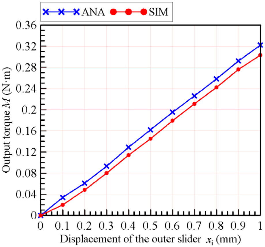
Displacement-torque curve of MC.

Experimental Study

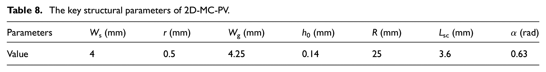
According to Hurwitz stability criterion, multi-objective optimization results and Fluent finite element simulation results, a 2D-MC-PV prototype is designed and processed, as shown in Figure 15. In addition, the key structural parameters of the prototype are shown in Table 8. Anyang’s proportional solenoid (GP45A4-AIW9) is selected for L-EMC. The main characteristics of proportional electromagnet are shown in Table 9. In order to test the static and dynamic characteristics of the 2D-MC-PV prototype, a special experimental platform was built. The hydraulic circuit of the experimental platform is shown in Figure 16. Figure 17 illustrates the experimental platform for 2D-MC-PV, which mainly includes 2D-MC-PV prototype, flow meter, pressure gauge, proportional amplifier, oscilloscope, signal generator, and displacement sensor.

Table 8.

The key structural parameters of 2D-MC-PV.

Parameters	W _s (mm)	r (mm)	W _g (mm)	h ₀ (mm)	R (mm)	L _sc (mm)	α (rad)
Value	4	0.5	4.25	0.14	25	3.6	0.63

Figure 15.

Prototype of 2D-MC-PV.

Table 9.

Main characteristics of GP45A4-AIW9 .³⁸

Performance	Force (N)	Current (A)	Resistance (Ω)	Stroke (mm)	Hysteresis (%)	Linearity (%)
Value	80	0.8	19.5	±3	≤3%	≤1%

Figure 16.

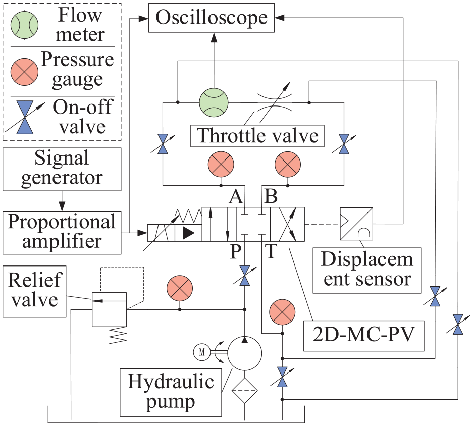
Hydraulic circuit of the experimental platform.

Figure 17.

Experimental platform for 2D-MC-PV.

Static characteristics

Table 10 summarizes the experimental and simulation results of the static characteristics at supply pressures of 10, 15, and 20 MPa (the simulations are based on the AMESim model in Figure 8), including the maximum no-load flow, maximum leakage flow and hysteresis. Figure 18 shows the experimental (EXP) and simulated (SIM) no-load flow characteristic curves. When the oil supply pressure is 10, 15, and 20 MPa, the maximum no-load flow measured by experiment are 62.5, 78.9, and 108.8 L/min, respectively; the maximum no-load flow obtained by simulation are 66.8, 84.5, and 117.5 L/min, respectively; the hysteresis measured by experiment are 5.20%, 4.18%, and 3.36%, respectively; the hysteresis obtained by simulation are 1.02%, 0.88%, and 0.75%, respectively. It can be seen that the maximum flow rate increases with the increase of oil supply pressure. In addition, 2D-MC-PV prototype still has good static characteristics without any chatter compensation and other closed-loop feedback controls. Since the AMESim model does not consider the errors of processing and assembly and the pressure loss of the flow path, the flow rate obtained by simulation is larger than that measured by experiment, and the hysteresis obtained by simulation is much smaller than that measured by experiment. In addition, with the increase of supply pressure, the hysteresis of 2D-MC-PV becomes slightly smaller, and it is basically controlled below 2%, which meets the requirements of proportional control. Figure 19 shows the leakage flow curves, the peak of the pulse waveform represents the leakage flow, which includes the leakage flow from the power stage and the pilot stage. When the oil supply pressure is 10, 15, and 20 MPa, the leakage flow measured by experiment are 3.46, 4.58, and 7.12 L/min, respectively; the leakage flow obtained by simulation are 1.02, 2.85, and 5.08 L/min, respectively. Since the small opening between the groove A, the groove B, and the flow-channel, the leakage flow of the pilot stage is almost zero. This shows that the 2D-MC-PV has less zero-position power loss (reduced useless energy consumption). Since the AMEsim model does not consider the errors of processing and assembly, the simulation results are smaller than the experimental results. The above results fully verify that 2D-MC-PV has good static characteristics and can realize proportional control of high pressure and large flow.

Table 10.

Experimental results of static properties.

Supply pressure (MPa)		10	15	20
Maximum no-load flow (L/min)	EXP	62.5	78.9	108.8
Maximum no-load flow (L/min)	SIM	66.8	84.5	117.5
Leakage flow (L/min)	EXP	3.46	4.58	7.12
Leakage flow (L/min)	SIM	1.42	2.85	5.08
Hysteresis (%)	EXP	5.20	4.18	3.36
Hysteresis (%)	SIM	1.02	0.88	0.75

Figure 18.

No-load flow characteristic curves.

Figure 19.

Leakage flow curves.

Dynamic characteristics

Table 11 summarizes the experimental and simulation results of the dynamic characteristics under the oil supply pressure of 10, 15, and 20 MPa, including the amplitude-frequency width, phase-frequency width, and step response rise time. Figure 20 shows the experimental and simulated step response curves. When the oil supply pressure is 10, 15, and 20 MPa, the rise times measured by experiment are 132.1, 82.6, and 52.8 ms, respectively; the rise times obtained by simulation are 128.2, 75.8, and 41.3 ms, respectively. While for 20 MPa, the step response curve shows obvious overshoot, which is in good agreement with the simulation results. An increase in supply pressure leads to 2D-MC-PV instability, which verifies the correctness of the stability criterion. In addition, the dynamic performance of 2D-MC-PV can be further improved if a higher-frequency electromechanical converter is used as the actuator. Figure 21 shows the experimental and simulated amplitude-frequency characteristic curves and phase-frequency characteristic curves. When the oil supply pressure is 10, 15, and 20 MPa, the amplitude-frequency widths (up to −3 dB) measured by experiment are 17.5, 24.6, and 27.8 Hz, respectively; the amplitude-frequency widths obtained by simulation are 19.6, 25.2, and 32.5 Hz, respectively; the phase-frequency widths (up to −90°) measured by experiment are 21.8, 29.8, and 36.6 Hz, respectively; the phase-frequency widths obtained by simulation are 24.2, 32.6, and 42.3 Hz, respectively. It can be seen that the amplitude-frequency width and the phase-frequency width increase with the increase of the oil supply pressure. In addition, 2D-MC-PV has good tracking characteristics at low frequency. The simulation results of frequency characteristics and step response characteristics are in good agreement with the experimental results, indicating that AMESim model can provide effective theoretical guidance for 2D-MC-PV design.

Table 11.

Experimental results of dynamic properties.

Supply pressure (MPa)		10	15	20
Step response rise time (ms)	EXP	132.1	82.6	52.8
Step response rise time (ms)	SIM	128.2	75.8	41.3
Amplitude-frequency width (Hz)	EXP	17.5	24.6	27.8
Amplitude-frequency width (Hz)	SIM	19.6	25.2	32.5
Phase-frequency width (Hz)	EXP	21.8	29.8	36.6
Phase-frequency width (Hz)	SIM	24.2	32.6	42.3

Figure 20.

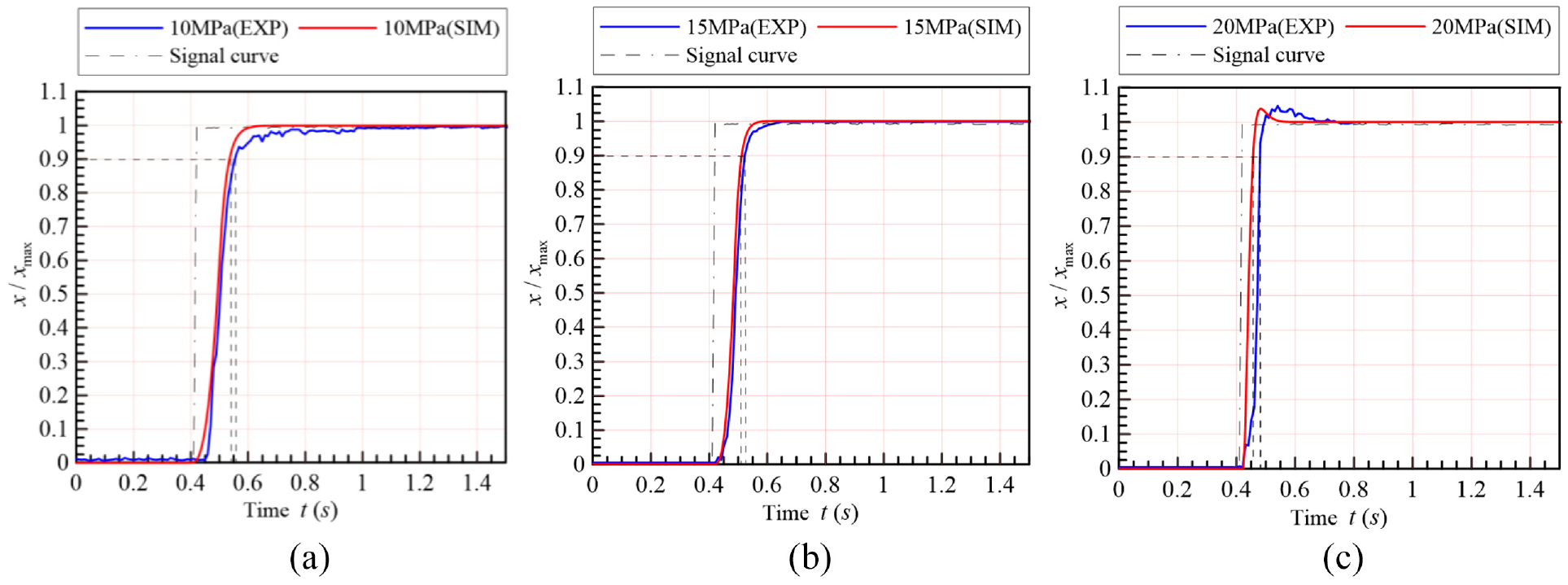
Step response curves: (a) 10 MPa, (b) 15 MPa, and (c) 20 MPa.

Figure 21.

Frequency response characteristic curves: (a) amplitude-frequency characteristic and (b) phase-frequency characteristic.

Conclusions

As a hydro-mechanical servo system, the whole performance of the 2D-MC-PV highly depend on certain structural parameters. To tradeoff good static/dynamic characteristics, good working stability and low leakage pilot stage, a multi-objective optimization is inevitable for preliminary design stage. Therefore, this paper proposes a multi-objective optimization method based on AMESim and Matlab/Simulink co-simulation model, which optimizes key structural parameters by adjusting weight coefficients (balancing static, dynamic, and pilot leakage performance). The multi-objective optimization method proposed in this paper successfully combines the advantages of AMESim and Matlab/Simulink, making up for the shortcomings. Finally, the optimized parameters are used for the design and manufacture of the 2D-MC-PV hydraulic part.

In order to design a MC that can drive the spool to rotate, the analytical equation of MC is derived based on the Coulomb’s law and the law of equivalent magnetic charge, and the Monte Carlo method is used to calculate. According to the resistance torque of the spool calculated by the Fluent software and the angle α of MC obtained by multi-objective optimization, a magnetic repulsion coupling is designed.

The 2D-MC-PV prototype was obtained by assembling the machined MC with the machined 2D-MC-PV hydraulic part. A special experimental platform was built to test the 2D-MC-PV prototype. During the experiment, MC can quickly drive the spool to rotate. The experimental results show that under the oil supply pressure of 20 MPa, the maximum flow rate can reach 108.8 L/min, the hysteresis is 3.36%, the amplitude-frequency width is 27.8 Hz, and the phase-frequency width is 36.6 Hz. It can be seen that the static and dynamic performance of the 2D-MC-PV prototype meets the requirements of the civil electro-hydraulic system. On the one hand, it is shown that the analytical equation of MC proposed in this paper can be used as an effective theoretical guide for the design of the MC. On the other hand, it shows that the multi-objective optimization method proposed in this paper can be used as an optimization method for 2D-MC-PV.

Footnotes

Appendix

Handling Editor: Chenhui Liang

Declaration of conflicting interests

The author(s) declared no potential conflicts of interest with respect to the research, authorship, and/or publication of this article.

Funding

The author(s) disclosed receipt of the following financial support for the research, authorship, and/or publication of this article: The research work is supported by the National Natural Science Foundation of China (Grant Nos. 51975524, 51405443) and National Key Research and Development Program (Grant No. 2019YFB2005201).

ORCID iDs

Hao Xu

Bin Meng

References

Tamburrano

Plummer

Distaso

, et al. A review of electro-hydraulic servovalve research and development. Int J Fluid Power 2019; 20: 53–98.

Montgomery

Smith

MB.

Hydraulic fracturing: History of an enduring technology. J Pet Technol 2010; 62: 26–40.

Shen

Liu

, et al. Research and development of electro-hydraulic control valves oriented to industry 4.0: a review. Chin J Mech Eng 2020; 33: 29.

Zhang

Qian

, et al. Influence of pre-stage cavitation on performance of double-nozzle flapper pressure servo valves. Proc IMechE, Part C: J Mechanical Engineering Science 2021; 235: 6822–6832.

Zhang

Huang

, et al. Design and verification of two-stage brake pressure servo valve for aircraft brake system. Processes 2021; 9: 979.

Yang

Review of Intelligent manufacturing and intelligent hydraulic components. Chin Hydraul Pneum 2020; 1: 1–9.

Tamburrano

Plummer

Distaso

, et al. A review of direct drive proportional electrohydraulic spool valves: industrial state-of-the-art and research advancements. J Dyn Syst Meas Control 2019; 141: 020801.

Cristofori

Vacca

The modeling of electrohydraulic proportional valves. J Dyn Syst Meas Control 2012; 134: 021008.

Amirante

Moscatelli

Catalano

LA.

Evaluation of the flow forces on a direct (single stage) proportional valve by means of a computational fluid dynamic analysis. Energy Convers Manag 2007; 48: 942–953.

10.

Amirante

Catalano

Poloni

, et al. Fluid-dynamic design optimization of hydraulic proportional directional valves. Eng Optim 2014; 46: 1295–1314.

11.

Zhao

Liao

Lian

, et al. Research on the performance of a novel electro-hydraulic proportional directional valve with position-feedback groove. Proc IMechE, Part E: J Process Mechanical Engineering 2021; 235: 1930–1944.

12.

Eryilmaz

Wilson

BH.

Unified modeling and analysis of a proportional valve. J Franklin Inst 2006; 343: 48–68.

13.

Meng

Heng

Novel modulation approach of flat force–displacement characteristic of linear electro-mechanical converter for electro-hydraulic servo-proportional valve. Proc IMechE, Part I: J Systems and Control Engineering 2022; 236: 1922–1939.

14.

Deldar

Izadian

Vaezi

, et al. Modeling of a hydraulic wind power transfer utilizing a proportional valve. IEEE Trans Ind Appl 2015; 51: 1837–1844.

15.

Chen

Peng

Gao

, et al. Position control of direct-acting high-frequency proportional valve. Chinese Hydraulic & Pneumatics 2021; 2: 36.

16.

Wang

Huang

, et al. A novel control strategy for pilot controlled proportional flow valve with internal displacement-flow feedback. J Dyn Syst Meas Control 2018; 140: 111014.

17.

Gao

Zhu

, et al. Development of a novel two-stage proportional valve with a pilot digital flow distribution. Front Mech Eng 2021; 16: 420–434.

18.

Wang

Huang

, et al. Performance improvement of a two-Stage proportional valve with internal hydraulic position feedback. J Dyn Syst Meas Control 2021; 143: 071005.

19.

Wang

Huang

, et al. Flow control for a two-stage proportional valve with hydraulic position feedback. Chin J Mech Eng 2020; 33: 1–13.

20.

Ding

Zhang

, et al. Modeling and dynamic characteristics analysis on a three-stage fast-response and large-flow directional valve. Energy Convers Manag 2014; 79: 187–199.

21.

Zhang

, et al. Investigation on the dynamic characteristics and control accuracy of a novel proportional directional valve with independently controlled pilot stage. ISA Trans 2019; 93: 218–230.

22.

Ruan

Ukrainetz

Burton

Frequency domain modelling and identification of 2D digital servo valve. Int J Fluid Power 2000; 1: 49–59.

23.

Ruan

Burton

Ukrainetz

An investigation into the characteristics of a two dimensional “2D” flow control valve. J Dyn Syst Meas Control 2002; 124: 214–220.

24.

Zheng

Ding

, et al. Theoretical and experimental research on the cartridge two-dimensional (2D) electro-hydraulic servo valve. Adv Mech Eng 2021; 13: 1687814021996532.

25.

Design and study of large flow 2D eletro-hydraulic proportional directional valves. MSc Thesis, Zhejiang University of Technology, Hangzhou, 2013.

26.

Zuo

Sun

, et al. Experimental and numerical investigations of the ball-screw-type coupling in two-dimensional electro-hydraulic proportional directional valve. Adv Mech Eng 2018; 10: 1687814018802509.

27.

Liu

Research of key technologies of 2D electro-hydraulic proportional directional valve with displacement enlarging. PhD Thesis, Zhejiang University of Technology, Hangzhou, 2015.

28.

Bin

Hao

Jian

, et al. Theoretical and experimental investigation on novel 2D maglev servo proportional valve. Chin J Aeronaut 2021; 34: 416–431.

29.

Chen

Swarm intelligence in mechanical engineering. Adv Mech Eng 2016; 8: 1687814016683595.

30.

Brezočnik

Fister

Podgorelec

Swarm intelligence algorithms for feature selection: a review. Appl Sci 2018; 8: 1521.

31.

Slowik

Kwasnicka

Nature inspired methods and their industry applications—Swarm intelligence algorithms. IEEE Trans Ind Inform 2018; 14: 1004–1015.

32.

Parpinelli

Lopes

HS.

New inspirations in swarm intelligence: a survey. Int J Bioinspired Comput 2011; 3: 1–16.

33.

Banks

Vincent

Anyakoha

A review of particle swarm optimization. Part I: background and development. Nat Comput 2007; 6: 467–484.

34.

Wang

Tan

Liu

Particle swarm optimization algorithm: an overview. Soft Comput 2018; 22: 387–408.

35.

Seo

Heo

, et al. Multimodal function optimization based on particle swarm optimization. IEEE Trans Magn 2006; 42: 1095–1098.

36.

Giles

MB.

Multilevel monte carlo methods. Acta Numerica 2015; 24: 259–328.

37.

Kroese

Brereton

Taimre

, et al. Why the Monte Carlo method is so important today. WIREs Comput Stat 2014; 6: 386–392.

38.

Anyang Company. Screw proportional solenoid GP45-4-A, http://www.aykaidi.com/products/products344.html (2022, accessed 08 August 2022).

Multi-objective optimization design of two-dimensional proportional valve with magnetic coupling

Abstract

Keywords

Introduction

Configuration and working principle

Mathematical analytical model

Mathematical model of MC

Stability analysis of 2D-MC-PV

Multi-objective optimization

Optimization design variables

Optimization objective functions

Optimization method

Results discussion

Resistance torque calculation

Experimental Study

Static characteristics

Dynamic characteristics

Conclusions

Footnotes

Appendix

Declaration of conflicting interests

Funding

ORCID iDs

References