
Abstract
In this article, a network of central pattern generators is used for the motion planning of a hexapod robot. There are many parameters in the planning network, which determine the motion performance of the hexapod robot. On the other hand, the network is a highly nonlinear coupling network, which is difficult to obtain optimal parameters by an analytical method. Optimizing these parameters to make the robot walk well is a multi-objective optimization process. There is a certain mutual exclusion relationship among the targets. To find a well-performing network as soon as possible, a multi-objective genetic algorithm is used for the process of parameter tuning. The hexapod robot simulation model is performed in Webots, and the motion performance parameters of the robot are obtained through built-in sensors and are also considered as mean values of the optimization algorithm. The optimization algorithm is written and run with MATLAB. Finally, the optimization algorithm and simulation results are proven by an experiment.
Keywords
Introduction
The hexapod robot is one of the most important legged robots. Hexapod robots have better stability and flexibility compared with biped and quadruped robots. 1 –3 Even with a failed leg, the hexapod robot can go on walking. 4
The traditional hexapod robot motion law is determined through its kinematics and dynamics modeling. However, the implementation process is complicated and unstable. Compared with robots, animals in nature can achieve rhythmic, stable movements. Therefore, it is very beneficial to use a biological planning method for robot gait planning, which simulates the rhythmic movement of animals. Central pattern generators (CPGs) are primarily located in the relevant ganglia of the central nervous system of vertebrates or invertebrates. 5 In 1987, Matsuoka proposed the first practical CPG model. 6 It has been successfully applied to motion control, especially in the gait of different bionic robots, such as snake/fish robots, 7 humanoid robots, 8 and quadruped robots. 9 A challenge of investigating the CPG system is to design the nonlinear oscillator model together with the coupling terms so that the resulting outputs satisfy the requirements of gait generation. 10 Yu et al. 11 proposed a novel CPG-based control architecture for hexapod walking robot based on a modified Van der Pol oscillator. Zhong et al. 12 designed an adjustment function to modulate the phase signals generated by the CPG network based on Matsuoka’s neural oscillator.
Although the motion control with the CPG model has broad research prospects and value, it has some shortcomings. For example, it is difficult to find a suitable set of parameters in the vast parametric search space to generate the expected motion pattern. 13 In the construction of a CPG-based control network, it is necessary to adjust the model parameters of the CPG, such as frequency, amplitude, phase lag, and waveform. It is always a tedious task to optimize the parameters of a single CPG model and the coupling weights of the CPG network to achieve a good performance. Liu et al. 14 used a CPG composed of mutually coupled Hopf oscillators and realized the start and stop of movement by adjusting the parameters of the Hopf oscillator. Zhu et al. 15 proposed a novel σ-Hopf harmonic oscillator and a central pattern based on backward control, which the locomotion achieved in a fast, smooth, and stable way. It is difficult to obtain the analytical solution of the differential equation consist of a nonlinear Hopf oscillator. Therefore, it is an effective solution through professional computer software and simulation software. In this article, MATLAB is used to run the multi-objective genetic algorithm to optimize individual parameters. Webots (robot simulator) is used to achieve the motion performance parameters of the hexapod robot.
Currently, some studies optimized the CPG network model parameters of the robot based on evolutionary optimization algorithms. For biped robots, Wolff used evolutionary algorithms to optimize the parameters that need to be adjusted to achieve the desired robot velocity. 16 For quadruped robots, Oliveira et al. 17 considered four conflicting objectives, simultaneously: minimize the body vibration, maximize the velocity, the wide stability margin, and the behavioral diversity. Cristiano et al. 18 found out an optimal combination of internal parameters of the CPG given a desired walking speed in a straight line by a genetic algorithm. Robotic motion planning is a multi-target optimization problem with multiple conflicting goals that are needed to be considered simultaneously. Saputra uses the non-dominated sorting genetic algorithm II (NSGA-II) algorithm for biped robot motion planning, and its objective functions are energy consumption, stability, and velocity. 19 Oliveira et al. 20 use NSGA-II to optimize the synaptic weight of a quadruped robot (cat, dog), and its optimization target is the stability of the trunk, velocity, and movement direction. Zhang et al. 21 studied the optimal gait parameter combination of the three gaits of the eel robot based on the NSGA-II algorithm.
Our contribution to the locomotion of hexapod robots is that we implement the multi-objective evolutionary algorithm to optimize the best compromise between walking velocity and stability. The optimization of the robot’s target values (velocity, setback, bump) is achieved by optimizing the parameters of the CPG network oscillator.
This article is organized as follows. The second section discusses the framework of the CPG network. The third section gives the parameter optimization algorithm and simulation. The fourth section shows the experimental results. The fifth section gives the conclusion.
Framework of the CPG network
The traditional robot control law is obtained by building a kinematics and dynamics model which is difficult to implement and unstable. As a result, a control method for generating a rhythmic motion control signal from a neural network is proposed by Graham Brown, 22 Shik, which is named CPG, and it can generate rhythm signals in the absence of high-level commands and external feedback.
Mathematical model of a single CPG oscillator and analysis of parameters to be optimized
The Hopf oscillator model is a coupled oscillator model, and its model parameters have clear physical meanings and have the characteristics of fewer parameters and independent and adjustable oscillator amplitude and phase. We use the Hopf oscillator as a model for the gait generation of a hexapod robot. The mathematical model is shown as follows

where x and y are the two state variables of the Hopf oscillator, the amplitude of which is

Hopf oscillator output.
CPG network construction
The walking stability of the robot requires coordinated motion between the various limbs of the robot, which depends on the phase relationship between the oscillators that make up the CPG network. 6 In this article, six oscillators are used to construct a CPG symmetric network. As shown in Figure 2, each one of the six legs of the fully symmetric network is bidirectionally connected to the other five legs. Each oscillator corresponds to one leg, and the state values x, y of the oscillator output are mapped to the angle values of the knee joint, the hip joint, and the ankle joint through a mapping function.

Fully symmetric network and leg mapping.
The mathematical model of the coupling relationships of the fully symmetric network is constructed by the six Hopf oscillation, as shown in equation (2) 23
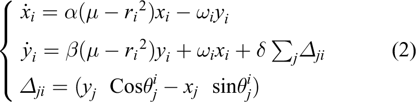
where
The state values x and y of the oscillator output need to be mapped to each joint angle in the joint space to make the robot walk normally. The angle values of the hip joint, the knee joint, and the ankle joint are represented by

where k is the proportionality factor and b is the biased value; k
0, k
1, k
2, b
0, b
1, and b
2 map x, y to the angle values of the hip joint and the knee joint; and k
3, k
4, b
3, b
4 map the knee joint angle value
Effect of parameters on CPG network output
The amplitude, frequency, and duty cycle of the two state variables x, y of the output can be changed by adjusting the Hopf oscillator parameters. The angles of the hip joint, knee joint, and ankle joint of the hexapod robot are mapped by the output states x, y through the linear converter. Therefore, we need to obtain a set of reasonable parameter ranges through analysis and avoid wasting time in the invalid search space when using the multi-objective genetic algorithm to optimize these parameters.
The α, β, μ, ω in the internal parameters of the Hopf oscillator are divided into three groups, and α = β is a group, and μ and ω are each a group. Keep μ = 1, ω = 1, t = 20, let α = β = 0.5, α = β = 10, respectively, and obtain two sets of output waveforms as shown in Figure 3.

The effect of different α and β values on the output waveform. (a)
It can be seen from Figure 3 that the output waveforms of the oscillator output state values x and y converge more when the values of α and β increase.
Suppose α = β = 1, ω = 1, and t = 20, respectively. Let μ = 1 and μ = 4, respectively, and obtain two sets of output waveforms as shown in Figure 4.

The effect of different μ on the output waveform. (a)
As seen from Figure 4, the amplitude of the oscillator output waveform is .
Keep α = β = 1, μ = 1, t = 20, and let ω = π, ω = 2π, respectively, and obtain two sets of output waveforms as shown in Figure 5.
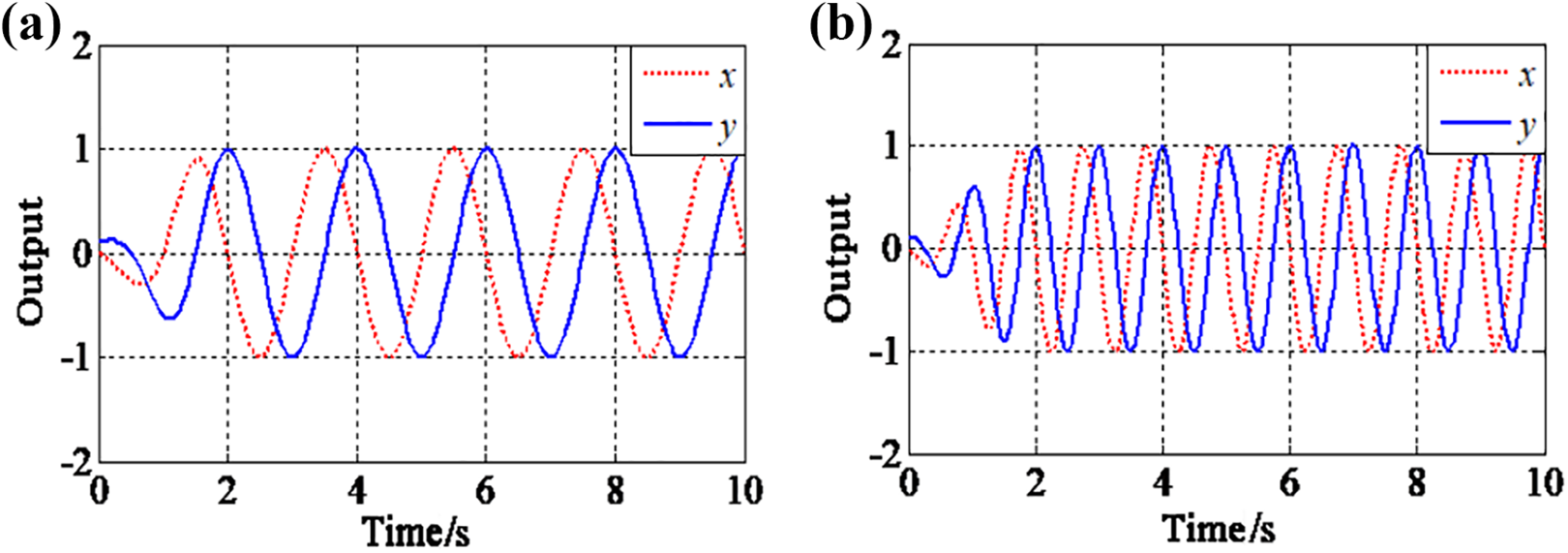
The effect of different ω on the output waveform. (a)
As can be seen from Figure 5, the frequency of the output waveform increases when ω increases.
Adjusting the parameters α, β, μ, ω, and δ in equation (2) and k 0, k 1, k 2, k 3, k 4 in equation (3) can change the moving performance of the hexapod robot. The hexapod robot gait is triple supporting, which needs to be optimized in this article.
Parameter optimization and simulation
The network of the CPG generates trajectories for the hexapod robot. Therefore, we must adjust the CPG parameters to change the three joint angles. We use an optimization algorithm framework based on multi-objective genetic to search for the optimal set of the CPG parameters.
Multi-objective genetic algorithm
Different from the single-objective genetic algorithm’s only certain solution, the multi-objective genetic algorithm often has multiple solutions.
In general, the multi-objective optimization problem with


where
In the decision space


Use
The objective function has the following characteristics. First, the unit of each objective function is different, so it can’t be compared simply. Second, each objective function will conflict with the other and cannot optimize at the same time, that is, improving the value of some objective function will damage the other objective function. Therefore, all objective functions cannot reach the optimal solutions at the same time. As a result, the Pareto optimal solution is introduced, which is defined according to the superior relation of the solution.
Without the loss of generality, for the minimization problem, the superiority relation is defined as follows. For
Range selection of parameters to be optimized
Proper parameter range selection can reduce searching time in unnecessary variable spaces. According to the case that has been successfully debugged, the range of the original CPG parameters is reduced or expanded by 10 times, and the search range of the optimization algorithm is formed, as shown in Table 1.
The range of optimized parameters.

Multi-objective optimization simulation and result analysis
As an evolutionary optimization algorithm, the multi-objective genetic algorithm does not search the global space. The solution obtained by this search method cannot be the global optimal solution. Therefore, the optimal solutions mentioned below are all local optimal solutions. The running process of the algorithm is random, and the optimal result of 10 runs is taken as the final result. The crossover probability was adjusted by stages, the mutation probability and elite retention probability are set to 0.1, and the population size and iteration times are set to 100.
The three target values needed to be optimized in the simulation are reciprocal velocity, the values of setback, and bump. And these three target values are related to the parameters of the CPG network in Table 1, so they are optimized by the CPG network parameters. To generalize the minimum optimization problem, the reciprocal of velocity is taken as the optimization objective. The formula is described as follows:

where
Taking into account the minimum and maximum values of the robot joint angles, inequality constraints are introduced to avoid invalid solutions. For the newly generated points in space S, the boundary constraints are as follows

where li , ui are the lower and upper limit of i component, respectively. The constraint handling method proposed by Deb 25 is used to handle inequality constraints. This method is based on a penalty function that does not require any penalty parameter. Careful comparisons among feasible and infeasible solutions are made so as to provide a search direction towards the feasible region.
The evolution curves of the three targets are shown in Figure 6. In Figure 6(a), the average and minimum values of the reciprocal velocity decrease uniformly from the beginning, and the convergence is completed after the 50th generation. Figure 6(b) shows that in the evolution curve of bump value, the distance between the minimum value and the average value is larger. In Figure 6(c), at first, the average value of bump value decreased, then rose to a top, and fell to a stable state finally. The minimum value of bump value first fluctuated, and finally the region was flat. Both reached a stable state after 50 generations. Figure 6(d) shows the relationship among the optimal individuals of the velocity inverse, setback, and bump in the three-dimensional space. The marks “*” represent the positions of the three optimal solutions in the initial population, and the marks “☆” represent the positions of the three optimal solutions of the last generation population. It can be seen from Figure 6 that the optimal solution of the last generation population is more dispersed than that of the initial population. To present the results more intuitively, the evolution curves of velocity reciprocal, setback value, and bump value are drawn in the three-dimensional diagram, as shown in Figure 7.
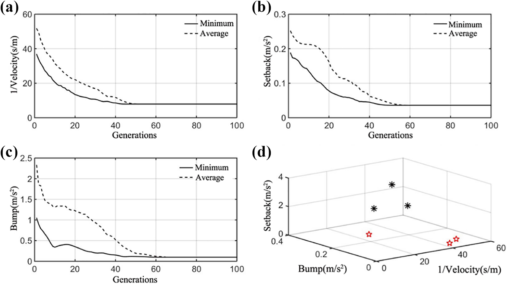
Effect of different values of the parameter ω on the setback and bump values. (a) Curve of velocity evolution; (b) curve of stepback evolution; (c) curve of bump evolution; and (d) nondominated solution of velocity, setback, and bump.
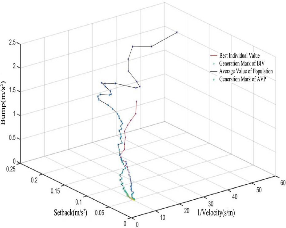
Three dimensional display of evolution of three objects.
The red line in Figure 7 represents the value evolution curve of an optimal individual in a single target, and “☆” represents the algebraic mark, and the color change indicates the algebraic change. The individuals with the color being close to blue mean the results that are closer to the first generation. On the contrary, the individuals with the color being close to yellow mean the results that are closer to the last generation.
In Figure 7, the black line represents the average evolution curve of a single target in the population, and “*” represents its algebraic mark. Its algebraic change is represented by the color change in the same way as that of the optimal individual. In the beginning, the distribution of the target value is relatively scattered. After a period of evolution, the optimal individual objective value and the population average value are all gathered toward the minimum direction.
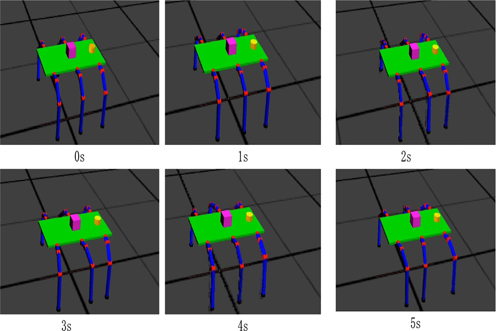
The motion process intercepted by the individual with the best running velocity in the simulation environment is shown in Figure 8.

Screenshot of the optimal individual simulation of velocity.
To obtain faster velocity, the hip joint of the robot needs to provide a larger rotation angle. It can be seen from Figure 8 that the swing amplitude of the hip joint and the locomotion distance of the robot are both large after each second. It also shows that the velocity of the robot in the simulation prototype depends on the rotation velocity of the hip joint and has nothing to do with the rotation of the knee and ankle joints.
The motion process intercepted by running the individual with the best setback value in the simulation environment is shown in Figure 9.
Screenshot of the optimal individual simulation of the bump value.
In Figure 9, when the setback value is optimal, the swing amplitude of the hip joint per second and the locomotion distance of the robot are both small. The robot uses a slower velocity in exchange for the optimal setback value, which makes the difference between the six images in Figure 9 not obvious.
To achieve a stable velocity of the simulation prototype in the forward direction, the movement of the foot end of the supporting foot in the base coordinate system needs to be kept at a constant velocity. In the process of optimizing the minimum setback value, the nonlinear relationship between the foot motion and the motion of the hip joint supporting this foot limits the movement velocity of the hip joint.
The motion process intercepted by the individual with the best jitter value in the simulation environment is shown in Figure 10.

Screenshot of the optimal individual simulation of the setback value.
Figure 10 shows the forward locomotion of the robot when it vibrates in the numerical direction. After 5 s of locomotion, the rotation angle of the knee and ankle joints reached the maximum and the height of the center of gravity of the robot was also significantly reduced. When the bump value is smallest, the motion range of the knee and ankle joints of the simulated prototype is small and the motion velocity is slow. Therefore, the bump value mainly depends on the rotation angle of the knee and ankle joints.
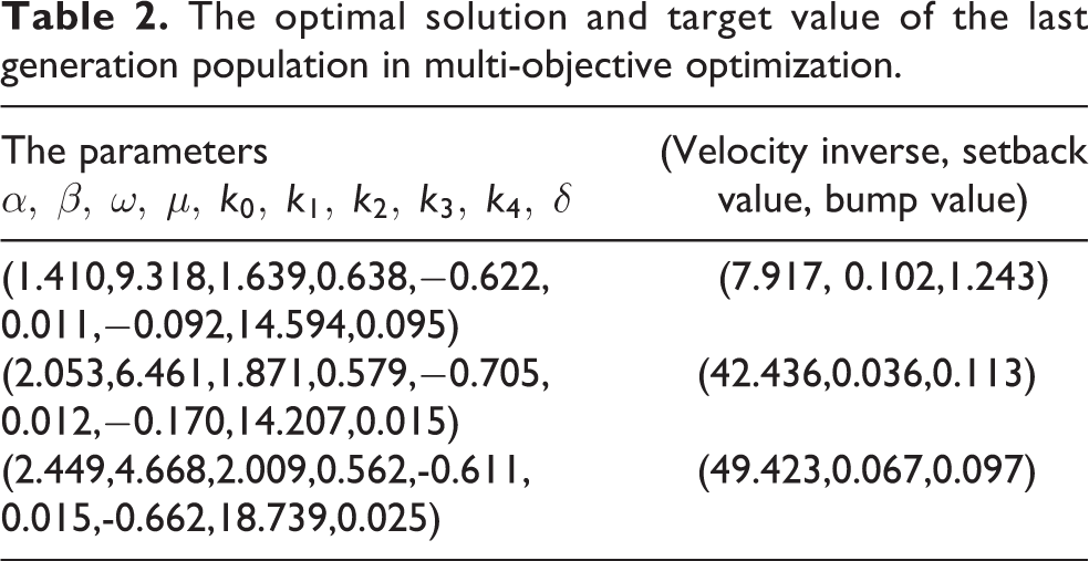
As shown above, the model parameters are optimized. The optimal solution and target value of the last generation population are shown in Table 2.
The optimal solution and target value of the last generation population in multi-objective optimization.
Experiment
Introduction of experimental prototype
The experimental platform adds a data acquisition device based on the original research. 26 As shown in Figure 11, the power of the experimental prototype is provided by an 8.4 V and 20 A switching power supply. The main controller communicates with the host computer through the wireless serial port module. In the experiment, the motion performance parameters of the robot are needed to obtain, which are the velocity, the setback degree, and the bump degree. The velocity is measured by a distance sensor between the experimental platform and the front board in the process of moving forward, and then the distance is divided by time. The distance sensor is installed in the front of the experimental platform, pointing to the direction of motion. The sampling time of distance and acceleration is 100 ms.

Experimental prototype.
The installation of the sensor is consistent with the center of the mass coordinate system of the experimental platform. The x-axis direction is parallel to the forward direction of the experimental platform, the z-axis dire perpendicular to the horizontal direction, and the y-axis is determined by the right-hand rule.
The data acquisition board is the ALLENTEK MiniSTM32 V3.3 development board. The laser sensor TF Mini communicates with the acquisition board through a serial port protocol. The accelerometer MPU6050 communicates with the acquisition board through TTL level serial port protocol. The acquisition board writes the data from a sensor to the SD card.
The experiment needs to run the results of the optimization algorithm on the experiment platform. The optimization result includes the values of CPG parameters. These values also need to be solved by the differential equations and mapped from the function to obtain joint angles that the servo motors can perform. Taking into account the poor solution ability on the single chip, these equations require a lot of CPU and memory resources. Therefore, after running the parameter results on PC to obtain joint angle values, we saved these results to the servo control board and then the servo control board output the motion command of these angle values.
Analysis of experimental results
The velocity used in the experiment is based on the displacement of the experimental platform measured by the displacement sensor, which is the difference of displacement. The displacement is obtained by moving the experimental platform within sampling time. In this experiment, the sampling time is 100 ms.
The data sampled during movement have noise. And a filter is needed firstly for removing the noise. The bump value is the vertical acceleration minus the gravity acceleration. The sensor gravity acceleration measured in the experiment is 0.92 m/s2.
In the simulation, the optimal individuals in the multi-objective optimization method among the three objectives are obtained, respectively. The three sets of parameters we obtain from the solution set
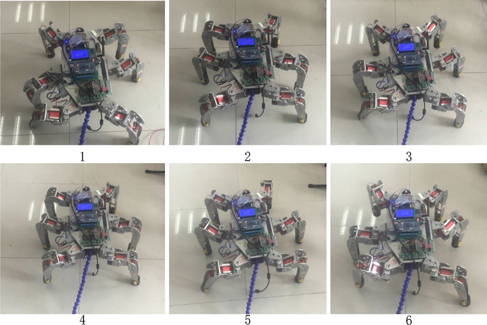
Motion decomposition diagram at optimal velocity.

Experimental results of optimal velocity. (a) Velocity smooth; (b) setback smooth; (c) bump smooth.
Taking the average values of data, we obtained the velocity, setback, and bump values as 0.072 m/s, 0.231 m/s2, and 1.645 m/s2, respectively.
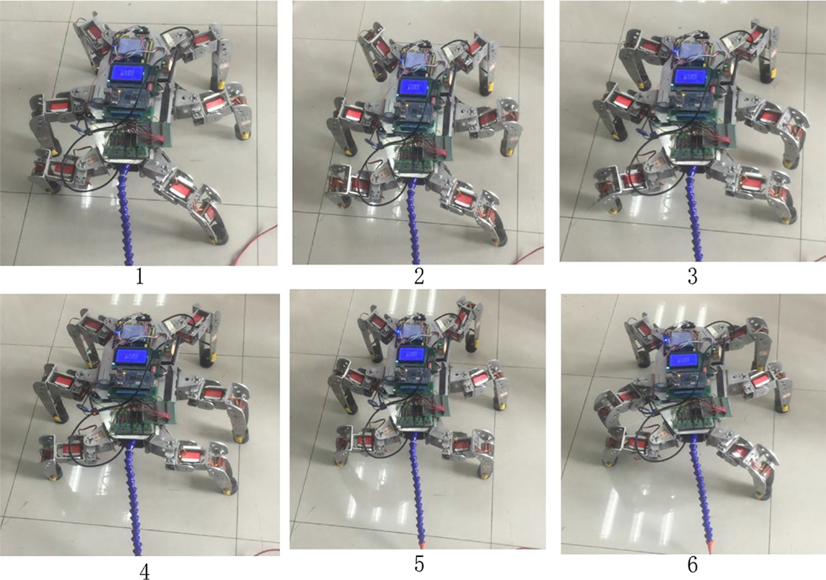
The motion decomposition in the optimal case of setback is shown in Figure 14. Figure 15 shows the data of setback, obtained in the optimal situation.
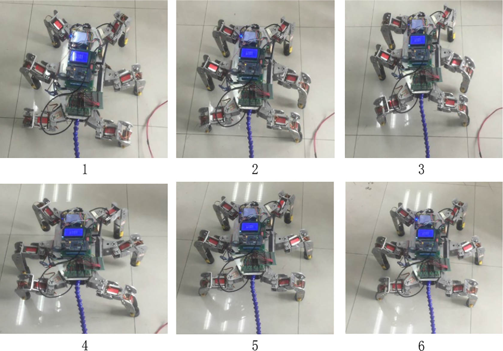
Motion decomposition diagram at optimal setback.

Experimental results of optimal setback. (a) Velocity smooth; (b) setback smooth; (c) bump smooth.
If taking the averaged values of the data, we can get the velocity, setback, and bump values as 0.027 m/s, 0.063 m/s2, and 0.275 m/s2, respectively.
The optimal motion decomposition of the bump is shown in Figure 16. The optimal bump motion pattern is shown in Figure 17.
Motion decomposition diagram at optimal bump.

Experimental results of optimal bump. (a) Velocity smooth; (b) setback smooth; (c) bump smooth.
If taking the averaged values of the measured data, we also get the velocity, setback, and bump values as 0.011 m/s, 0.104 m/s2, 0.213 m/s2, respectively.
The result of the simulation is the inverse of the velocity, which can be compared with the experimental results only after the velocity value is changed. The averaged values of the data above are also compared with the simulation results, as shown in Table 3.
Comparison between simulation and experiment.

The velocity values in the experiment reached 40.11% in simulation, and the setback value is 68.57% higher than that in simulation. The bump value is 156.43% higher than that in simulation. The shake of the experimental prototype in a vertical direction leads that the bump index is much different from simulation.
Conclusion
This article uses the CPG symmetric network consists of six Hopf oscillators. The angle values of the knee joint, hip joint, and ankle joint are obtained by the state value output of the CPG through the mapping functions. The multi-objective genetic algorithm is shown for optimizing the parameters of CPG, which schedules the movement of the hexapod robot.
In addition, we compare the experimental results of the multi-objective genetic algorithm and the single-objective genetic algorithm. We obtained the velocity target is not improved significantly, but the two goals of the setback value and the bump value are better than the single-objective genetic algorithm. Finally, the simulation results are verified by the experiment.
Supplemental material
Supplemental Material, sj-pdf-1-arx-10.1177_17298814211044934 - Parameters optimization of central pattern generators for hexapod robot based on multi-objective genetic algorithm
Supplemental Material, sj-pdf-1-arx-10.1177_17298814211044934 for Parameters optimization of central pattern generators for hexapod robot based on multi-objective genetic algorithm by Binrui Wang, Xiaohong Cui, Jianbo Sun and Yanfeng Gao in International Journal of Advanced Robotic Systems
Footnotes
Declaration of conflicting interests
The author(s) declared no potential conflicts of interest with respect to the research, authorship, and/or publication of this article.
Funding
The author(s) disclosed receipt of the following financial support for the research, authorship, and/or publication of this article: The authors would like to thank the National Natural Science Foundation of China under Grant (61903351). This work was also supported by National Key Technologies Research & Development Program of China (2018Y FB2101004).
Supplemental material
Supplemental material for this article is available online.
References
Supplementary Material
Please find the following supplemental material available below.
For Open Access articles published under a Creative Commons License, all supplemental material carries the same license as the article it is associated with.
For non-Open Access articles published, all supplemental material carries a non-exclusive license, and permission requests for re-use of supplemental material or any part of supplemental material shall be sent directly to the copyright owner as specified in the copyright notice associated with the article.