Air-breathing hypersonic vehicle trajectory optimization with uncertain no-fly zones

Abstract

The air-breathing hypersonic planes are considered to be the future of commercial airlines, which can fly from NYC to London in under an hour. For air-breathing vehicles, 3D trajectory planning will become extremely important due to its significant impact on flight performance. Past research on this issue was not comprehensive enough. Thus, we proposed a hybrid method for generating the optimal trajectories efficiently. No-fly zones are specified for geopolitical restrictions in air-breathing hypersonic vehicle missions. However, previous studies focused on no-fly zone constraints with fixed locations and boundaries. For robust execution, we must take into account no-fly zones’ uncertainties, which arise due to uncertain localization, measurement errors, and no-fly zones’ movement. A chance-constrained approach is presented here to deal with such uncertainties. The key idea of this method is controlling risk when the flight path is close to the uncertain no-fly zones. First, the trajectory planning of air-breathing hypersonic vehicles is modeled as a chance-constrained optimization (CCOPT) problem. With the help of the convexification and linearization techniques, we can approximate the non 3.2.2 CCOPT problem as a convex second-order cone programing under the Gaussian distribution assumption. It can be solved to global optimality by the interior point method. Finally, we give numerical simulation results to prove the effectiveness of this method.

Introduction

Trajectory planning for hypersonic vehicles such as an air-breathing hypersonic vehicle (ABHV) has received a great deal of attention in recent years.^1–4 An ABHV needs to be able to plan trajectories that take the vehicle from its current location to a goal while avoiding no-fly zones (NFZs). These trajectories should be optimal with respect to a criterion such as time or fuel consumption. This problem has two main challenges: First, the trajectory optimization problem of ABHV is highly complicated and inherently nonconvex. Second, there are a number of sources of uncertainty of no-fly zones, such as uncertain localization, measurement errors, and NFZs’ movement. Such uncertainty must be modeled as a form that can be processed by numerical algorithms to achieve robustness.

Many methods can be used to solve the problem of unpowered hypersonic gliding vehicle (HGV) trajectory planning. Model predictive programing, ⁵ pseudospectral method,^1,4,6 indirect method, ⁷ and convex optimization ⁸ all demonstrate their unique advantages in certain scenarios. Considering the need to generate trajectories quickly in some tasks, we proposed an algorithm based on geometric stitching. ⁹

As an application of heuristics algorithm, particle swarm optimization ¹⁰ and gravitational search algorithm ¹¹ can also give appropriate solutions. Furthermore, with the development of machine learning, deep neural networks have been used in HGV’s trajectory planning.^12,13

However, ABHV’s dynamic is much more complex. Its scramjet engine’s performance is highly correlated with the vehicle’s altitude, velocity, angle of attack, and throttle (as shown in equation (8)). As a result, the optimization algorithm is required to solve a multi-variable, highly non-linear and complex coupling problem in a limited time. Those methods developed for the unpowered vehicle are unsuitable and computationally expensive in this situation. Some existing work circumvents this problem using relatively simple propulsion system models.^14,15

In this work, we build a hybrid algorithm for ABHV with complex propulsion-pneumatic coupling based on convex optimization, ⁸ which has shown great application potential in recent years because of its serval superior features: ¹⁶ Every local minimum is a global minimum; if the objective function is strictly convex, then the problem has at most one optimal point. Some kinds of convex problems, like the second-order cone programing (SOCP), can be solved efficiently by primal-dual interior-point methods (IPMs) that only have polynomial complexity.

Previous work focuses on the no-fly zone with precisely known locations and boundaries, ⁸ which is modeled as a cylinder with its center at the specified longitude and latitude and a given radius. However, they do not explicitly take into account uncertainty, which arises for two reasons. First, the location and boundaries are not usually known exactly but are estimated using a statistical model, satellite imagery, or inaccurate intelligence analysis. Second, some NFZs can move even during the flight of ABHV. So in practice, the vehicle may collide with the real NFZ even if the planned trajectory did not. In this paper, we will address this issue.

There are two solutions. A feasible idea is to ensure that the aircraft will not enter NFZ even in the worst case, which leads to a conservative solution. Let NFZ_R be the real NFZ, and NFZ_P be the areas that NFZ_R may exist. The conservative solution asks the ABHV to bypass the NFZ_P even if NFZ_P is much larger than NFZ_R. It is a bad idea because of three reasons. First, it is a huge waste of aircraft performance. Second, ABHV’s maneuverability and flight range are limited. Bypassing such a large NFZ_P may cause mission failure. Not to mention the possibility that a NFZ_P happens to block the way to target. Flying through the NFZ_P is inevitable in this case. Third, ABHV’s performance is highly influenced by the flight conditions, and bypassing will make the vehicle deviate from the designed optimistic conditions.

Another solution is to tolerate some degree of risk if the probability of failure is below a specified threshold. Therefore, it is reasonable to demand constraint satisfaction with some level of probability of success. This calls for the use of chance constraints. Chance constraints ensure that the decision made by a model leads to a certain probability of complying with constraints. In the chance-constrained optimization (CCOPT), there exist inequality constraints that are formulated as $\mathrm{Prob}\{a_1\le x\le a_2\}\ge b$ , where a₁, a₂, b are constant, $x$ is the state and $\mathrm{Prob}\in [0,1]$ is the probability level. The chance constraints were first introduced by Charnes et al. ¹⁷ in 1958 to solve optimization problems under uncertainty. Since then, many studies from Prékopa, ¹⁸ Charnes and Cooper, ¹⁹ Li et al. ²⁰ have looked into more methods of analyzing CCOPT and using CCOPT to solve engineering problems. Blackmore et al. ²¹ and Ono et al. ²² brought this concept into the field of dynamic trajectory planning and proved its value in a variety of missions, like UAV and Mars landing, etc. Their work inspired us to use a similar technique in uncertain NFZ problems.

This paper focuses on solving ABHV’s trajectory planning problem with uncertain NFZ constraints. The rest of this article is organized as follows. Section 2 proposed the major problem of ABHV’s trajectory planning. Section 3 gives a unique hybrid method for ABHV’s trajectory planning that balances efficiency and accuracy. The convexification of chance-constrained NFZ is presented in Section 4. Section 5 presents the numerical simulation results of our methods. This paper concludes with Section 6 by providing a summary, some comments, and pointing some future research directions.

Problem statement

A highly coupled multi constraints aircraft model for integrated flight/propulsion

In this section, we describe the generic trajectory optimization problem for the cruising phase of the airbreathing hypersonic vehicle. Due to the flight/propulsion are highly coupled, the original problem must be formulated in a certain way conducive to the SOCP approach.

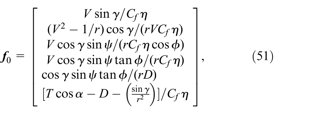
Regardless of the Earth rotation, a 3-DOF point-mass translation equations of motion of the ABHV with respect to non-dimensional time $\tau$ can be described as

$$\stackrel{·}{r}=V\sin \gamma$$

(1)

$$\stackrel{·}{\gamma }=[L\cos \sigma +T\sin \alpha \cos \sigma +F_{\mathrm{Ty}}\cos \alpha \cos \sigma +(V^2-1/r)\cos \gamma /r]/V$$

(2)

$$\stackrel{·}{\theta }=V\cos \gamma \sin \psi /(r\cos \varphi )$$

(3)

$$\stackrel{·}{\varphi }=V\cos \gamma \cos \psi /r$$

(4)

$$\stackrel{·}{\psi }=[(L\sin \sigma +T\sin \alpha \sin \sigma +F_{\mathrm{Ty}}\cos \alpha \sin \sigma )/\cos \gamma +V^2\cos \gamma \sin \psi \tan \varphi /r]/V$$

(5)

$$\stackrel{·}{V}=T\cos \alpha -D-\sin \gamma /r^2$$

(6)

$$\stackrel{·}{m}=-C_f(\mathrm{Mach},\alpha ,r)\eta$$

(7)

where $r$ is the radial distance from the Earth center to the vehicle; $\theta$ and $\varphi$ are the longitude and latitude, respectively; $\gamma$ is the flight-path angle of the Earth-relative velocity vector; $\psi$ is the heading angle, which is measured clockwise in the local horizontal plane from the north. $V$ donates the velocity of ABHV. All these variables are non-dimensional: the velocity is normalized by $\sqrt{g_0{R}_0}$ , where $g_0=9.81m/s^2$ and the Earth radius is $R_0=6378.135\mathrm{km}$ . The length is scaled by $R_0$ and time $\tau$ is normalized by $\sqrt{R_0/g_0}$ . $F_{\mathrm{Ty}}$ is the additional normal force caused by the scramjet engine. ²³ Let $L$ be the non-dimensional lift acceleration in $g_0$ , $D$ be the non-dimensional drag acceleration, and $T$ be the non-dimensional thrust acceleration. They are given by

$$\begin{array}{c}T=0.5R_0\rho V^2{S}_{\mathrm{Engine}}{C}_T(\mathrm{Mach},\alpha ,\eta ,r)/m\hfill \\ L=0.5R_0\rho V^2{S}_{\mathrm{Ref}}{C}_L(\mathrm{Mach},\alpha ,r)/m\hfill \\ D=0.5R_0\rho V^2{S}_{\mathrm{Ref}}{C}_D(\mathrm{Mach},\alpha ,r)/m\hfill \end{array}$$

(8)

where $\rho$ is the local atmosphere density. $C_L$ , $C_D$ , and $C_T$ correspond to the lift, drag, and thrust coefficient, respectively. They are functions of Mach number, angle of attack $\alpha$ , non-dimensional throttle $\eta$ , and altitude $r$ . $S_{\mathrm{ref}}$ and $m$ are the reference area and mass of the vehicle, respectively. $S_{\mathrm{Engine}}$ is the reference area of the scramjet engine. $C_f(\mathrm{Mach},\alpha ,r)$ is the fuel consumption rate.

State and control constraints

The control inputs $\sigma$ and $\alpha$ respectively donates the bank angle and angle of attack. Their saturation limitation can be presented by following equations

$${\alpha }_{min}\le \alpha \le {\alpha }_{max}$$

(9)

$$|\sigma |\le {\sigma }_{max}$$

(10)

The throttle is also limited

$${\eta }_{min}\le \eta \le {\eta }_{max}$$

(11)

We use ${\mathit{u}}_0=[\alpha \cos \sigma \sin \sigma \eta ]$ to replace the $[\alpha \sigma \eta ]$ in equations (1)–(8). It is because Liu et al., ²⁷ and Zhao and Song ²⁴ pointed out that directly using $\sigma$ as a control variable introduces significant high-frequency chatters, which is generally detrimental to the convergence of the successive solution process. Obviously, the new control input $\mathit{u}$ must satisfy equation (12).

$${\mathit{u}}_0(2{)}^2+{\mathit{u}}_0(3{)}^2=1$$

(12)

For an HGV, the total potential energy is monotonically decreasing during the gliding process because of drag, so an energy-like variable is used as the independent variable of the programing. ²⁷ However, when it comes to an ABHV with scramjet, it is not suitable. As a result, we need to find a new independent variable. In all states in the equations (1)–(7), time $\tau$ and mass $m$ are monotonical during the flight. In this paper, we prefer mass to time as the independent variable due to the following reason:

1. The dynamic equations (1)–(7) can be reduced to 6 dimensions from 7 dimensions.

2. If we choose time as the independent variable and the terminal time is unavailable, it is hard to define the terminal constraints of the problem. In contrast, terminal mass is easy to be given in a maximum-downrange problem.

$m$ is decreasing during the flight, so let the increasing variable $\tilde{m}=-m$ be the new independent variable.

Let $\mathit{x}=[r\gamma \theta \varphi \psi V]$ , then

$$d\mathit{x}/d\tilde{m}=\frac{d\mathit{x}}{d\tau }\times \frac{d\tau }{d\tilde{m}}=\frac{1}{C_f\eta }\frac{d\mathit{x}}{d\tau }$$

(13)

Substitute equation (13) into equations (1)–(7), we obtain

$$\mathrm{dr}/d\tilde{m}=V\sin \gamma /C_f\eta$$

(14)

$$\begin{array}{c}d\gamma /d\tilde{m}\hfill \\ =[L\cos \sigma +T\sin \alpha \cos \sigma +F_{\mathrm{Ty}}\cos \alpha \cos \sigma +(V^2-1/r)\cos \gamma /r]\hfill \\ /(V{C}_f\eta )\hfill \end{array}$$

(15)

$$d\theta /d\tilde{m}=V\cos \gamma \sin \psi /(r{C}_f\eta \cos \varphi )$$

(16)

$$d\varphi /d\tilde{m}=V\cos \gamma \cos \psi /(r{C}_f\eta )$$

(17)

$$d\psi /d\tilde{m}=[(L\sin \sigma +T\sin \alpha \sin \sigma +F_{\mathrm{Ty}}\cos \alpha \sin \sigma )/\cos \gamma +V^2\cos \gamma \sin \psi \tan \varphi /r]/(V{C}_f\eta )$$

(18)

$$\mathrm{dV}/d\tilde{m}=[T\cos \alpha -D-\left(\frac{\sin \gamma }{r^2}\right)]/C_f\eta$$

(19)

Thus the inequality constraints on controls that derived from equations (9)–(12), are given as

$$\mathit{C}({\mathit{u}}_0,\tilde{m})\le 0$$

(20)

The initial and terminal constraints are described respectively by

$$\mathit{x}({\tilde{m}}_0)-{\mathit{x}}_0=0\Rightarrow \mathit{H}(\mathit{x}({\tilde{m}}_0),{\mathit{x}}_0)=0$$

(21)

$$\mathit{x}({\tilde{m}}_f)-{\mathit{x}}_f=0\Rightarrow \mathit{\Psi }(\mathit{x}({\tilde{m}}_f),{\mathit{x}}_f)=0$$

(22)

where ${\tilde{m}}_0$ and ${\tilde{m}}_f$ correspond to the initial and terminal $\tilde{m}$ of the vehicle, respectively.

Path and NFZ chance constraints

The heating rate $\stackrel{·}{Q}$ , dynamic pressure $q$ , and normal load $n$ are also constrained:

$$\stackrel{·}{Q}=k_Q\sqrt{\rho }{\sqrt{g_0{R}_0}}^{3.15}{V}^{3.15}\le {\stackrel{·}{Q}}_{\max }$$

(23)

$$q=0.5\rho g_0{R}_0{V}^2\le q_{\max }$$

(24)

$$n=\sqrt{L^2+D^2}\le n_{\max }$$

(25)

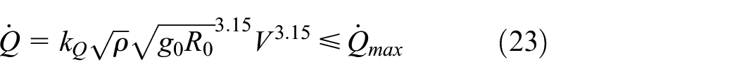
Equations (23)–(25) can also be expressed as altitude constraints because all of them are functions of $r$ and $V$ .

$$r\ge max(r_{\stackrel{·}{Q}}(r,V),r_q(r,V),r_n(r,V))$$

(26)

which can also be written as

$$r(\tilde{m})\ge max(r_{\stackrel{·}{Q}}(\tilde{m}),r_q(\tilde{m}),r_n(\tilde{m}))=r_{\min }(\tilde{m})$$

(27)

corresponding to different $\tilde{m}$ .

Meanwhile, to avoid flying too high, the upper boundary is given by

$$r(\tilde{m})\le r_{max}$$

(28)

Thus,

$$r_{\min }(\tilde{m})\le r(\tilde{m})\le r_{max}$$

(29)

Besides, the velocity of ABHV is also constrained

$$V_{min}\le V(\tilde{m})\le V_{max}$$

(30)

Equations (26), (29), and (30) yields the normalized path constraints:

$$\mathit{Path}(\mathit{x},\mathit{u},\tilde{m})=\left[\begin{array}{c}\mathit{Pat}{\mathit{h}}_{\stackrel{·}{Q}}\hfill \\ \multicolumn{1}{c}{\mathit{Pat}{\mathit{h}}_q}\\ \multicolumn{1}{c}{\mathit{Pat}{\mathit{h}}_n}\\ \multicolumn{1}{c}{\mathit{Pat}{\mathit{h}}_V}\end{array}\right]\le 0$$

(31)

An NFZ is an area over which aircraft are not permitted to fly. NFZs may be established for safety, environmental protection, or other reasons. In previous works, the determined NFZs are modeled as no-fly cylinders with given radii and center coordinates:

$$(\theta -{\theta }_{\mathrm{NFZ}}{)}^2+(\varphi -{\varphi }_{\mathrm{NFZ}}{)}^2\ge r_{\mathrm{NFZ}}^2$$

(32)

where ${\theta }_{\mathrm{NFZ}}$ and ${\varphi }_{\mathrm{NFZ}}$ are the center coordinates of the NFZs and $r_{\mathrm{NFZ}}$ is the radius.

When it comes to uncertainty, things have changed. Due to the initial estimation error or the movement of NFZ_R, the real NFZ_R may appear anywhere in a certain area NFZ_P (As shown in Figure 1). When it becomes inevitable to cross this NFZ_P, a very natural idea is to turn the original hard NFZ constraint into a soft one: Reducing the risk of passing through the NFZ_R (which means mission failed) to a certain level. Then we have the following optimization goal: completing the original task based on satisfying the specific probability of success requirement. In this paper, a chance constraint is used to describe the probability of success requirement, which can be derived from the preceding hard NFZ constraint (32):

$$\mathit{P}(\mathit{x},\tilde{m})=\mathrm{Pr}\{(\theta -{\theta }_{\mathrm{NFZ}}{)}^2+(\varphi -{\varphi }_{\mathrm{NFZ}}{)}^2\ge r_{\mathrm{NFZ}}^2\}\ge P*$$

(33)

Figure 1.

Uncertain NFZ.

where $\mathrm{Pr}\mathbf{\{}\mathrm{A}\mathbf{\}}$ is the probability of an event A, $P*$ is the probability of success threshold, which means that the probability of not-colliding with the NFZ_R must be greater than or equal to $P*$ . Thus, the original problem turns into a CCOPT problem. In past research, the CCOPT problem can be solved in a variety of ways, such as the Monte Carlo method, particle swarm method, etc. But most of them are too slow to be used for an online algorithm. For the sake of computation efficiency, we propose an analytic approximation strategy as described in Section 3, which has been proven to be effective and highly efficient.

ABHV trajectory planning problem with uncertain NFZs

The optimal trajectory planning problem of ABHV with uncertain NFZs is formulated as the following optimal control problem.

$$\mathrm{P}0:\mathrm{minimize}\mathit{J}$$

(34)

$$\mathrm{subject}\mathrm{to}\stackrel{·}{\mathit{x}}=\mathit{f}(\mathit{x},{\mathit{u}}_0,\tilde{m})$$

(35)

$$\mathit{H}(x({\tilde{m}}_0),x_0)=0,\mathit{\Psi }(x({\tilde{m}}_f),x_f)=0$$

(36)

$$\mathbf{P}\mathit{ath}(\mathit{x},{\mathit{u}}_0,\tilde{m})\le 0,\mathit{C}({\mathit{u}}_0,\tilde{m})\le 0$$

(37)

$$\mathit{P}(\mathit{x},\tilde{m})\ge P*$$

(38)

The details of the performance index $\mathit{J}$ will be discussed in Section 3.2.

Trajectory optimization for air-breathing hypersonic vehicle

Considering the lack of a widely recognized ABHV trajectory optimization method so far, this article first proposes a SOCP-based hybrid trajectory planning algorithm before introducing uncertain NFZ.

A typical SOCP has the following form

$$\begin{array}{c}\min c^{T}x\hfill \\ \mathrm{subject}\mathrm{to}{a}_i^{T}x=b_i,i=1,\dots ,p\hfill \\ \Vert G_{i}x+g_i\Vert \le d_i^{T}x+e_i,i=1,\dots ,m\hfill \end{array}$$

(39)

where $x\in {\mathbb{R}}^n$ is the variable to be optimized $c\in {\mathbb{R}}^n$ $a_i\in {\mathbb{R}}^n$ $b_i\in \mathbb{R}$ $G_i\in {\mathbb{R}}^{(n_i-1)\times n}$ $g_i\in {\mathbb{R}}^{n_i-1}$ $d_i\in {\mathbb{R}}^n$ , $e_i\in \mathbb{R}$ . The inequality $\Vert G_{i}x+g_i\Vert \le d_i^{T}x+e_i$ is called second-order cone constraint and its dimension is $n_i$ .

P0 in Section 2.4 contains highly nonlinear dynamics, nonlinear path constraints, and nonconvex control constraints that cannot be directly solved with the framework of SOCP. Blackmore and Liu^25–27 introduced lossless convexification techniques and relaxation methodology that convert the original aerospace problem into the specific form required in SOCP. In this chapter, similar techniques are used. Of course, the existing framework ²⁷ needs to be further modified to accommodate the specificity of the air-breathing vehicle problem.

Furthermore, a hybrid method that combines online and offline computing is proposed to balance computational complexity and accuracy.

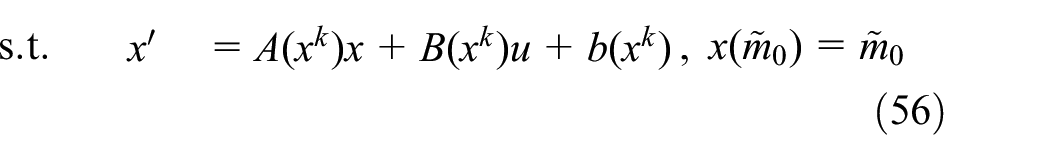
A hybrid method

P0 contains a four-dimensional control input vector ${\mathit{u}}_0=[\alpha \cos \sigma \sin \sigma \eta ]$ , and the elements in this vector are coupled with each other, as shown in equations (15)–(18).

Solving such a complex optimal control problem in a given time is challenging. To reduce the difficulty of computation and improve efficiency, a hybrid method is introduced:

We hope ABHV can reach the maximum range if needed, which can be approximated in a discretized form

$$\begin{array}{c}s\approx \sum _{i=1}^n{V}_i\mathrm{\Delta }{\tau }_i=\sum _{i=1}^n{V}_i\frac{\mathrm{\Delta }{m}_i}{{\stackrel{·}{m}}_i}=(m_f-m_0)\sum _{i=1}^n\frac{V_i}{{\stackrel{·}{m}}_i}\hfill \\ =(m_0-m_f)\sum _{i=1}^n\frac{V_i}{C_f(\mathrm{Mac}{h}_i,{\alpha }_i,r_i){\eta }_i}\hfill \end{array}$$

(40)

where $s$ is flight range, and ${\tau }_{\mathrm{togo}}$ is time-to-go. The entire flight process is divided into n-1 parts and i represents the i-th discrete point. $\mathrm{\Delta }{m}_i$ is the mass change between each discrete point. Equation (40) reveals that for a given fuel consumption, maximizing the total range is equivalent to maximizing the indicator $V_i/C_f(Mac{h}_i,{\alpha }_i,r_i){\eta }_i$ at each discrete point. Since $\alpha$ and $\eta$ directly affects this indicator in the cruising phase, it is reasonable to give them higher calculation priority than $\cos \sigma$ and $\sin \sigma$ . Besides, if we solve $\alpha$ and $\eta$ first, the control input of the original problem will be decoupled, and the quantity of computation will be significantly reduced. According to the above ideas, a hybrid method is obtained (Table 1). First, in the offline part, the optimal $\alpha$ and $\eta$ combination in the whole flight envelope is solved offline. Then, the actual optimal control problem is solved online.

Table 1.

The procedure of the hybrid method.

Offline part:

(a) Divide the flight envelope into n points with different velocities, altitudes, and masses. {(V1, r1, m1), (V2, r2, m2), …, (Vn, rn, mn)}. (b) Choose a state point (Vi, ri, mi), assume that the vehicle satisfies the quasi-steady level flight conditions ( $\sigma =0$ ) at this point $\gamma \prime \approx 0$ (41) and we want to maximize the $\frac{V_i}{C_f(\mathrm{Mac}{h}_i,{\alpha }_i,r_i){\eta }_i}$ . This is a static optimization problem that can be easily solved by mature algorithms such as the trust-region reflection method. The result is the optimal combination $({\alpha }_i,{\eta }_i)*$ that guarantees the maximum range capability. (c) save state and $({\alpha }_i,{\eta }_i)*$ in a mapping table, choose another state point, go back to b) until traverse all the points.

Online part:

(a) Discretize the state equation of the optimal control problem. Generate an initial trajectory guess ${\mathit{x}}^0$ at the beginning of the iteration. (b) At each discrete point we calculate the (V, r, m) along the initial trajectory, then the $(\alpha ,\eta )$ command can be achieved by interpolation from the mapping table. Substitute $(\alpha ,\eta )$ into state equation. As a result, the only unknown variable that exists in the state equation is $[\cos \sigma \sin \sigma ]$ . Solve the problem using the convex optimization method like the SOCP described in Section 3.5. (c) Update the initial trajectory with the result ${\mathit{x}}^1$ , go back to b), repeat the above process until we find an ${\mathit{x}}^k(k=0,1,2,\dots )$ which fully meets the optimization goal.

Multi-objective optimization performance index

Without loss of generality, the performance index or cost function of ABHV is given in following form in this paper:

$$\begin{array}{c}\mathrm{minimize}\mathit{J}={\kappa }_1{\mathit{J}}_1+{\kappa }_2{\mathit{J}}_2+{\kappa }_3{\mathit{J}}_3+\dots \hfill \\ ={\kappa }_1{\int }_{{\tilde{m}}_0}^{{\tilde{m}}_f}{\Gamma }_1(\mathit{x},\tilde{m})d\tilde{m}+{\kappa }_2{\int }_{{\tilde{m}}_0}^{{\tilde{m}}_f}{\Gamma }_2(\mathit{x},\tilde{m})d\tilde{m}+\dots \hfill \end{array}$$

(42)

where $\kappa$ is weight factor. In order to satisfy the form of SOCP, the performance index must be linear. Thus, the above equation must be reorganized before application.

Minimum terminal error

In the general trajectory planning problem, we hope that the vehicle will eventually reach a certain designated position. However, direct use of terminal constraint (22) is not good for algorithm convergence.

Thus, the terminal position constraints

$$\theta (\tilde{m})-{\theta }_f=0,\varphi (\tilde{m})-{\varphi }_f=0$$

(43)

are transformed into a performance index

$$\begin{array}{c}\mathrm{minimize}{\mathit{J}}_1={\kappa }_{11}\vartheta +{\kappa }_{12}\phi \hfill \\ \mathrm{subject}\mathrm{to}|\theta ({\tilde{m}}_f)-{\theta }_f|\le \vartheta \hfill \\ |\varphi (\tilde{m})-{\varphi }_f|\le \phi \hfill \end{array}$$

(44)

where $\kappa$ is weight factor.

Maximum flight range

In a real mission, straight&level flight ( $\sigma =0$ ) in the cruising phase probably does not keep the scramjet engine in the most efficient interval. In some cases, flying with a certain bank angle $\sigma$ $(\sigma \ne 0)$ may be a more sensible strategy. In addition, when ABHV has to circumvent obstacles like NFZs, we hope that the performance loss caused by bank angle $\sigma$ is minimal.

So, use the indicator $\frac{V_i}{C_{f_i}{\eta }_i}$ mentioned in section 3.1 to minimize the range loss

$${\mathit{J}}_2=\frac{1}{s}={\int }_{{\tilde{m}}_0}^{{\tilde{m}}_f}{C}_f\eta /Vd\tilde{m}=\sum _{{\tilde{m}}_0}^{{\tilde{m}}_f}(C_f\eta /V)$$

(45)

Equation (45) is noncovex, so it can be further expanded into a second-order Taylor series to fit the form requirement of SOCP as shown in Liu et al. ²⁷

Minimum time

The performance index with time is

$${\mathit{J}}_3={\int }_{{\tau }_0}^{{\tau }_f}1d\tau ={\int }_{{\tilde{m}}_0}^{{\tilde{m}}_f}(1/C_f\eta )d\tilde{m}$$

(46)

Equation (46) also can be expanded into a second-order Taylor series at each discrete point.

Convexification

Obviously, the problem P0 does not conform to the general SOCP form (39), so it still needs to be convexified and simplified. The process is given below.

Convexification of control constraints

As shown in Table 1, the only two control inputs that need to be handled are ${\mathit{u}}_0(2)=\cos \sigma$ and ${\mathit{u}}_0(3)=\sin \sigma$ . Let us redefine the control input $\mathit{u}=[\cos \sigma \sin \sigma ]$ . Liu et al. ²⁷ introduced an effective control constraint relaxation method for typical HGV, which is also suitable for the problem of this article. As the active assurances of the relaxed control constraints are already proved independently in Liu et al., ²⁷ the detailed proof is not presented here. As a result, the control constraint (12) is relaxed into the following form:

$$\mathit{u}(1{)}^2+\mathit{u}(2{)}^2\le 1$$

(47)

$$\cos {\sigma }_{max}\le \mathit{u}(1)\le \cos {\sigma }_{min}$$

(48)

Liu et al. ²⁷ assures that this condition will hold in the solution of the original problem. Obviously, the restructured constraint (47) is second-order cone and is suitable for SOCP.

Convexification of path constraints

In Section 2, the heating rate, dynamic pressure, and overload constraints, which are regarded as path constraints, were restructured into altitude constraint (26). The max function in $r(\tilde{m})\ge max(r_{\stackrel{·}{Q}}(\tilde{m}),r_q(\tilde{m}),r_n(\tilde{m}))$ is convex, so the discrete form (about ${\tilde{m}}_i$ ) is linear and convex

$$r({\tilde{m}}_i)\ge r_{min}({\tilde{m}}_i)$$

(49)

where ${\tilde{m}}_i$ corresponds to the i-th discrete point.

Linearization of dynamics

The nonlinear dynamics must be approximately linearized before applying the optimization algorithm. To improve the convergence and robustness of the algorithm, the computing process is designed as an iteration: A pre-designed linear trajectory is used as the initial guess reference trajectory at the first iteration, then the reference trajectory will be updated with the result of k-th iteration $\{\mathit{x}{(\tilde{m})}^k,\mathit{u}{(\tilde{m})}^k\}$ at the beginning of the k + 1th iteration. The pre-designed trajectory can be a linear trajectory and its feasibility does not affect the result.

Decouple the right side of equation (35) and rewrite it in a concise form ²⁵

$$\frac{d\mathit{x}}{d\tilde{m}}={\mathit{f}}_0(\mathit{x},\tilde{m})+\mathit{B}(\mathit{x},\tilde{m})\mathit{u}$$

(50)

where

$${\mathit{f}}_0=\left[\begin{array}{c}V\sin \gamma /C_f\eta \hfill \\ \multicolumn{1}{c}{(V^2-1/r)\cos \gamma /(\mathrm{rV}{C}_f\eta )}\\ \multicolumn{1}{c}{V\cos \gamma \sin \psi /(r{C}_f\eta \cos \varphi )}\\ \multicolumn{1}{c}{V\cos \gamma \sin \psi \tan \varphi /(r{C}_f\eta )}\\ \multicolumn{1}{c}{\begin{array}{c}\cos \gamma \sin \psi \tan \varphi /(\mathrm{rD})\hfill \\ \multicolumn{1}{c}{[T\cos \alpha -D-\left(\frac{\sin \gamma }{r^2}\right)]/C_f\eta }\end{array}}\end{array}\right],$$

(51)

$$B=\left[\begin{array}{cc}0\hfill & 0\hfill \\ \multicolumn{1}{c}{[L+T\sin \alpha +F_{\mathrm{Ty}}\cos \alpha ]/(V{C}_f\eta )}& 0\hfill \\ \multicolumn{1}{c}{0}& 0\hfill \\ \multicolumn{1}{c}{0}& 0\hfill \\ \multicolumn{1}{c}{\begin{array}{c}0\hfill \\ \multicolumn{1}{c}{0}\end{array}}& \begin{array}{c}[L+T\sin \alpha +F_{\mathrm{Ty}}\cos \alpha ]/(\cos \gamma V{C}_f\eta )\hfill \\ \multicolumn{1}{c}{0}\end{array}\hfill \end{array}\right]$$

(52)

In the offline part, the optimal $\alpha$ and $\eta$ combination have been already obtained. Thus, L, T, $F_{\mathrm{Ty}}$ , and D in equations (51) and (52) are determined only by the flight status $\mathit{x}$ .

To solve the dynamic problem, the equation (51) must be linearized. Let ${\mathit{x}}^k={\mathit{x}}^k(\tilde{m})$ and ${\mathit{u}}^k$ be the solution pair in k-th iteration. So at the (k + 1)-th iteration, linearizing of equation (51) yields ²⁷

$$\frac{d\mathit{x}}{d\tilde{m}}=\mathit{A}({\mathit{x}}^k){\mathit{x}}^k+\mathit{B}({\mathit{x}}^k){\mathit{u}}^k+\mathit{b}({\mathit{x}}^k)\mathit{x}({\tilde{m}}_0)={\mathit{x}}_0$$

(53)

where $\mathit{A}({\mathit{x}}^k)=\frac{\partial {\mathit{f}}_0({\mathit{x}}^k)}{\partial {\mathit{x}}^k}$ and $\mathit{b}({\mathit{x}}^k)={\mathit{f}}_0({\mathit{x}}^k)-\mathit{A}({\mathit{x}}^k){\mathit{x}}^k$ .

In order to ensure the reliability of linearization, a new constraint (54) including a trust-region column vector $\mathit{\delta }\in {\mathbb{R}}^6$ is added.

$$|x(\tilde{m})-x^k(\tilde{m})|\le \mathit{\delta }$$

(54)

As a result, P0 is transformed into P1 with given $(\alpha ,\eta )*$ that obtained in offline part.

$$\mathrm{P}1:\min \mathit{J}={\kappa }_1{\mathit{J}}_1+{\kappa }_2{\mathit{J}}_2+\dots$$

(55)

$$\mathrm{s}.\mathrm{t}.\begin{array}{cc}x\prime \hfill & =A(x^k)x+B(x^k)u+b(x^k)\hfill \end{array},x({\tilde{m}}_0)={\tilde{m}}_0$$

(56)

$$|x(\tilde{m})-x^k(\tilde{m})|\le \mathit{\delta }$$

(57)

$$u_1(\tilde{m}{)}^2+u_2(\tilde{m}{)}^2\le 1$$

(58)

$${\omega }_l\le u_1(\tilde{m})\le {\omega }_h$$

(59)

$$max(r_{min},r_{\stackrel{·}{Q}},r_{\overline{q}})\le r(\tilde{m})\le r_{max}$$

(60)

$$V_{min}\le V(\tilde{m})\le V_{max}$$

(61)

$$|\theta ({\tilde{m}}_f)-{\theta }_f|\le \vartheta ,|\varphi (\tilde{m})-{\varphi }_f|\le \phi$$

(62)

$$r({\tilde{m}}_f)=r_f\gamma ({\tilde{m}}_f)={\gamma }_f\psi ({\tilde{m}}_f)={\psi }_f$$

(63)

$$\mathit{P}(\mathit{x},\tilde{m})\ge P*$$

(64)

where $\kappa$ is the weight factor.

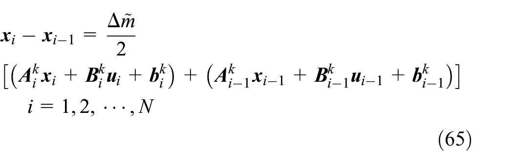
Discretization and the solution procedure of online part

In order to be solved by numerical algorithms, continuous systems in optimization problems are always discretized in practice. Of course, all the constraints must be satisfied at these discrete points. In this case, the independent variable is $\tilde{m}$ . So if we discretize equation (53) into N + 1 points equally, then the step size of $\tilde{m}$ is $\mathrm{\Delta }\tilde{m}={\tilde{m}}_i-{\tilde{m}}_{i-1}=({\tilde{m}}_N-{\tilde{m}}_0)/N$ . Hence, the states in problem P1 can be denoted as $\{\mathit{x}({\tilde{m}}_0),\mathit{x}({\tilde{m}}_1),\mathit{x}({\tilde{m}}_2),\cdots ,\mathit{x}({\tilde{m}}_N)\}$ , and similarly, the control can be denoted as $\{\mathit{u}({\tilde{m}}_0),\mathit{u}({\tilde{m}}_1),\mathit{u}({\tilde{m}}_2),\cdots ,\mathit{u}({\tilde{m}}_N)\}$ . Let ${\mathit{x}}_i=\mathit{x}({\tilde{m}}_i)$ and ${\mathit{u}}_i=\mathit{u}({\tilde{m}}_i)$ , the trapezoidal rule is applied to obtain the integral result from equation (53), which is given by

$$\begin{array}{c}{\mathit{x}}_i-{\mathit{x}}_{i-1}=\frac{\mathrm{\Delta }\tilde{m}}{2}\hfill \\ [({\mathit{A}}_i^k{\mathit{x}}_i{+\mathit{B}}_i^k{\mathit{u}}_i+{\mathit{b}}_i^k)+({\mathit{A}}_{i-1}^k{\mathit{x}}_{i-1}{+\mathit{B}}_{i-1}^k{\mathit{u}}_{i-1}+{\mathit{b}}_{i-1}^k)]\hfill \\ i=1,2,\cdots ,N\hfill \end{array}$$

(65)

where ${\mathit{A}}_i^k=\mathit{A}\left({\mathit{x}}^k\left({\tilde{m}}_i\right)\right)$ , ${\mathit{B}}_i^k=\mathit{B}\left({\mathit{x}}^k\left({\tilde{m}}_i\right)\right)$ , and ${\mathit{b}}_i^k=\mathit{b}\left({\mathit{x}}^k\left({\tilde{m}}_i\right)\right)$ . Equation (65) can be rearranged as

$$\begin{array}{c}{\mathit{H}}_{i-1}{\mathit{x}}_{i-1}-{\mathit{H}}_i{\mathit{x}}_i+{\mathit{G}}_{i-1}{\mathit{u}}_{i-1}+{\mathit{G}}_i{\mathit{u}}_i\hfill \\ =-\frac{\mathrm{\Delta }\tilde{m}}{2}({\mathit{b}}_i^k+{\mathit{b}}_{i-1}^k)i=1,2,\cdots ,N\hfill \end{array}$$

(66)

where ${\mathit{H}}_{i-1}=\mathit{I}+\frac{\mathrm{\Delta }\tilde{m}}{2}{\mathit{A}}_{i-1}^k$ , ${\mathit{H}}_i=\mathit{I}-\frac{\mathrm{\Delta }\tilde{m}}{2}{\mathit{A}}_i^k$ , ${\mathit{G}}_{i-1}=\frac{\mathrm{\Delta }\tilde{m}}{2}{\mathit{B}}_{i-1}^k$ , ${\mathit{G}}_i=\frac{\mathrm{\Delta }\tilde{m}}{2}{\mathit{B}}_i^k$ . $\mathit{I}$ is a unit matrix with the same dimension as that of $\mathit{A}$ .

By combining the state variable ${\mathit{x}}_i$ and control variable ${\mathit{u}}_i$ , together with the accessorial vector $\vartheta$ and $\phi$ (introduced in section 3.2.1), we can obtain the optimization variable vector $\mathit{z}$ :

$$\mathit{z}=[{\mathit{x}}_0^T\dots {\mathit{x}}_N^T{\mathit{u}}_0^T\dots {\mathit{u}}_N^T\vartheta \phi {]}^T$$

(67)

As a result, the whole discrete equation is given by

$$\mathit{Mz}=\mathit{F}$$

(68)

where

$$\mathit{M}=\left[\begin{array}{ccccccccccccc}\mathit{I}\hfill & 0\hfill & 0\hfill & 0\hfill & 0\hfill & 0\hfill & 0\hfill & 0\hfill & 0\hfill & 0\hfill & 0\hfill & 0\hfill & 0_{1\times 2}\hfill \\ \multicolumn{1}{c}{{\mathit{H}}_0}& {\mathit{H}}_1\hfill & 0\hfill & \dots \hfill & 0\hfill & 0\hfill & {\mathit{G}}_0\hfill & {\mathit{G}}_1\hfill & 0\hfill & \dots \hfill & 0\hfill & 0\hfill & 0_{1\times 2}\hfill \\ \multicolumn{1}{c}{⋮}& ⋮\hfill & ⋮\hfill & \ddots \hfill & ⋮\hfill & ⋮\hfill & ⋮\hfill & ⋮\hfill & ⋮\hfill & \ddots \hfill & ⋮\hfill & ⋮\hfill & ⋮\hfill \\ \multicolumn{1}{c}{0}& 0\hfill & 0\hfill & \dots \hfill & {\mathit{H}}_{N-1}\hfill & {\mathit{H}}_N\hfill & 0\hfill & 0\hfill & 0\hfill & \dots \hfill & {\mathit{G}}_{N-1}\hfill & {\mathit{G}}_N\hfill & 0_{1\times 2}\hfill \end{array}\right]$$

(69)

$$\mathit{F}=-\frac{\mathrm{\Delta }\tilde{m}}{2}\left[\begin{array}{c}-\frac{2}{\mathrm{\Delta }\tilde{m}}{\mathit{x}}_0\hfill \\ \multicolumn{1}{c}{{\mathit{b}}_1^k+{\mathit{b}}_0^k}\\ \multicolumn{1}{c}{⋮}\\ \multicolumn{1}{c}{{\mathit{b}}_N^k+{\mathit{b}}_{N-1}^k}\end{array}\right]$$

(70)

Obviously, the discretized constraints and performance index respectively illuminated from Section 3.2 through 3.3 are a linear function of $\mathit{z}$ . The performance index is denoted by ${\mathit{c}}^T\mathit{z}$ where $\mathit{c}$ is a constant vector. Thus, let ${\mathit{x}}_i=[r_i{\gamma }_i{\theta }_i{\varphi }_i{\psi }_i{V}_i{]}^T$ , a discretized version of problem P1 is given in the following:

$$\mathrm{P}2\mathrm{minimize}{\mathit{c}}^T\mathit{z}$$

(71)

$$\mathrm{s}.\mathrm{t}.\mathit{Mz}=\mathit{F}$$

(72)

$$|{{\mathit{x}}_i}^{k+1}-{{\mathit{x}}_i}^k|\le \mathit{\delta }$$

(73)

$${\mathit{u}}_i(1{)}^2+{\mathit{u}}_i(2{)}^2\le 1\cos {\sigma }_{max}\le {\mathit{u}}_i(1)\le \cos {\sigma }_{min}$$

(74)

$$r_{min}\le r_i\le r_{max}$$

(75)

$$V_{min}\le V_i\le V_{max}$$

(76)

$$|\theta (e_f)-{\theta }_f|\le \vartheta ,|\varphi (e_f)-{\varphi }_f|\le \phi$$

(77)

$$r({\tilde{m}}_N)=r_f\gamma ({\tilde{m}}_N)={\gamma }_f\psi ({\tilde{m}}_N)={\psi }_f$$

(78)

$$\mathit{P}(\mathit{x},\tilde{m})\ge P*$$

(79)

All of the constraints in P2 are either linear or second-order, and the performance index is linear, too. Therefore, the problem P2 is SOCP, which can be solved with primal-dual interior point method. Note that the dimension of $\mathit{M}$ is pretty large, directly depending on N. So superabundant discrete points will significantly depress the computational efficiency of the solution procedure. Although primal-dual interior point method shows its unique advantage in dealing with a large-scale sparse matrix like $\mathit{M}$ , N still needs to be chosen properly. The details of how to solve P2 are illustrated in Table 2.

Table 2.

Details of the iteration procedure of P2 in the online part.

(a) Set k = 0 and build an initial profile ${\mathit{x}}^0=\{{\mathit{x}}_0^0,{\mathit{x}}_1^0,{\mathit{x}}_2^0,\dots ,{\mathit{x}}_N^0\}$ . Just integrate the motion equation without control until the value of the flight-path angle changed from negative to positive for the first time. Let state at this time be ${\mathit{x}}_{\mathrm{initial}}^0$ and set zero bank angle, perform linear interpolation about $\tilde{m}$ between ${\mathit{x}}_{\mathrm{initial}}^0$ and ${\mathit{x}}_f^{*}$ . The result will be the initial profile. (b) At the (k + 1)th iteration (k ≥ 0), use ${\mathit{x}}^k$ to update those corresponding parameters in problem P2 (e.g. M and F in equation (72), ${\mathit{x}}_i^k$ in the trust-region constraint and $r_{min}^i$ in the path constraint). Then, solve problem P2 to get a solution ${\mathit{z}}^{k+1}$ . (c) Check if the solution meets the stopping criterion: $\underset{i}{max}(|{\mathit{x}}_i^{k+1}-{\mathit{x}}_i^k|)\le \mathbf{\epsilon }$ (81) If so, output the result. Otherwise, update ${\mathit{z}}^k$ with ${\mathit{z}}^{k+1}$ , set k = k + 1, and go back to (b).

According to several test results and Liu et al., ²⁷ the $\mathit{\delta }$ in equation (73) is select as:

$$\mathit{\delta }={\left[\frac{20000}{R_0}\frac{20\pi }{180}\frac{20\pi }{180}\frac{20\pi }{180}\frac{60\pi }{180}\frac{100}{\sqrt{g_0{R}_0}}\right]}^{\mathrm{T}}$$

(80)

Convexification of NFZ chance-constraints

Single NFZ chance-constraint

In Section 2.3, the uncertain NFZ is converted into a chance constraint optimization problem. These NFZ constraints are obviously concave so they cannot be substituted into the solving process directly. Whereas as shown in Liu et al., ²⁷ if the concave constraints are discounted, the concave constraints can be approximated successively by its linearized form, for example:

The hard NFZ constraint (32) is equal to

$$2({\theta }^{(k)}-{\theta }_{\mathrm{NFZ}})\theta +2({\varphi }^{(k)}-{\varphi }_{\mathrm{NFZ}})\varphi \ge d_{\mathrm{NFZ}}^2+{\overline{d}}_{\mathrm{NFZ}}$$

(82)

where ${\theta }^{(k)}$ and ${\varphi }^{(k)}$ are from kth iteration and

$$\begin{array}{c}{\overline{d}}_{\mathrm{NFZ}}=-({\theta }^{(k)}-{\theta }_{\mathrm{NFZ}}{)}^2-({\varphi }^{(k)}-{\varphi }_{\mathrm{NFZ}}{)}^2\hfill \\ +2({\theta }^{(k)}-{\theta }_{\mathrm{NFZ}})\theta +2({\varphi }^{(k)}-{\varphi }_{\mathrm{NFZ}})\varphi \hfill \end{array}$$

(83)

Similarly, the chance constraint is used to describe the probability of success requirement, which can be derived from the preceding linearized hard NFZ constraint (82):

$$\begin{array}{c}\mathrm{Eq}\left(33\right)\Rightarrow \mathrm{Pr}\{2({\theta }^{(k)}-{\theta }_{\mathrm{NFZ}})\theta \hfill \\ +2({\varphi }^{(k)}-{\varphi }_{\mathrm{NFZ}})\varphi \ge d_{\mathrm{NFZ}}^2+{\overline{d}}_{\mathrm{NFZ}}\}\ge P*\hfill \end{array}$$

(84)

Without loss of generality, the exact location of NFZ_R is unknown, so let the center coordinates be individual Gaussian-distribution uncertain parameters.

$${\theta }_{\mathrm{NFZ}}~\mathcal{N}({\overline{\theta }}_{\mathrm{NFZ}},{\Sigma }_{\theta \_\mathrm{NFZ}}){\varphi }_{\mathrm{NFZ}}~\mathcal{N}({\overline{\varphi }}_{\mathrm{NFZ}},{\Sigma }_{\varphi \_\mathrm{NFZ}})$$

(85)

where ${\overline{\theta }}_{\mathrm{NFZ}}$ and ${\overline{\varphi }}_{\mathrm{NFZ}}$ corresponds to the mean of longitude and latitude, respectively. $\Sigma$ represents the corresponding variances. Their value can be approximated using prior knowledge.

For the convenience of expression, let $\mathit{w}=[02({\theta }_{\mathrm{NFZ}}-{\theta }^{(k)})2({\varphi }_{\mathrm{NFZ}}-{\varphi }^{(k)})00{]}^T$ and $\varsigma =-(d_{\mathrm{NFZ}}^2+{\overline{d}}_{\mathrm{NFZ}})$ be the generalized uncertain parameter and determined parameter in equation (84), respectively. Obviously, $\mathit{w}$ obey Gaussian distribution

$$\mathit{w}~\mathcal{N}(\overline{\mathit{w}},{\Sigma }_{\mathrm{NFZ}})$$

(86)

where the corresponding variance ${\Sigma }_{\mathrm{NFZ}}=[2{\Sigma }_{\theta \_\mathrm{NFZ}}2{\Sigma }_{\varphi \_\mathrm{NFZ}}]$ , $\overline{\mathit{w}}$ is the mean of the new distribution.

Then equation (84) can be rewritten as

$$\mathrm{Pr}\{{\mathit{w}}^T\mathit{x}\le \varsigma \}\ge P*$$

(87)

Consider

$${\mathit{w}}^T\mathit{x}\le \varsigma ,\mathrm{with}\mathit{w}~\mathcal{N}(\overline{\mathit{w}},{\Sigma }_{\mathrm{NFZ}})$$

(88)

then

$${\mathit{w}}^T\mathit{x}-\varsigma \le 0~\mathcal{N}({\overline{\mathit{w}}}^T\mathit{x}-\varsigma ,{\mathit{x}}^T{\Sigma }_{\mathrm{NFZ}}\mathit{x})$$

(89)

hence

$$\mathrm{Pr}\{{\mathit{w}}^T\mathit{x}\le \varsigma \}=\mathrm{\Phi }\left(\frac{b-{\overline{\mathit{w}}}^T\mathit{x}}{\sqrt{{\mathit{x}}^T{\Sigma }_{\mathrm{NFZ}}\mathit{x}}}\right)$$

(90)

where $\mathrm{\Phi }$ is the Gauss cumulative distribution function and thus

$$\mathrm{Pr}\{{\mathit{w}}^T\mathit{x}\le \varsigma \}\ge P*\iff \varsigma -{\overline{\mathit{w}}}^T\mathit{x}\ge {\mathrm{\Phi }}^{-1}(P*)\Vert {{\Sigma }_{\mathrm{NFZ}}}^{1/2}\mathit{x}{\Vert }_2$$

(91)

which happens to be a second-order cone constraint for any $0.5\le P*\le 1$ (i.e. ${\mathrm{\Phi }}^{-1}(P*)\ge 0$ ). Hence, the chance constraint is converted into a hard boundary constraint. The inverse function ${\mathrm{\Phi }}^{-1}(P*)$ has no analytical form but can be calculated using a look-up method, or approximated as ²⁸

$${\mathrm{\Phi }}^{-1}(P*)=5.5556*(1-((1-P*)/P*{)}^{0.1186}$$

(92)

Note that if those uncertain parameters are not individual, it will become a much more challenging problem and requires more undiscovered skills to be solved.

Multiple NFZ chance-constraints

Let $Q$ be the number of NFZs. The multiple NFZ chance-constraint is given as

$$\mathrm{Pr}\{{{\mathit{w}}_j}^T\mathit{x}\le {\varsigma }_j,j=1,2,\dots ,Q\}\ge P*$$

(93)

where $j=1,2,\dots ,Q$ .

In order to apply the proposed analytic approximation method, we give the following relation

$$\begin{array}{c}\mathrm{Pr}\{{{\mathit{w}}_j}^T\mathit{x}\le {\varsigma }_j,j=1,2\dots \}=\mathrm{Pr}\{\underset{j\in 1,\dots ,Q}{\max }({{\mathit{w}}_j}^T\mathit{x}-{\varsigma }_j)\le 0\}\hfill \\ \ge \mathrm{Pr}\{\ln (\sum _{j=1}^Q[\exp ({{\mathit{w}}_j}^T\mathit{x}-{\varsigma }_j)])\le 0\}\hfill \end{array}$$

(94)

In fact, equation (94) follows from this generic inequality

$$max(x,y)\le \ln (e^x+e^y)$$

(95)

Consequently,

$$\mathrm{Pr}\{\ln (\sum _{\mathrm{j}=1}^{\mathrm{Q}}[\exp ({{\mathit{w}}_{\mathrm{j}}}^{\mathrm{T}}\mathit{x}-{\mathrm{\varsigma }}_{\mathrm{j}})])\le 0\}\ge P*$$

(96)

implies that

$$\mathrm{Pr}\{{{\mathit{w}}_j}^T\mathit{x}\le {\varsigma }_j,j=1,\dots ,Q\}\ge P*$$

(97)

So inequality (96) is stronger than constraint (93). If (96) holds, the trajectory must satisfy the multiple NFZ chance-constraints. Note that the log-sum-exp function in equation (96) is convex and the detailed proof can be found in book. ¹⁶ As a result, the multiple NFZ chance-constraints do not affect the convexity of the whole problem. To handle with (96), the log-sum-exp can be firstly linearized, then convert the result into a hard boundary with the technique in Section 3.6.1.

Numerical experiment

In this section, a series of numerical simulation demonstrations will be given to prove the effectiveness of the method described in this paper.

All these experiments are based on a generic research ABHV model called BABHV-1 (Figure 2), which is developed by Beihang University. It is a concept design for a 5-ton class reusable single-stage spaceplane, using a scramjet engine propulsion system. It has a tailless delta wing similar to SR-71. The purpose of this aircraft is to study the flight characteristics and control strategies of the air-breathing hypersonic vehicle at different speeds. Currently, a scaled model has been produced for the low-speed test flight. This design is capable of cruising at an altitude ranging from 24 to 32 km (Relative sea level) with a cruise Mach number of 5.0–7.5. As shown in Figures 3 and 4, the aerodynamic and thrust coefficients vary with flight conditions and throttle.

Figure 2.

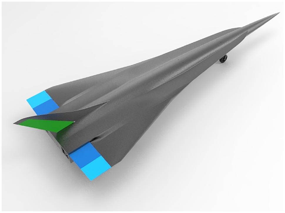
3D model and performance of BABHV-1.

Figure 3.

Thrust coefficient surface plot of BABHV-1.

Figure 4.

Lift coefficient surface plot of BABHV-1 ( $\alpha$  = 3 deg, $r$  = 22 km) ( $r$  = 22 km).

In all applications in this section, we select a value $N=200$ in the discretization as described in Section 3.5. The Trust Region Reflective method is called in the offline part (as shown in Table 1). We also use the primal-dual interior-point methods (IPMs) in commercial optimization software for solving the SOCP problem in the online part (as shown in Table 2). All the results are obtained by running the proposed algorithm on a laptop with Intel Core i7-4720HQ 2.60 GHz.

Verify the accuracy of the algorithm

Before introducing the uncertain NFZ, a test is conducted to assure that the trajectory provided by the proposed algorithm is accurate and flyable. This verification is based on the following assumptions: We first simulate an open-loop trajectory randomly and then use the terminal conditions of the open-loop trajectory as the terminal constraint to test whether the task can be reproduced by SOCP. If it can, it proves that the proposed method is accurate and can be trusted.

For this mission, the initial and the terminal condition are given in Table 3. The optimization index $\mathit{J}$ is as follows

$$\mathit{J}={\mathit{J}}_1$$

(98)

Table 3.

Initial and terminal conditions.

States	r, km	V, m/s	$\gamma$ , deg	$\theta$ , deg	$\varphi$ , deg	$\psi$ , deg	m, kg
x 0	27.0	1800.0	0.0	120.0	28.0	60.0	2944
x f	-	-	-	-	-	-	2423

The values of the limits in the path constraints in equations (24)–(26) are as follows: ${\stackrel{·}{Q}}_{\max }=500\mathrm{kW}/{\mathrm{m}}^2$ , $q_{\max }=80000N/m^2$ , and $n_{\max }=2.0g_0$ . In addition, the upper bounds on the magnitude of the bank angle in equation (10) are set at ${\sigma }_{\max }=60\mathrm{deg}$ .

Before reaching the stopping criterion in (81), five iterations (k = 5) were carried out. Figures 5 to 7 show the comparison between open-loop simulation and solution by SOCP. It can be seen see that SOCP accurately reproduces the open-loop simulation trajectory. The deviation of all terminal states is only 0.5%−1%, which strongly proves the effectiveness of this method.

Figure 5.

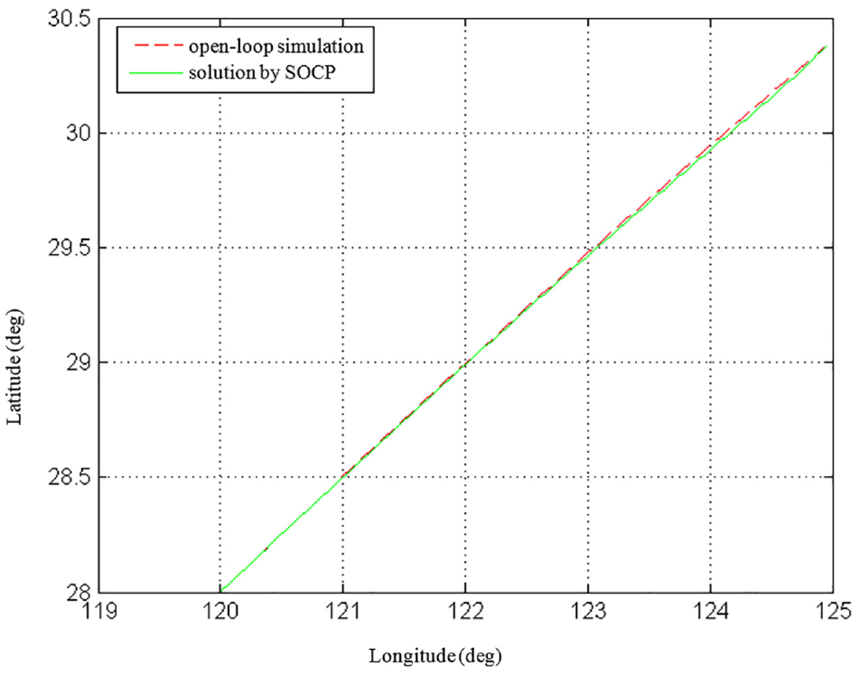
Ground track comparison.

Figure 6.

Altitude comparison.

Figure 7.

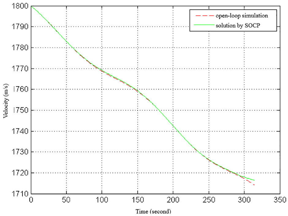
Velocity comparison.

Single uncertain NFZ

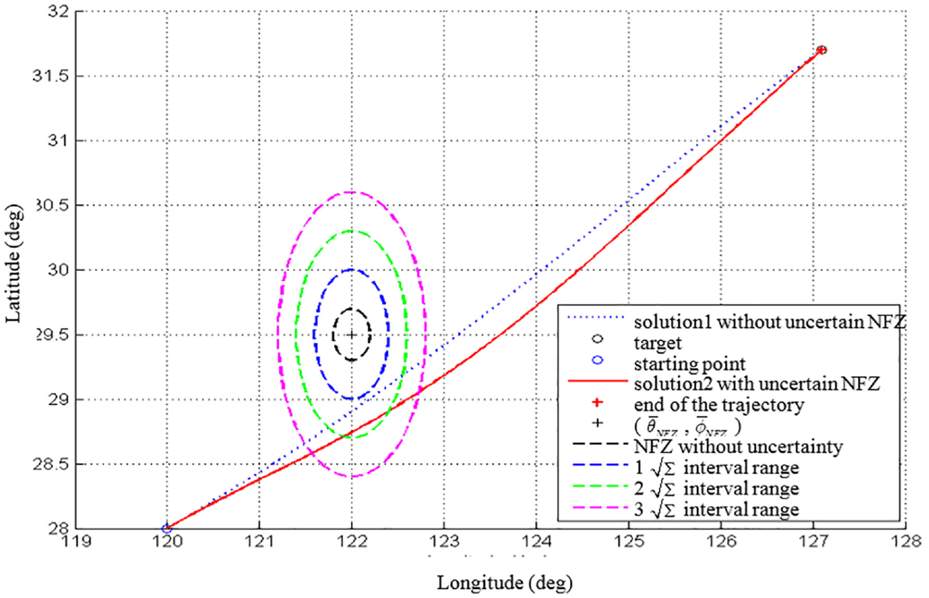
In this mission, we assume that there is an uncertain cylindrical NFZ_R, the center coordinates of which are difficult to determine. The source of uncertainty can be vague intelligence, modeling errors, or movement of the NFZ_R itself. However, an initial guess of the center coordinates $({\overline{\theta }}_{\mathrm{NFZ}},{\overline{\varphi }}_{\mathrm{NFZ}})$ can be given. Without loss of generality, NFZ_R’s real center coordinates satisfy individual Gaussian distribution. By measuring the speed and heading of the object, the standard deviation $({\Sigma }_{\theta }^{1/2},{\Sigma }_{\varphi }^{1/2})$ of its position after a period of time can also be estimated. Unfortunately, the area where NFZ_R may exist (NFZ_P) just blocks the way to target, and bypassing the NFZ_P exceeds the vehicle’s capacity. So it is inevitable to bear the risk and fly through the NFZ_P. The probability of success threshold P* is set to 90%, which means that the probability of the vehicle not flying through the NFZ_R and reaching the target should be greater than or equal to 90%. The performance index is

$$\mathrm{minimize}\mathit{J}={\mathit{J}}_1+{\kappa }_3{\mathit{J}}_3$$

(99)

which helps ABHV reach the target in the shortest time.

The initial and terminal conditions of the mission are given in Table 4. The target has a downrange of 792.2 km and a left crossrange of 107.6 km. The values of the limits in the path constraints are as follows: ${\stackrel{·}{Q}}_{\max }=500\mathrm{kW}/{\mathrm{m}}^2$ , $q_{\max }=80000N/m^2$ , and $n_{\max }=2.0g_0$ . In addition, the upper bounds on the magnitude of the bank angle are set at ${\sigma }_{\max }=60\mathrm{deg}$ . The parameters of uncertain NFZ are given in Table 5.

Table 4.

Initial and terminal conditions.

States	r, km	V, m/s	$\gamma$ , deg	$\theta$ , deg	$\varphi$ , deg	$\psi$ , deg	m, kg
x 0	27.0	1800.0	0.0	120.0	28.0	60.0	2944
x f	27	-	-	127.1	31.7	-	2221

Table 5.

Parameters of uncertain NFZ.

Parameters	P*	${\overline{\theta }}_{\mathrm{NFZ}}$ , deg	${\overline{\varphi }}_{\mathrm{NFZ}}$ , deg	$\sqrt{{\Sigma }_{\theta \_\mathrm{NFZ}}}$ , deg	$\sqrt{{\Sigma }_{\varphi \_\mathrm{NFZ}}}$ , deg	$d_{\mathrm{NFZ}}$ , km
Value	90%	122.0	29.5	0.2	0.3	22

Figure 8 shows the ground track. For comparison, the solution without uncertain NFZ is also obtained as the baseline. Both trajectories do fly through the NFZ_P, but the solution that considering the uncertain NFZ is farther away from the $({\overline{\theta }}_{\mathrm{NFZ}},{\overline{\varphi }}_{\mathrm{NFZ}})$ compares with the baseline one. To verify the correctness of the trajectory, the 68–95–99.7 rule is introduced. The baseline trajectory is quite close to the $1\sqrt{\Sigma }$ boundary, which means the probability of success is only about 68%. Thus, it does not meet the mission requirements. Solution 2 steers away from the NFZ center, grazes $2\sqrt{\Sigma }$ the boundary, which means that the probability of success is slightly less than 95%, larger than the threshold P*. This figure illustrates the proposed algorithm can successfully handle the uncertain NFZ problem.

Figure 8.

Ground track comparison.

More comparison is given in Figures 9 to 13. In Figure 9 we can see the vehicle turns right then left to steer away from the uncertain NFZ in solution 2. Its trajectory is more curved than the baseline. Figure 12 shows that angle of attack and throttle changes with flight conditions. As the altitude decreases, the air density gradually increases, so the required trim angle of attack decreases. This will result in a decrease in drag and the throttle required. The heating rate and dynamic pressure, and normal load histories are plotted in Figure 13. All two solution satisfies path constraints.

Figure 9.

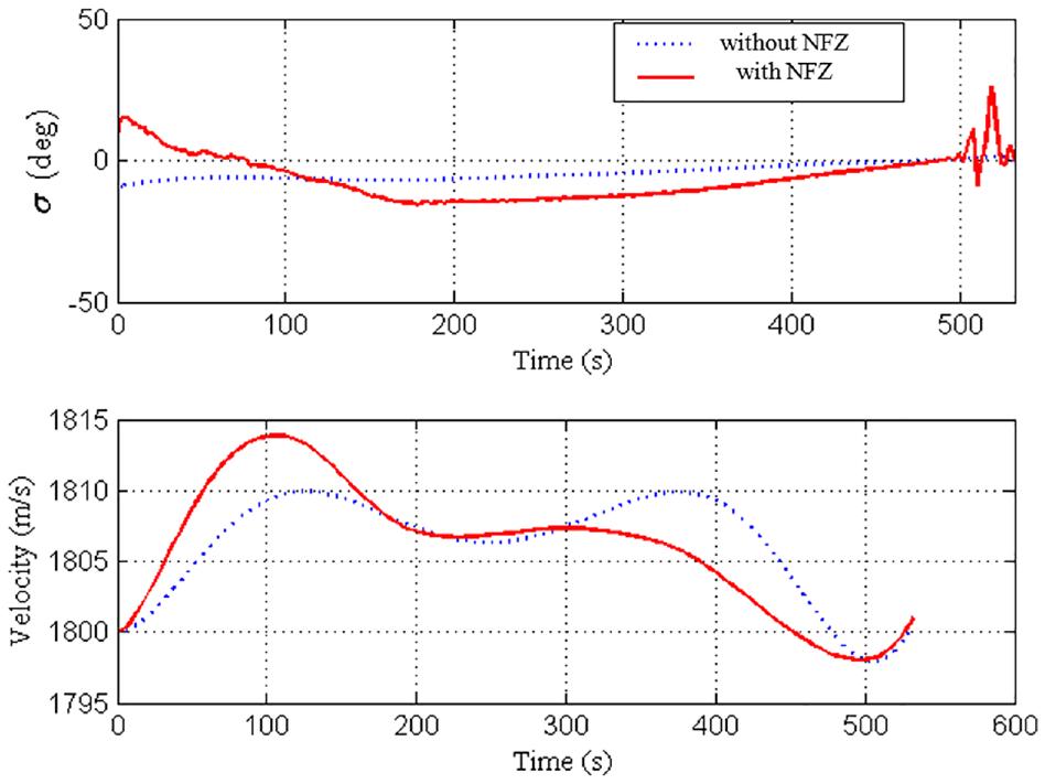
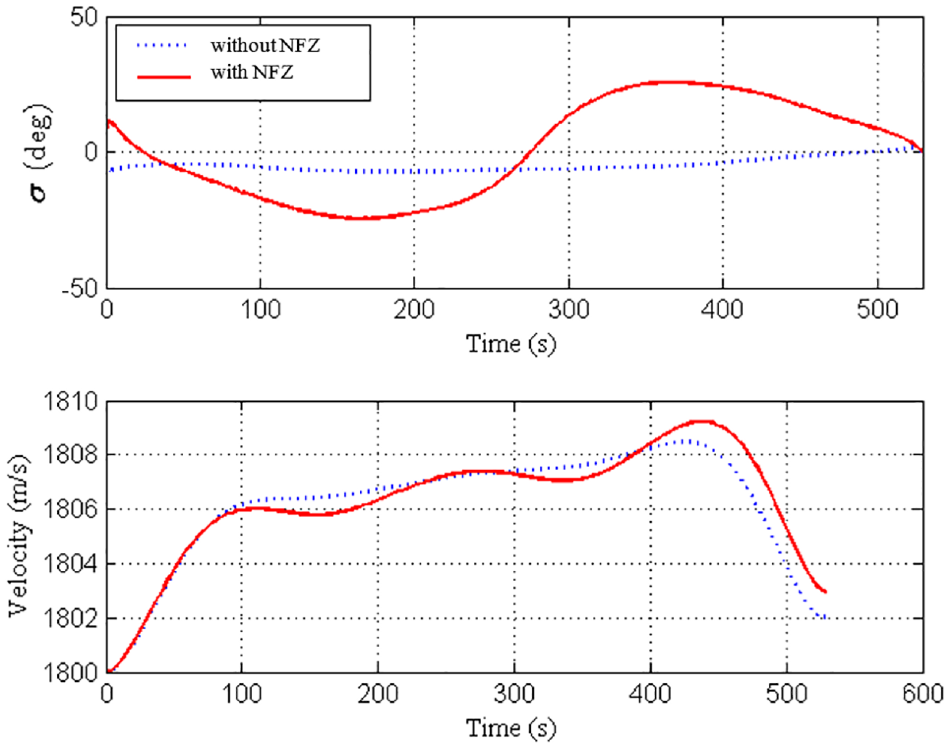
Bank angle and velocity comparison.

Figure 10.

Altitude and heading comparison.

Figure 11.

Flight-path angle comparison.

Figure 12.

Angle of attack and throttle comparison.

Figure 13.

Heating rate, dynamic pressure, and normal load histories.

Multiple uncertain NFZs

In this mission, we assume that there exist two uncertain NFZs (Table 6). The areas where they may exist happens to be on the path to the target. The vehicle’s path constraints, initial and terminal conditions are the same as in section 4.3. Use the method described in section 4.2 to handle multiple chance constraints. The value of the probability of success threshold P* is still 90%.

Table 6.

Parameters of uncertain NFZs.

Parameters	${\overline{\theta }}_{\mathrm{NFZ}}$ , deg	${\overline{\varphi }}_{\mathrm{NFZ}}$ , deg	${\Sigma }_{\theta }^{1/2}$ , deg	${\Sigma }_{\varphi }^{1/2}$ , deg	$d_{\mathrm{NFZ}}$ , km
NFZ1	122.0	29.6	0.2	0.3	22
NFZ2	125.0	30.1	0.2	0.1	22

The ground track of the solution subject to the multiple NFZs chance constraints is shown in Figure 14.

Figure 14.

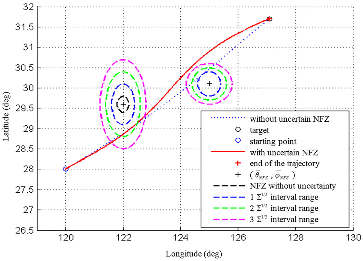
Ground track with two uncertain NFZs.

The trajectory without NFZ constraints flies through both NFZ_P, whereas the trajectory with the uncertain NFZ constraints grazes the 90% boundary. In order to verify the correctness of the results, a Monte Carlo simulation was carried out. First, 1000 NFZs combinations that follow the distribution in Table 6 are randomly generated. Next, we check whether the trajectory violates the constraints formed by the these NFZs combinations. Table 7 shows that the trajectory has a 91.7% probability of not colliding with the real no-fly zone, which is higher than the set threshold. This result strongly supports the method in this paper.

Table 7.

Monte Carlo simulation.

	Collision	No-collision	Total	Success rate
Value	83	917	1000	91.7%

The corresponding control input and states are shown in Figures 15 and 16.

Figure 15.

Bank angle and velocity comparison.

Figure 16.

Altitude and heading comparison.

Capability test

The previous section demonstrates that the algorithm can handle multiple uncertain no-fly zones. Then, further tests were performed to show how the shape and location of uncertain NFZs influenced the trajectory, in other words, how robust the new algorithm is.

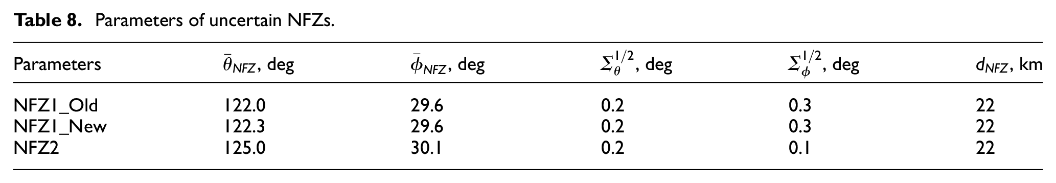
The position of NFZ1 is changed to compress the vehicle’s activity space (Table 8). We want to test whether the vehicle can still satisfy the chance constraint under more extreme conditions.

Table 8.

Parameters of uncertain NFZs.

Parameters	${\overline{\theta }}_{\mathrm{NFZ}}$ , deg	${\overline{\varphi }}_{\mathrm{NFZ}}$ , deg	${\Sigma }_{\theta }^{1/2}$ , deg	${\Sigma }_{\varphi }^{1/2}$ , deg	$d_{\mathrm{NFZ}}$ , km
NFZ1_Old	122.0	29.6	0.2	0.3	22
NFZ1_New	122.3	29.6	0.2	0.3	22
NFZ2	125.0	30.1	0.2	0.1	22

Compared to the previous simulation results, the vehicle performs a more violent maneuver when approaching NFZ1 to achieve a given success rate (Figure 17). Similarly, a Monte Carlo simulation is performed for the new trajectory (Table 9), which guarantees the satisfaction of chance constraints (92.3% > p*).

Figure 17.

Ground track with the distance between two uncertain NFZs changed.

Table 9.

Monte Carlo simulation.

	Collision	No-collision	Total	Success rate
Value	77	923	1000	92.3%

In addition, we change the variance of the coordinate position of the NFZ’s center (Table 10). Table 11 and Figure 18 demonstrate the same conclusion: the algorithm proposed in this paper has a strong robustness.

Table 10.

Parameters of uncertain NFZs.

Parameters	${\overline{\theta }}_{\mathrm{NFZ}}$ , deg	${\overline{\varphi }}_{\mathrm{NFZ}}$ , deg	${\Sigma }_{\theta }^{1/2}$ , deg	${\Sigma }_{\varphi }^{1/2}$ , deg	$d_{\mathrm{NFZ}}$ , km
NFZ1_Old	122.0	29.6	0.2	0.3	22
NFZ1_New	122.0	29.6	0.3	0.4	22
NFZ2	125.0	30.1	0.2	0.1	22

Table 11.

Monte Carlo simulation.

	Collision	No-collision	Total	Success rate
Value	95	905	1000	90.5%

Figure 18.

Ground track with the variance of uncertain NFZs changed.

Conclusion

According to the flight characteristics of ABHV, this paper proposes a hybrid optimization method first. The numerical demonstrations show that this method can effectively solve the trajectory optimization problem of ABHV. Then we discuss the situation with uncertain NFZ. As a result, the uncertain NFZs that may exist are modeled as chance constraints. On this basis, a convexification method is proposed, which can convert the concave chance constraint into a deterministic constraint that can be solved by convex optimization. Furthermore, it is further extended to situations where there are multiple uncertain NFZs.

In the past research, environmental uncertainty in hypersonic vehicle trajectory optimization was rarely discussed, let alone integrated into the optimization algorithm. The preliminary results obtained expand our understanding of convex optimization in complex aerospace engineering.