Influence of transport coefficients’ dependence on temperature for gas flow in microbearing

Abstract

The paper presents an analytical solution for the non-isothermal compressible gas flow in a slide microbearing with different temperatures of walls. The gas flow is defined by the Navier-Stokes-Fourier system of the continuum equations and first order boundary conditions. Knudsen number corresponds to the slip and continuum flow (Kn ≤ 10⁻¹) and Reynolds number is moderately high, so inertia needs to be included. The solution is obtained by perturbations with the first approximation that relates to the continuum flow and the second one that involves second-order effects: the rarefaction, inertia, convection, dissipation, and rate at which work is done in compressing the element of fluid. The presented model analyzes the influence of the dependence of transport coefficients on temperature. The obtained analytical solution for the pressure, velocity, and temperature is approved by a comparison with the results of other authors. The microbearings can often be a part of MEMS, so the presented method and the obtained analytical solution can serve for solving similar non-isothermal shear-driven or pressure-driven problems. The paper gives an estimation about the error in values for microbearing mass flow and load capacity if the dependence of transport coefficients on temperature are neglected.

Introduction

Micro-Electro-Mechanical-Systems (MEMS) very often contain micro-channels with a pressure-driven or shear-driven gas flow.^1,2 In some of them, the gas flow can serve as a lubricant that reduces the sliding friction between solid walls. The walls can be parallel, like those in micro-combs, or inclined, like those in microbearings. The walls can also be on similar or, more frequently, on different temperatures. These walls can be, for example, the magnetic disk and the head slider in hard disk drives. A high recording density can be accomplished by heat-assisted magnetic recording, where the magnetic disk is locally heated using a laser beam. Also, a microbearing could be part of a microengine with a wall in contact with the combustion chamber. In these and similar cases, there is a significant temperature difference between the walls that affects the lubrication, so the lubrication analysis could not assume isothermal flow and the thermal effects on the microbearing performance should be evaluated. Besides, the transport coefficients dependence on temperature should be considered. Because of that, the results in this field have wide application and significant practical importance; hence, many researchers deal with gas flow in this domain.

Traditionally, the continuum gas flow in bearings is modeled by the Reynolds lubrication equation. It is derived from the Navier-Stokes and continuity equations under the no-slip boundary conditions (Kn = 0). In microbearings, the thickness of the lubricating film is of the order of the mean free path of gas molecules and the continuum theory fails. Knudsen number is not negligible anymore. Among a wide range of Knudsen numbers in micro-flows, the slip flow (10⁻³ < Kn < 10⁻¹) is encountered more often. Therefore, the solutions for the slip gas flow in microbearings are desirable.

The slip gas flow in microbearings has been analyzed mostly numerically, using two main directions. The first one is by solving the Reynolds equation obtained from a model of the linearized Boltzmann equation, frequently from the Bhatnagar–Gross–Krook^3,5–10 (BGK) model. The second one uses the Direct Simulation Monte Carlo (DSMC) method^11–13.

Many authors have used different boundary conditions to correct the Reynolds lubrication equation and enhance its solution to the rarefied domain. Burgdorfer ³ was the first who included the Maxwell’s first-order slip boundary condition ⁴ to expand the Reynolds equation scope to the slip domain. Several authors corrected the order of the condition at the wall: Mitsuya ⁵ to the 1.5-order slip model for ultra-thin gas lubrication, and Hsia and Domoto ⁶ using their second-order boundary condition in the Reynolds lubrication equation. They compared the obtained results with the results of experiments with different gases in microbearings.

A more sophisticated slip correction of the Reynolds equation was obtained by Fukui and Kaneko, ⁷ who enabled the solutions for arbitrary Knudsen numbers. They introduced the flow rate coefficient Q_p of the Poiseuille flow to the lubrication equation. Furthermore, Fukui and Kaneko ⁸ gave a database of tabulated values of the flow rate coefficient for different Knudsen numbers and explicit power series expressions Q_p(Kn) with an error less than 1%. Sun et al. ⁹ modified the Reynolds equation using the corrected dynamic viscosity. Bahukudumbi and Beskok ¹⁰ introduced the generalized dynamic viscosity to obtain a new modified Reynolds equation that enabled the solution for the entire range of Knudsen numbers. Gu et al. ¹¹ derived an extended Reynolds equation based on the regularized 13 moment equations and lubrication theory for gas slider bearings operating in the transition regime.

Many researchers used DSMC. Alexander et al. ¹² and Liu and Ng ¹³ approved their DSMC results by a comparison with numerical results obtained with the BGK model of kinetic equation. They gave a wide spectrum of results for different bearing numbers and different inclination angles. Myo et al. ¹⁴ applied DSMC for both pure gas and gas mixtures.

All these solutions have been obtained for the isothermal flow condition; there are few results for the non-isothermal flow conditions in microbearings. Based on the Bhatnagar–Gross–Krook–Welander (BGKW) model of the Boltzmann equation, Doi ¹⁵ studied micro-lubrication between nearly parallel walls with both equal and different temperatures. Our model presented in this paper is in good agreement with Doi ¹⁵ results.

The perturbation model, used in this paper, was verified in our previous work^16–19 for: isothermal microbearing gas flow, ¹⁶ non-isothermal gas flow with equal temperatures of the walls,^17,18 and non-isothermal microbearing gas flow with different temperatures of the walls obtained for constant viscosity and thermal conductivity. ¹⁹

In this paper, a non-isothermal microbearing slip gas flow is analyzed by including the dependence of transport coefficients on the temperature. The solution for pressure, velocity, and temperature fields is obtained for moderately high Reynolds numbers by perturbations. Two approximations are defined. The first corresponds to the continuum, and the second one to the rarefied gas flow. Since the flow condition is with moderately high Reynolds numbers, the second approximation includes also: inertia, convection, dissipation, and rate at which work is done in compressing the element of fluid. It is shown that there is a deviation between the load capacity, as well as the microbearing mass flow rate, in relation with the values of the load capacity and the mass flow rate obtained by neglecting the dependence of transport coefficients on the temperature. The paper gives an estimation of the error for the load capacity and the mass flow when the dynamic viscosity and thermal conductivity dependence on the temperature are neglected.

Problem description and solution

A steady compressible rarefied two-dimensional non-isothermal subsonic shear-driven gas flow in a microbearing with different temperature of the walls for slip and continuum regimes has been analyzed by the macroscopic approach (Figure 1).

Figure 1.

Slider microbearing geometry.

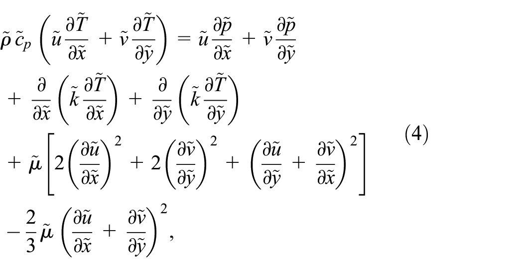
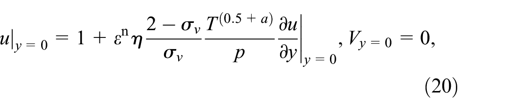
The slip gas flow calls for the boundary conditions for the velocity and temperature at the walls that differ from the boundary conditions for the continuum regime where Kn→0. In accordance with the slip flow theory,^1,2 these boundary conditions manifest as: the difference between the velocity of gas at the wall and the velocity of the wall (velocity slip), and the difference between the temperature of the gas at the wall and the temperature of the wall (temperature jump). For such a gas flow in microbearings, the continuity, the Navier-Stokes equations for streamwise direction $\tilde{x}$ and crosswise direction $\tilde{y}$ , the energy equation and the equation of state, as well as the slip velocity and temperature jump Maxwell-Smoluchowski first-order boundary conditions ⁴ at the walls are:

$$\frac{\partial \left(\tilde{\rho }\tilde{u}\right)}{\partial \tilde{x}}+\frac{\partial \left(\tilde{\rho }\tilde{v}\right)}{\partial \tilde{y}}=0,$$

(1)

$$\begin{array}{c}\tilde{\rho }(\tilde{u}\frac{\partial \tilde{u}}{\partial \tilde{x}}+\tilde{v}\frac{\partial \tilde{u}}{\partial \tilde{y}})=-\frac{\partial \tilde{p}}{\partial \tilde{x}}\hfill \\ +\frac{\partial }{\partial \tilde{x}}[2\tilde{\mu }\frac{\partial \tilde{u}}{\partial \tilde{x}}-\frac{2}{3}\tilde{\mu }(\frac{\partial \tilde{u}}{\partial \tilde{x}}+\frac{\partial \tilde{v}}{\partial \tilde{y}})]+\frac{\partial }{\partial \tilde{y}}\left[\tilde{\mu }(\frac{\partial \tilde{u}}{\partial \tilde{y}}+\frac{\partial \tilde{v}}{\partial \tilde{x}})\right],\hfill \end{array}$$

(2)

$$\begin{array}{c}\tilde{\rho }(\tilde{u}\frac{\partial \tilde{v}}{\partial \tilde{x}}+\tilde{v}\frac{\partial \tilde{v}}{\partial \tilde{y}})=-\frac{\partial \tilde{p}}{\partial \tilde{y}}\hfill \\ +\frac{\partial }{\partial \tilde{y}}[2\tilde{\mu }\frac{\partial \tilde{v}}{\partial \tilde{y}}-\frac{2}{3}\tilde{\mu }(\frac{\partial \tilde{u}}{\partial \tilde{x}}+\frac{\partial \tilde{v}}{\partial \tilde{y}})]+\frac{\partial }{\partial \tilde{x}}\left[\tilde{\mu }(\frac{\partial \tilde{u}}{\partial \tilde{y}}+\frac{\partial \tilde{v}}{\partial \tilde{x}})\right],\hfill \end{array}$$

(3)

$$\begin{array}{c}\tilde{\rho }{\tilde{c}}_p(\tilde{u}\frac{\partial \tilde{T}}{\partial \tilde{x}}+\tilde{v}\frac{\partial \tilde{T}}{\partial \tilde{y}})=\tilde{u}\frac{\partial \tilde{p}}{\partial \tilde{x}}+\tilde{v}\frac{\partial \tilde{p}}{\partial \tilde{y}}\hfill \\ +\frac{\partial }{\partial \tilde{x}}\left(\tilde{k}\frac{\partial \tilde{T}}{\partial \tilde{x}}\right)+\frac{\partial }{\partial \tilde{y}}\left(\tilde{k}\frac{\partial \tilde{T}}{\partial \tilde{y}}\right)\hfill \\ +\tilde{\mu }[2{\left(\frac{\partial \tilde{u}}{\partial \tilde{x}}\right)}^2+2{\left(\frac{\partial \tilde{v}}{\partial \tilde{y}}\right)}^2+{(\frac{\partial \tilde{u}}{\partial \tilde{y}}+\frac{\partial \tilde{v}}{\partial \tilde{x}})}^2]\hfill \\ -\frac{2}{3}\tilde{\mu }{(\frac{\partial \tilde{u}}{\partial \tilde{x}}+\frac{\partial \tilde{v}}{\partial \tilde{y}})}^2,\hfill \end{array}$$

(4)

$$\frac{\tilde{p}}{\tilde{\rho }}=\tilde{R}\tilde{T},$$

(5)

$$\begin{array}{c}{\tilde{u}|}_{\tilde{y}=0}={\tilde{u}}_{\mathrm{w}}+\frac{2-{\sigma }_v}{{\sigma }_v}\tilde{\lambda }{\frac{\partial \tilde{u}}{\partial \tilde{y}}|}_{\tilde{y}=0},{\tilde{V}|}_{\tilde{y}=0}=0,\hfill \\ {\tilde{u}|}_{\tilde{y}=\tilde{h}}=-\frac{2-{\sigma }_v}{{\sigma }_v}\tilde{\lambda }{\frac{\partial \tilde{u}}{\partial \tilde{y}}|}_{\tilde{y}=\tilde{h}},{\tilde{V}|}_{\tilde{y}=\tilde{h}}=\tilde{u}{\frac{\mathrm{d}\tilde{h}}{\mathrm{d}\tilde{x}}|}_{\tilde{y}=\tilde{h}},\hfill \end{array}$$

(6)

$$\begin{array}{c}{\tilde{T}|}_{\tilde{y}=0}={\tilde{T}}_{\mathrm{w}1}+\frac{2-{\sigma }_T}{{\sigma }_T}\left(\frac{2\kappa }{\kappa +1}\right)\frac{\tilde{\lambda }}{\mathrm{Pr}}{\frac{\partial \tilde{T}}{\partial \tilde{y}}|}_{\tilde{y}=0},\hfill \\ {\tilde{T}|}_{\tilde{y}=\tilde{h}}={\tilde{T}}_{\mathrm{w}2}-\frac{2-{\sigma }_T}{{\sigma }_T}\left(\frac{2\kappa }{\kappa +1}\right)\frac{\tilde{\lambda }}{\mathrm{Pr}}{\frac{\partial \tilde{T}}{\partial \tilde{y}}|}_{\tilde{y}=\tilde{h}},\hfill \end{array}$$

(7)

where σ _v and σ _T are the momentum and energy accommodation coefficients respectively, κ is the ratio of specific heats, $\mathrm{Pr}={\tilde{c}}_p\tilde{\mu }/\tilde{k}$ is the Prandtl number, and ${\tilde{c}}_p$ is the specific heat at the constant pressure. This system of equations (1)–(7) has been transformed into the non-dimensional form by the next scales: the exit microbearing height ${\tilde{h}}_{\mathrm{e}}$ for crosswise coordinate $\tilde{y}$ and microbearing height $\tilde{h}$ , the microbearing length $\tilde{l}$ for streamwise coordinate $\tilde{x}$ , the wall velocity ${\tilde{u}}_{\mathrm{w}}$ for the velocity components $\tilde{u}$ and $\tilde{v}$ , the average temperature of the lower ${\tilde{T}}_{\mathrm{w}1}$ and the upper ${\tilde{T}}_{\mathrm{w}2}$ wall ${\tilde{T}}_{\mathrm{r}}=({\tilde{T}}_{\mathrm{w}1}+{\tilde{T}}_{\mathrm{w}2})/2$ for the temperature $\tilde{T}$ . Pressure $\tilde{p}$ has been scaled by the pressure at the microbearing exit cross section ${\tilde{p}}_{\mathrm{e}}$ (inlet pressure ${\tilde{p}}_{\mathrm{i}}$ is the same as exit pressure ${\tilde{p}}_{\mathrm{e}}$ , ${\tilde{p}}_{\mathrm{i}}={\tilde{p}}_{\mathrm{e}}$ ) and density $\tilde{\rho }$ by ${\tilde{\rho }}_{\mathrm{e}}={\tilde{p}}_{\mathrm{e}}/\tilde{R}{\tilde{T}}_{\mathrm{r}}$ , where $\tilde{R}$ is the gas constant. Dynamic viscosity $\tilde{\mu }$ and thermal conductivity $\tilde{k}$ have been scaled by their reference values ${\tilde{\mu }}_{\mathrm{r}}$ and ${\tilde{k}}_{\mathrm{r}}$ , which both correspond to the reference temperature ${\tilde{T}}_{\mathrm{r}}$ . The molecular mean-free path $\tilde{\lambda }=\tilde{\mu }\sqrt{\pi \tilde{R}\tilde{T}/2}/\tilde{p}$ has been scaled by the reference molecular mean-free path ${\tilde{\lambda }}_{\mathrm{r}}={\tilde{\mu }}_{\mathrm{r}}\sqrt{\pi \tilde{R}{\tilde{T}}_{\mathrm{r}}/2}/{\tilde{p}}_{\mathrm{e}}$ . All the dimensional variables are signed with a tilde (∼), while the dimensionless are without it: $x=\tilde{x}/\tilde{l},y=\tilde{y}/{\tilde{h}}_{\mathrm{e}},$ $h=\tilde{h}/{\tilde{h}}_{\mathrm{e}},u=\tilde{u}/{\tilde{u}}_{\mathrm{w}},$ $v=\tilde{v}/{\tilde{u}}_{\mathrm{w}},T=\tilde{T}/{\tilde{T}}_{\mathrm{r}},$ $p=\tilde{p}/{\tilde{p}}_{\mathrm{e}},\rho =\tilde{\rho }/{\tilde{\rho }}_{\mathrm{e}},$ $\mu =\tilde{\mu }/{\tilde{\mu }}_{\mathrm{r}},k=\tilde{k}/{\tilde{k}}_{\mathrm{r}},$ and $\lambda =\tilde{\lambda }/{\tilde{\lambda }}_{\mathrm{r}}$ . The dimensionless microbearing height h(x) has been defined as h(x)=h_i-x(h_i-1), where h_i is the dimensionless inlet microbearing height.

To estimate the order of each term in the system of dimensionless governing equations and boundary conditions, we have defined a small parameter ε as the ratio between the exit microbearing height and the microbearing length:

$$\epsilon ={\tilde{h}}_{\mathrm{e}}/\tilde{l},(\epsilon <<1).$$

(8)

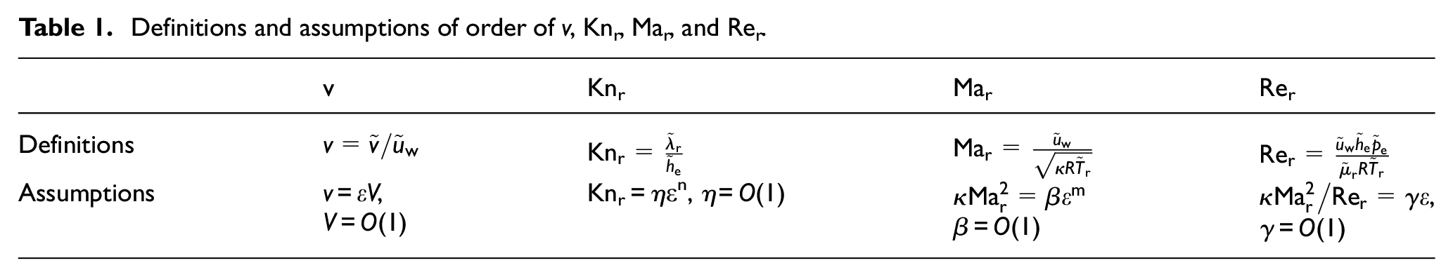
Moreover, we have proposed the next four assumptions to define the order of the dimensionless crosswise velocity component v, reference Knudsen, Reynolds, and Mach numbers, correlating them with the small parameter ε. All the other dimensionless variables are supposed to be of order O(1).

• 1. The slope of the upper microbearing wall is assumed to be small, which implies that the crosswise velocity component $\tilde{v}$ is much smaller than the streamwise component $\tilde{u}$ . Then, v is of the order O(ε), so we can write:

$$v=\epsilon V,\mathrm{where}V=O\left(1\right).$$

(9)

• 2. The presumption of the slip gas flow means that Knudsen number is small, so it is possible to assume:

$$\mathrm{K}{\mathrm{n}}_{\mathrm{r}}=\eta {\epsilon }^{\mathrm{n}},\mathrm{where}\mathrm{n}>0\mathrm{and}\eta =O\left(1\right),$$

(10)

where $\mathrm{K}{\mathrm{n}}_{\mathrm{r}}$ is the reference Knudsen number defined as $\mathrm{K}{\mathrm{n}}_{\mathrm{r}}={\tilde{\lambda }}_{\mathrm{r}}/{\tilde{h}}_{\mathrm{e}}$ .

• 3. Since the flow is subsonic, the Mach number is also small, so we can assume:

$$\kappa {\mathrm{Ma}}_{\mathrm{r}}^2=\beta {\epsilon }^{\mathrm{m}},\mathrm{where}\mathrm{m}>0\mathrm{and}\mathrm{\beta }=\mathrm{O}\left(1\right),$$

(11)

where Ma_r is the reference Mach number defined as $\mathrm{M}{\mathrm{a}}_{\mathrm{r}}={\tilde{u}}_{\mathrm{w}}/\sqrt{\kappa R{\tilde{T}}_{\mathrm{r}}}$ .

• 4. It is assumed also that the ratio between the square of the Mach number and Reynolds number is also of the order of the small parameter:

$$\frac{\kappa {\mathrm{Ma}}_{\mathrm{r}}^2}{\mathrm{R}{\mathrm{e}}_{\mathrm{r}}}=\gamma \epsilon ,\mathrm{where}\gamma =O\left(1\right),$$

(12)

where Re_r is the reference Reynolds number defined as ${\mathrm{Re}}_{\mathrm{r}}={\tilde{u}}_{\mathrm{w}}{\tilde{h}}_{\mathrm{e}}{\tilde{p}}_{\mathrm{e}}/{\tilde{\mu }}_{\mathrm{r}}R{\tilde{T}}_{\mathrm{r}}$ .

The parameters V, η, β, γ, n, and m in the previous assumptions ensure the flexibility to the model. Namely, involving those parameters enable applying the model to different flow conditions (different values of Kn_r, Ma_r, and Re_r) for one defined geometry of microbearing, that is, ε. Besides, V, η, β, γ have to be O(1), to enable that v∼ε, Kn_r∼εⁿ, $\kappa {\mathrm{Ma}}_{\mathrm{r}}^2~{\epsilon }^{\mathrm{m}}$ , and $\kappa {\mathrm{Ma}}_{\mathrm{r}}^2/\mathrm{R}{\mathrm{e}}_{\mathrm{r}}~\epsilon$ .

In Table 1, we summarize the definitions and assumptions about the order of crosswise velocity v, the reference Knudsen, Mach, Reynolds numbers, and parameters V, η, β, and γ.

Table 1.

Definitions and assumptions of order of v, Kn_r, Ma_r, and Re_r.

	v	Knr	Mar	Rer
Definitions	$v=\tilde{v}/{\tilde{u}}_{\mathrm{w}}$	$\mathrm{K}{\mathrm{n}}_{\mathrm{r}}=\frac{{\tilde{\lambda }}_{\mathrm{r}}}{{\tilde{h}}_{\mathrm{e}}}$	$\mathrm{M}{\mathrm{a}}_{\mathrm{r}}=\frac{{\tilde{u}}_{\mathrm{w}}}{\sqrt{\kappa R{\tilde{T}}_{\mathrm{r}}}}$	${\mathrm{Re}}_{\mathrm{r}}=\frac{{\tilde{u}}_{\mathrm{w}}{\tilde{h}}_{\mathrm{e}}{\tilde{p}}_{\mathrm{e}}}{{\tilde{\mu }}_{\mathrm{r}}R{\tilde{T}}_{\mathrm{r}}}$
Assumptions	v = εV, V = O(1)	Knr = ηεn, η = O(1)	$\kappa {\mathrm{Ma}}_{\mathrm{r}}^2=\beta {\epsilon }^{\mathrm{m}}$ β = O(1)	$\kappa {\mathrm{Ma}}_{\mathrm{r}}^2/\mathrm{R}{\mathrm{e}}_{\mathrm{r}}=\gamma \epsilon$ , γ = O(1)

Regardless of the different possibilities for modeling both the viscosity and thermal conductivity dependence on temperature, ²⁰ the hard sphere molecular model has been used here to express the dynamic viscosity μ and heat conductivity k in terms of temperature using the power law ²¹ :

$$\begin{array}{c}\tilde{\mu }/{\tilde{\mu }}_{\mathrm{r}}={\tilde{T}}^a/{\tilde{T}}_{\mathrm{r}}^a\mathrm{i}.\mathrm{e}.\mu =T^a,\mathrm{and}\hfill \\ \tilde{k}/{\tilde{k}}_{\mathrm{r}}={\tilde{T}}^a/{\tilde{T}}_{\mathrm{r}}^a\mathrm{i}.\mathrm{e}.k=T^a,\hfill \end{array}$$

(13)

where a is the viscosity-temperature index which ranges from a = 0.5, for the elastic sphere molecule model, to a = 1, for the Maxwellian molecules. ²¹ The relation between the local $\mathrm{Kn}=\tilde{\lambda }/{\tilde{h}}_{\mathrm{e}}$ and the reference Knudsen number Kn_r then follows:

$$\mathrm{Kn}=\lambda \mathrm{K}{\mathrm{n}}_{\mathrm{r}}=\frac{T{}^{(a+0.5)}}{p}\mathrm{K}{\mathrm{n}}_{\mathrm{r}},$$

(14)

Now, the system of governing equations and boundary conditions (1)−(7) in the dimensionless form follow:

$$\frac{\partial \left(\rho u\right)}{\partial x}+\frac{\partial \left(\rho V\right)}{\partial y}=0,$$

(15)

$${\epsilon }^{\mathrm{m}}\beta \rho (u\frac{\partial u}{\partial x}+V\frac{\partial u}{\partial y})=-\frac{\partial p}{\partial x}+\gamma \frac{\partial }{\partial y}\left(\mu \frac{\partial u}{\partial y}\right)+O({\epsilon }^2),$$

(16)

$$\frac{\partial p}{\partial y}=O({\epsilon }^2),$$

(17)

$$\begin{array}{c}{\epsilon }^{\mathrm{m}}\frac{\beta }{\gamma }\mathrm{Pr}\rho (u\frac{\partial T}{\partial x}+V\frac{\partial T}{\partial y})=\frac{\partial }{\partial y}\left(k\frac{\partial T}{\partial y}\right)\hfill \\ +{\epsilon }^{\mathrm{m}}\frac{\kappa -1}{\kappa }\beta \mathrm{Pr}[\frac{1}{\gamma }u\frac{\partial p}{\partial x}+\mu {\left(\frac{\partial u}{\partial y}\right)}^2]+O({\epsilon }^2),\hfill \end{array}$$

(18)

$$p=\rho T.$$

(19)

$${u|}_{y=0}=1+{\epsilon }^{\mathrm{n}}\eta \frac{2-{\sigma }_v}{{\sigma }_v}\frac{T^{(0.5+a)}}{p}{\frac{\partial u}{\partial y}|}_{y=0},V_{y=0}=0,$$

(20)

$$\begin{array}{c}{u|}_{y=h\left(x\right)}=-{\epsilon }^{\mathrm{n}}\eta \frac{2-{\sigma }_v}{{\sigma }_v}{\frac{T^{(0.5+a)}}{p}\frac{\partial u}{\partial y}|}_{y=h\left(x\right)},\hfill \\ V_{y=h\left(x\right)}=u\frac{\mathrm{d}h\left(x\right)}{\mathrm{d}x},\hfill \end{array}$$

(21)

$${T|}_{y=0}=1+\theta +{\epsilon }^{\mathrm{n}}\eta \frac{2-{\sigma }_T}{{\sigma }_T}\left(\frac{2\kappa }{\kappa +1}\right)\frac{1}{\mathrm{Pr}}\frac{T^{(0.5+a)}}{p}{\frac{\partial T}{\partial y}|}_{y=0},$$

(22)

$$\begin{array}{c}\multicolumn{1}{c}{{T|}_{y=h\left(x\right)}=1-\theta -{\epsilon }^{\mathrm{n}}\eta \frac{2-{\sigma }_T}{{\sigma }_T}\left(\frac{2\kappa }{\kappa +1}\right)}\\ \frac{1}{\mathrm{Pr}}\frac{T^{(0.5+a)}}{p}{\frac{\partial T}{\partial y}|}_{y=h\left(x\right)},\hfill \end{array}$$

(23)

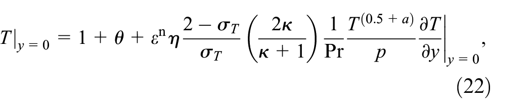
where θ = (T_w1–T_w2)/2.

There is another dimensionless quantity which appears in the analysis of gas flows in microbearings. It is the bearing number Λ defined as:

$$\mathrm{\Lambda }=\frac{6{\tilde{\mu }}_{\mathrm{r}}{\tilde{u}}_{\mathrm{w}}\tilde{l}}{{\tilde{p}}_{\mathrm{e}}{\tilde{h}}_{\mathrm{e}}^2}.$$

(24)

Our coefficient γ, which occurs naturally in the dimensionless momentum equation (16) and energy equation (18), represents the bearing number Λ, as from equations (12) and (24) it follows that γ = Λ/6. Besides, the bearing number Λ can be expressed in terms of the reference Mach number, Reynolds number, and the small parameter ε as $\mathrm{\Lambda }=\frac{6\kappa {\mathrm{Ma}}_{\mathrm{r}}^2}{\mathrm{R}{\mathrm{e}}_{\mathrm{r}}\epsilon }$ . Therefore, the bearing number is the ratio of viscous and pressure forces divided by the ratio of the exit height and length of the microbearing.

From the definitions of the reference Mach, Reynolds, and Knudsen numbers (Table 1), the exact correlation between them follows:

$$\mathrm{K}{\mathrm{n}}_{\mathrm{r}}=\frac{\mathrm{M}{\mathrm{a}}_{\mathrm{r}}}{{\mathrm{Re}}_{\mathrm{r}}}\sqrt{\frac{\pi \kappa }{2}}.$$

(25)

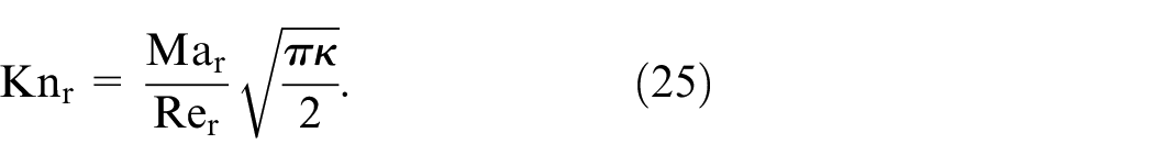
Due to the correlations (11) and (12), the exact expression for the relation between Reynolds number and the small parameter ε follows:

$${\mathrm{Re}}_{\mathrm{r}}=\frac{\beta }{\gamma }{\epsilon }^{\mathrm{m}-1}.$$

(26)

Furthermore, from the equation (25) with equations (10), (11), and (26) follow both the relation between the parameters β, γ, and η, and the relation between the parameters m and n:

$$\beta =\frac{{\gamma }^2\pi }{2{\eta }^2}\mathrm{and}2\mathrm{n}+\mathrm{m}=2.$$

(27)

Since we have considered slip and subsonic gas flow, the parameters m and n have to be positive (10), (11). These conditions, together with the relation (27) lead to the allowed limits for the parameters m and n: 0 < m < 2 and 0 < n < 1. Within these ranges, two characteristic problems follow from the equation (26):

1. Low Reynolds numbers gas flow, ²² where Re_r < 1, 1 < m < 2 and 0 < n < 1/2, and

2. Moderately high Reynolds numbers, where Re_r ≥ 1, 0 < m ≤ 1 and 1/2 ≤ n < 1.

The solution procedure is to expand the pressure, velocity, and temperature into a regular perturbation series^16–19:

$$\varphi ={\varphi }_0+\mathrm{K}{\mathrm{n}}_{\mathrm{r}}{\varphi }_1+{\mathrm{Kn}}_{\mathrm{r}}^2{\varphi }_2+O\left({\mathrm{Kn}}_{\mathrm{r}}^3\right)$$

and put them into the system of governing equations and boundary conditions (15)−(23) to get the systems of equations of the order O(1), O(Kn), O(Kn²)…. Here ϕ₀ corresponds to the solution for the flow with no-slip boundary conditions, and ϕ₁, ϕ₂, and the others comprise the corrections for the slip and temperature jump on the wall and other higher order effects.

In this paper, the more comprehensive solution, that is, the solution for moderately high Reynolds numbers is presented. The parameters m and n are chosen to be equal (m = n=2/3) to involve the rarefaction together with all the other second-order effects (inertia in the momentum equation, and the convection, dissipation, and rate at which work is done in compressing the element of fluid in the energy equation) in the second approximation. The dimensionless numbers in that case are: ${\mathrm{Re}}_{\mathrm{r}}=\frac{\beta }{\gamma }{\epsilon }^{-1/3}$ , $\kappa {\mathrm{Ma}}_{\mathrm{r}}^2=\beta {\epsilon }^{2/3}$ , $\mathrm{K}{\mathrm{n}}_{\mathrm{r}}=\eta {\epsilon }^{2/3}$ .

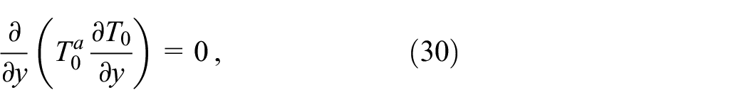
In this paper, the solution for pressure, velocity, and temperature is obtained by two approximations for moderately high Reynolds numbers. When the terms of the order O(1) and O(Kn_r) are extracted, the following two sets of equations and boundary conditions are obtained:

• O(1):

$$\frac{\partial (p_0{u}_0/T_0)}{\partial x}+\frac{\partial (p_0{V}_0/T_0)}{\partial y}=0,$$

(28)

$$\frac{\partial }{\partial y}\left(T_0^a\frac{\partial u_0}{\partial y}\right)=\frac{1}{\gamma }\frac{\mathrm{d}{p}_0}{\mathrm{d}x},$$

(29)

$$\frac{\partial }{\partial y}\left(T_0^a\frac{\partial T_0}{\partial y}\right)=0,$$

(30)

$${u_0|}_{y=0}=1,{V_0|}_{y=0}=0,$$

(31)

$${u_0|}_{y=h}=0,{V_0|}_{y=h}={u_0|}_{y=h}{\frac{\mathrm{d}h\left(x\right)}{\mathrm{d}x}|}_{y=h}=0,$$

(32)

$${T_0|}_{y=0}=T_{\mathrm{w}1}=1+\theta ,$$

(33)

$${T_0|}_{y=h}=T_{\mathrm{w}2}=1-\theta .$$

(34)

• O(Kn_r):

$$\frac{\partial }{\partial x}\underset{1+\theta }{\overset{1-\theta }{\int }}(p_0{u}_1{T}_0^{a-1}-p_0{T}_1{u}_0{T}_0^{a-2}+p_1{u}_0{T}_0^{a-1})\mathrm{d}{T}_0=0,$$

(35)

$$\begin{array}{c}\frac{\beta }{\gamma }\frac{p_0}{C_1^2}(u_0\frac{\partial u_0}{\partial T_0}\left(\frac{h\prime }{h}\right)(\frac{-T_0^a}{a+1}+\frac{C_2}{T_0})+\frac{C_1{V}_0}{T_0}\frac{\partial u_0}{\partial T_0})\hfill \\ =-\frac{T_0^a}{\gamma C_1^2}p{\prime }_1+\frac{\partial }{\partial T_0}(\frac{\partial u_1}{\partial T_0}+a\frac{T_1}{T_0}\frac{\partial u_0}{\partial T_0}),\hfill \end{array}$$

(36)

$$\begin{array}{c}\frac{\beta \mathrm{Pr}}{\gamma }\frac{p_0}{C_1^2}(u_0\left(\frac{h\prime }{h}\right)(\frac{-T_0^a}{a+1}+\frac{C_2}{T_0})+\frac{C_1{V}_0}{T_0})\hfill \\ =\frac{A}{\gamma C_1^2}{T}_0^a{u}_{0}p{\prime }_0+\frac{\partial }{\partial T_0}(a\frac{T_1}{T_0}+\frac{\partial T_1}{\partial T_0})+A{\left(\frac{\partial u_0}{\partial T_0}\right)}^2,\hfill \end{array}$$

(37)

$${u_1|}_{y=0}=\alpha T_{\mathrm{w}1}^{0.5}\frac{C_1}{p_0}((a+2)T_{\mathrm{w}1}^{(a+1)}b+C_3),{V_1|}_{y=0}=0,$$

(38)

$$\begin{array}{c}{u_1|}_{y=h}=-\alpha T_{\mathrm{w}2}^{0.5}\frac{C_1}{p_0}((a+2)T_{\mathrm{w}2}^{(a+1)}b+C_3),\hfill \\ {V_1|}_{y=h}={u_1|}_{y=h}{h\prime |}_{y=h},\hfill \end{array}$$

(39)

$${T_1|}_{y=0}=L{T}_{\mathrm{w}1}^{0.5}\frac{C_1}{p_0},$$

(40)

$${T_1|}_{y=h}=-L{T}_{\mathrm{w}2}^{0.5}\frac{C_1}{p_0},$$

(41)

where A, L, and α are constants defined as A = βPr (κ− 1)/ κ, L = 2κ(2 −σ_T)/(σ_T(κ+1)Pr), and α = (2 −σ_v)/σ_v.

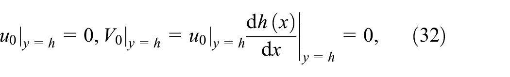
The solution procedure for both systems of equations is the same. First, the approximation of the temperature is derived from the corresponding energy equation (30, 37) along with the temperature boundary conditions (33, 34, 40, 41). Then, the approximation of the velocity is derived from the corresponding momentum equation (29, 36) and the velocity boundary conditions (31, 32, 38, 39). The pressure approximation follows from the continuity equation (28, 35). Finally, the analytical solutions for the first and second approximations for temperature and velocity in the microbearings with different temperatures of the walls and moderately high Reynolds numbers are respectively:

$$\begin{array}{c}{T}_0={\left[(a+1)(C_{1}y+C_2)\right]}^{\left(\frac{1}{a+1}\right)},\hfill \end{array}$$

(42)

$$\begin{array}{c}{u}_0={\mathrm{bT}}_0^{(a+2)}+C_3{T}_0+C_4,\hfill \end{array}$$

(43)

$$\begin{array}{c}\multicolumn{1}{c}{V_0={\mathrm{cT}}_0^{(2a+3)}+{\mathrm{dT}}_0^{(a+2)}+{\mathrm{eT}}_0^{(a+1)}+g{T}_0+i,}\end{array}$$

(44)

$$\begin{array}{c}\multicolumn{1}{c}{T_1=k_1{T}_0^{(2a+4)}+l{T}_0^{(a+3)}+m{T}_0^{(a+2)}+n{T}_0^2}\\ +o{T}_0+w{T}_0^{-a}+q{T}_0\ln T_0,\hfill \end{array}$$

(45)

$$\begin{array}{c}\multicolumn{1}{c}{u_1=f_1{T}_0^{(3a+5)}+f_2{T}_0^{(2a+4)}+f_3{T}_0^{(2a+3)}+f_4{T}_0^{(a+3)}}\\ +f_5{T}_0^{(a+2)}+f_6{T}_0^{(a+1)}+f_7{T}_0^2+f_8{T}_0\hfill \\ +f_9{T}_0^{-a}+f_{10}{T}_0^{(a+2)}\ln T_0+f_{11}{T}_0\ln T_0+f_{12},\hfill \end{array}$$

(46)

where C_i, f_j, (i = 1,2…6; j = 1,2…12) C_c1, C_c3, C_c4, b, c, d, e, g, i, k₁, l, m, n, o, w, and q are given in the Appendix.

Both approximations for pressure along the microbearing are the solutions of the two second-order differential equations:

$$\left(h^3{p}_0{p\prime }_0\right)\prime +C_c\left(h{p}_0\right)\prime =0,$$

(47)

$$\begin{array}{c}\left(\frac{p_0{p\prime }_1}{C_1^3}\right)\prime b_c{C}_{c1}^3(\frac{(T_{\mathrm{w}2}^{(a+1)}+T_{\mathrm{w}1}^{(a+1)})}{2}+\frac{C_{c3}}{b_c}-\frac{(a+1)T_{\mathrm{w}1}{T}_{\mathrm{w}2}(T_{\mathrm{w}2}^a-T_{\mathrm{w}1}^a)}{a(T_{\mathrm{w}1}-T_{\mathrm{w}2})})\hfill \\ +\left(\frac{b{p}_1}{C_1}\right)\prime \frac{T_{\mathrm{w}2}^{(2a+2)}-T_{\mathrm{w}1}^{(2a+2)}}{2(a+1)}+C_{c1}\left(\frac{C_3{p}_1}{C_1}\right)\prime +\left(\frac{C_4{p}_1}{C_1}\right)\prime \frac{T_{\mathrm{w}2}^a-T_{\mathrm{w}1}^a}{a}\hfill \\ +\left(\frac{p_0(f_1-b{k}_1)}{C_1}\right)\prime \frac{T_{\mathrm{w}2}^{(4a+5)}-T_{\mathrm{w}1}^{(4a+5)}}{(4a+5)}+\left(\frac{p_0(f_2-C_3{k}_1-bl)}{C_1}\right)\prime \frac{T_{\mathrm{w}2}^{(3a+4)}-T_{\mathrm{w}1}^{(3a+4)}}{(3a+4)}\hfill \\ +\left(\frac{p_0(f_3-C_4{k}_1-bm)}{C_1}\right)\prime \frac{{T_{\mathrm{w}2}}^{(3a+3)}-{T_{\mathrm{w}1}}^{(3a+3)}}{(3a+3)}+\left(\frac{p_0(f_6-C_{4}m)}{C_1}\right)\prime \frac{T_{\mathrm{w}2}^{(2a+1)}-T_{\mathrm{w}1}^{(2a+1)}}{(2a+1)}\hfill \\ +\left(\frac{p_0(f_4-C_{3}l-bn)}{C_1}\right)\prime \frac{{T_{\mathrm{w}2}}^{(2a+3)}-{T_{\mathrm{w}1}}^{(2a+3)}}{(2a+3)}+\left(\frac{p_0(f_7-C_{3}n)}{C_1}\right)\prime \frac{T_{\mathrm{w}2}^{(a+2)}-T_{\mathrm{w}1}^{(a+2)}}{(a+2)}\hfill \\ -\left[\frac{p_0}{C_1}(\frac{(5a+8)f_{10}}{2(a+1)(a+2)}+\frac{f_{99}}{(a+1)(a+2)}+C_{3}m+C_{4}l+b(o-\frac{q}{2(a+1)}))\right]\prime \hfill \\ \frac{T_{\mathrm{w}2}^{(2a+2)}-T_{\mathrm{w}1}^{(2a+2)}}{2(a+1)}+\left(\frac{p_0(f_{10}-\mathrm{bq})}{C_1}\right)\prime \left(\frac{T_{\mathrm{w}2}^{(2a+2)}\ln T_{\mathrm{w}2}-T_{\mathrm{w}1}^{(2a+2)}\ln T_{\mathrm{w}1}}{2(a+1)}\right)\hfill \\ +\left[\frac{p_0}{C_1}(C_{88}+C_4(\frac{q}{a}-o))\right]\prime \frac{T_{\mathrm{w}2}^a-T_{\mathrm{w}1}^a}{a}+\left(\frac{C_{4}w{p}_0}{C_1}\right)\prime ({T_{w2}}^{-1}-{T_{w1}}^{-1})-\left(\frac{p_0{C}_{4}q}{C_1}\right)\prime \hfill \\ +C_{c1}\left[\frac{p_0}{C_1}(C_{77}-f_{11}\frac{a+2}{a+1}-C_{4}n-bw+C_3(\frac{q}{a+1}-o))\right]\prime \hfill \\ \frac{T_{\mathrm{w}2}^a\ln T_{\mathrm{w}2}-T_{\mathrm{w}1}^a\ln T_{\mathrm{w}1}}{a}+\left(\frac{p_0(f_{11}-C_{3}q)}{C_1}\right)\prime \frac{T_{\mathrm{w}2}^{(a+1)}\ln T_{\mathrm{w}2}-T_{\mathrm{w}1}^{(a+1)}\ln T_{\mathrm{w}1}}{(a+1)}=0,\hfill \end{array}$$

(48)

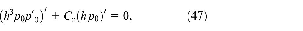
where ′ denotes the derivative with respect to x, while f₉₉, C₇₇, C₈₈ are given in the Appendix. There are four boundary conditions for pressure approximations at the microbearing’s inlet and outlet that are satisfied: ${p_0|}_{x=0}={p_0|}_{x=1}=1$ and ${p_1|}_{x=0}={p_1|}_{x=1}=0$ .

The velocity, temperature, and pressure analytical solutions derived for different temperature walls microbearings gas flow and the moderately high Reynolds numbers are:

$$\begin{array}{c}\multicolumn{1}{c}{u=u_0+\mathrm{K}{\mathrm{n}}_{\mathrm{r}}{u}_1}\\ =b{T}_0^{(a+2)}+C_3{T}_0+C_4+\mathrm{K}{\mathrm{n}}_{\mathrm{r}}\hfill \\ (f_1{T}_0^{(3a+5)}+f_2{T}_0^{(2a+4)}+f_3{T}_0^{(2a+3)}+f_4{T}_0^{(a+3)}\hfill \\ +f_5{T}_0^{(a+2)}+f_6{T}_0^{(a+1)}+f_7{T}_0^2+f_8{T}_0+f_9{T}_0^{-a}\hfill \\ +f_{10}{T}_0^{(a+2)}\ln T_0+f_{11}{T}_0\ln T_0+f_{12}),\hfill \end{array}$$

(49)

$$\begin{array}{c}T=T_0+{\mathrm{Kn}}_{\mathrm{r}}{T}_1\\ =T_0+{\mathrm{Kn}}_{\mathrm{r}}(k_1{T}_0^{\left(2a+4\right)}+l{T}_0^{\left(a+3\right)}+m{T}_0^{\left(a+2\right)}+n{T}_0^2+o{T}_0+w{T}_0^{-a}+q{T}_0\ln T_0),\end{array}$$

(50)

$$\begin{array}{c}p=p_0+\mathrm{K}{\mathrm{n}}_{\mathrm{r}}{p}_1,\hfill \end{array}$$

(51)

where T₀ is defined by the equation (42), k₁, l, m, n, o, w, q, and f_i (i = 1,2…12) are given in the Appendix, and p₀ and p₁ are the solutions of the differential equations (47) and (48).

Based on the presented solution, it is now possible to determine different physical properties. From the solution for the continuum (42, 43, 47) and slip (49)−(51), the non-dimensional mass flow rates through microbearings for the continuum and slip flow can be calculated respectively:

$${\stackrel{·}{m}}_0=\underset{0}{\overset{1}{\int }}\frac{p_0}{T_0}{u}_0\mathrm{d}y,$$

(52)

$$\stackrel{·}{m}=\underset{0}{\overset{1}{\int }}\frac{p}{T}u\mathrm{d}y.$$

(53)

Furthermore, the non-dimensional load carrying capacity for the continuum and slip gas flow are respectively:

$$w_0=\underset{0}{\overset{1}{\int }}(p_0-1)\mathrm{d}x,$$

(54)

$$w=\underset{0}{\overset{1}{\int }}(p-1)\mathrm{d}x.$$

(55)

Results, discussion, and verification

In gas slide microbearings, the lubricant is a gas between a moving and a steady wall. Hence, the gas flow is shear-driven. The forces act upon the walls of the microbearing, tending to push them together. Because of that, the gas layer must develop normal stresses, above all the pressure, which carries the load. Thus the first goal of lubrication theory is to predict the pressure distribution and, based on it, the load-carrying capacity. After that, it relates the velocity to the pressure gradient. By the presented method, we involve inertia as the second-order effect in the momentum equation. We have obtained the temperature field (which, for different walls’ temperatures, is defined primarily by conduction) by adding convection and dissipation rate at which work is done in compressing the element of fluid in the energy equation. The included dependence of the dynamic viscosity and thermal conductivity on temperature makes the velocity and temperature fields coupled.

That way, the results for the pressure, velocity, and temperature fields (49)−(51) for different walls’ temperature microbearing gas flow is going to be presented and analyzed. The dimensional analysis of the problem shows that five dimensionless quantities (parameters) are necessary and sufficient to define it completely. For the presentation of the results we have selected: the reference Knudsen and Mach numbers, half of the dimensionless temperature difference between the lower and upper walls θ, the bearing number $\mathrm{\Lambda }$ , and the ratio between the inlet and exit microbearing heights $h_{\mathrm{i}}$ . That way, it is possible to present and analyze the influence of those parameters on the pressure, velocity, and temperature fields. All the results correspond to the diffuse reflection, so σ _v  = 1, σ _T  = 1, and to a monatomic gas, thus κ = 5/3 and Pr = 2/3 (Prandtl number for monatomic gases varies little with temperature, but is nearly equal to 2/3).^2,21

Unlike in our previous work, ¹⁹ where the transport coefficients were taken as constant (the temperature influence on them was neglected), here we consider the dependence of the dynamic viscosity and thermal conductivity on the temperature (13). Because of that, the results could be presented for different values of the viscosity-temperature index a, which takes values 0 (dependence of the temperature on transport properties is neglected) and from 0.5 for the elastic sphere molecule model to 1 for the Maxwellian molecules.

Figures 2 and 3 present the influence of the transport coefficients’ dependence on the temperature for bearing numbers Λ = 1 and Λ = 100, respectively. Both figures show the presented solution for pressure distribution for continuum (dotted line) and slip gas flow at Kn_r = 0.1 (full line) for several viscosity-temperature indexes a and θ = 0.5, h_i = 2. The continuum corresponds to the higher pressure values along the microbearing for all values of a. If we neglect the dependence of the viscosity-temperature index on the temperature (a = 0), the pressure distribution is underestimated in both continuum and slip regime (lines without symbols). Furthermore, the higher value of index a corresponds to the higher pressure along the microbearing regardless of the value of the bearing number Λ and moves the position of the pressure maximum slightly to the bearing exit (Figure 3(b)).

Figure 2.

Pressure distribution for continuum (47) and slip flow (51) (Kn_r = 0.1, Ma_r = 0.3) along the microbearing for: θ = 0.5, Λ = 1, h_i = 2 and different viscosity-temperature indexes a.

Figure 3.

(a) Pressure distribution for continuum (47) and slip flow (51) (Kn_r = 0.1, Ma_r = 0.3) along the microbearing for: θ = 0.5, Λ = 100, h_i = 2 and different viscosity-temperature indexes a; (b) the detail from (a) enlarged.

Figures 4 and 5 show the influence of the reference Mach number on the pressure distribution along the microbearing. Figure 4 corresponds to Λ = 1, and Figure 5 to Λ = 100. It is evident that for the same rarefaction (Kn_r = 0.1), the higher Ma_r leads to the higher pressure, that is, load carrying capacity of the microbearing. The analysis shows that with Ma_r decreasing, discrepancies between the results obtained by the presented model that include all second-order effects, and the results that include only rarefaction as the second-order effect, ²² decreases. It means that for small reference Mach numbers (Ma_r ≤ 0.1) we can use the solution by Milićev and Stevanović ²² that comprises only rarefaction as the second-order effect.

Figure 4.

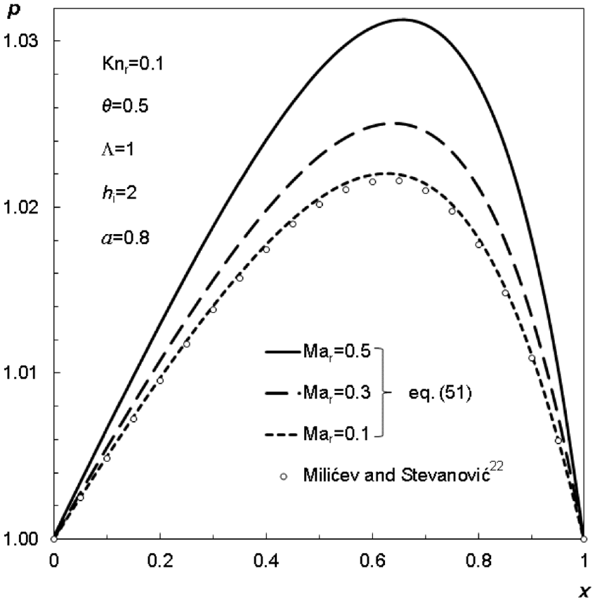
Pressure distribution for slip flow (51) (Kn_r = 0.1) along the microbearing for: θ = 0.5, Λ = 1, h_i = 2 for different Ma_r.

Figure 5.

(a) Pressure distribution for slip flow (51) (Kn_r = 0.1) along the microbearing for: θ = 0.5, Λ = 100, h_i = 2 and a = 0.8, for different Ma_r; (b) the detail from (a) enlarged.

Figure 6 presents the velocity and temperature in the inlet and outlet cross sections of the microbearing for h_i = 2, θ = 0.5, Λ = 1, and two viscosity-temperature indexes, a = 0 (constant transport coefficients) and the maximal value a = 1. Figure 6(a) shows the results of the presented model for the continuum and Figure 6(b) for the slip flow (Kn_r = 0.1, Ma_r = 0.3). The continuum is without temperature jump and slip on the walls, and without any second-order effects (rarefaction, inertia, convection, dissipation, and the rate at which work is done in compressing the element of fluid). The velocity for the continuum increases from the inlet to the outlet cross section in both the continuum and slip regimes, while the first approximation for the temperature (continuum), presented in Figure 6(a), remains unchanged along the microbearing. For the continuum and constant thermal conductivity k, the presented model gives the linear temperature profile (equation (42) for a = 0). Figure 6(b) shows that the velocity slip and temperature jump increase, as well as the velocity over the cross section toward the microbearing exit.

Figure 6.

The velocity and temperature in the inlet and outlet cross section of the microbearing for h_i = 2, θ = 0.5, Λ = 1 and two viscosity-temperature indexes, a = 0 and a = 1; (a) continuum and (b) slip flow (Kn_r = 0.1, Ma_r = 0.3).

Figure 7 presents the velocity in the inlet and outlet cross sections of the microbearing for Λ = 100 and h_i = 2, θ = 0.5. The conclusions are qualitatively the same in both the continuum and slip domains as for the velocity field presented in Figure 6. The higher values of the velocity correspond to higher values of the bearing number Λ (Figure 7). The presented velocity and temperature profiles in Figures 6 and 7 show that constant transport coefficients (lines without symbols) underestimate both the velocity and temperature in the entire microbearing gas field.

Figure 7.

The velocity in the inlet and the outlet cross sections of the microbearing for h_i = 2, θ = 0.5, Λ = 100, and two viscosity-temperature indexes, a = 0 and a = 1; (a) continuum and (b) slip flow (Kn_r = 0.1, Ma_r = 0.3).

The influence of the reference Mach number values on the velocity and temperature fields for bearing numbers Λ = 1 and Λ = 100 are presented in Figures 8 and 9, respectively. The results correspond to Kn_r = 0.1, h_i = 2, θ = 0.5, a = 0.8, and three different reference Mach number values: Ma_r = 0.1, Ma_r = 0.3, and Ma_r = 0.5. For the same rarefaction (Kn_r = 0.1), the influence of the second-order effects is higher for higher Ma_r. For determining the velocity and temperature, the same as for pressure for small reference Mach numbers (Ma_r ≤ 0.1), we can use the solution which comprises only rarefaction as the second-order effect. ²²

Figure 8.

The velocity for slip flow in the inlet and the outlet cross sections of the microbearing for Kn_r = 0.1, h_i = 2, θ = 0.5, a = 0.8, for different Ma_r and for: (a) Λ = 1 (b) Λ = 100.

Figure 9.

The temperature for slip flow in the inlet and the outlet cross sections of the microbearing for Kn_r = 0.1, h_i = 2, θ = 0.5, a = 0.8, for different Ma_r and for: (a) Λ = 1 (b) Λ = 100.

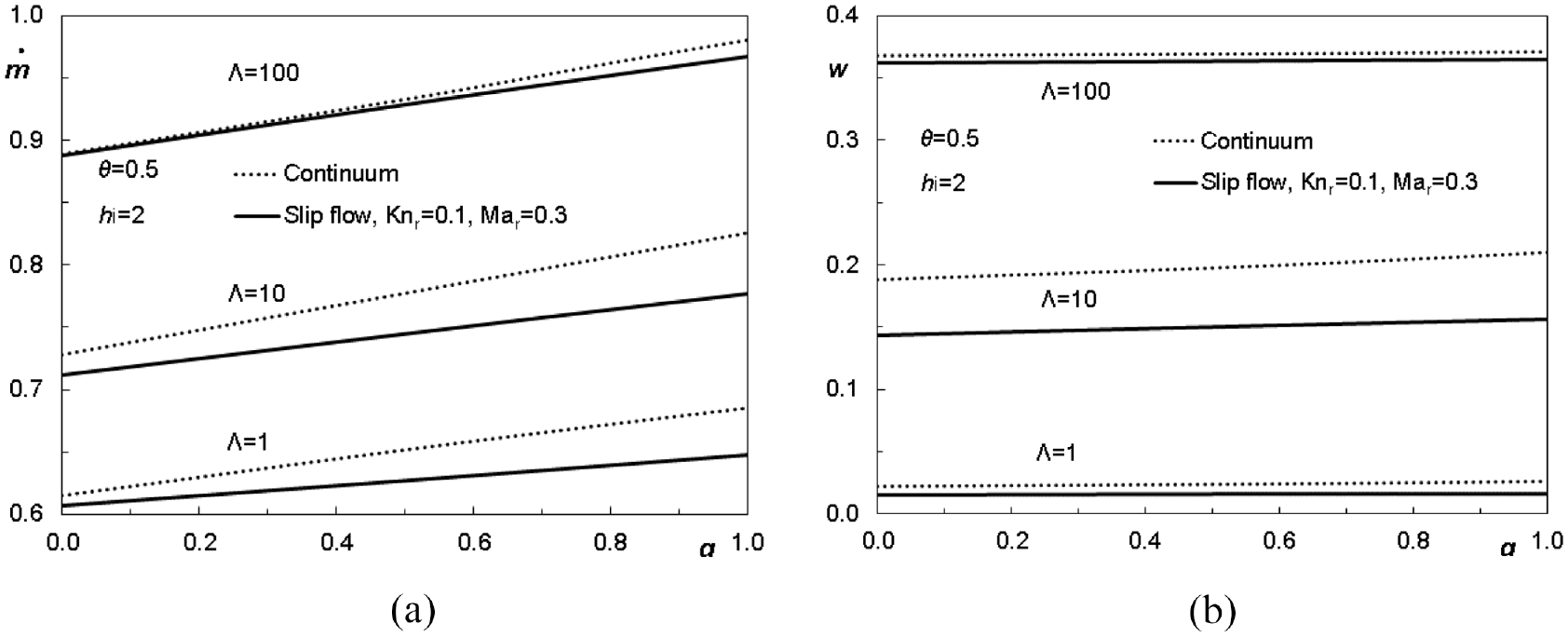
The cumulative effect of the velocity field, that is, mass flow rate, is even more interesting. Based on the presented results for pressure, velocity and temperature, the calculations of the mass flow rate for the continuum (52) and for the slip domain (53) show that neglecting the dependence of the viscosity-temperature index on the temperature produces an error. If the mass flow rate is calculated with a = 0, its underestimation cannot be negligible. For Λ from 1 to 100, it is up to 9% in the case of slip flow, while it is up to 12% for the continuum. Figures 10(a) and 11(a) show the influence of the values of the index a on the mass flow rates for microbearings with different bearing numbers.

Figure 10.

Dependence of (a) the mass flow and (b) load carrying capacity on bearing number for different viscosity-temperature indexes and h_i = 2, θ = 0.5; the flow is continuum and slip (Kn_r = 0.1, Ma_r = 0.3).

Figure 11.

Dependence of (a) the mass flow and (b) the load carrying capacity on the viscosity-temperature index for different bearing numbers and h_i = 2, θ = 0.5; the flow is continuum and slip (Kn_r = 0.1, Ma_r = 0.3).

The pressure increases with the increase of the viscosity-temperature index. Even though that pressure increment is up to 1% in the case of bearing number Λ = 1 (Figure 2) when viscosity-temperature index increases from a = 0 to a = 1, the cumulative effect is much higher. The load carrying capacity (54, 55), increases up to 6% in the case of the slip gas flow and up to 15% for the continuum, Figures 10(b) and 11(b). For microbearing with bearing number Λ = 100 the influence of the viscosity-temperature index on the load carrying capacity is almost negligible.

In addition, as a confirmation of the model, we present a comparison with the results of Doi. ¹⁵ Figure 12 shows the velocity profiles in the mid cross-section (x = 0.5) with equal (θ = 0) and different walls’ temperatures (θ = 0.33, i.e. ${\tilde{T}}_{w1}=2{\tilde{T}}_{w2}$ ). The temperature profiles in three microbearing’s cross-sections are compared with the results of the same author in Figure 13. The good agreement in the velocity and temperature fields confirms the presented analytical results as reliable. Besides, as it has been shown so far, our results are repeatable and easy for application for a variety of parameters that define lubrication flow in microbearings.

Figure 12.

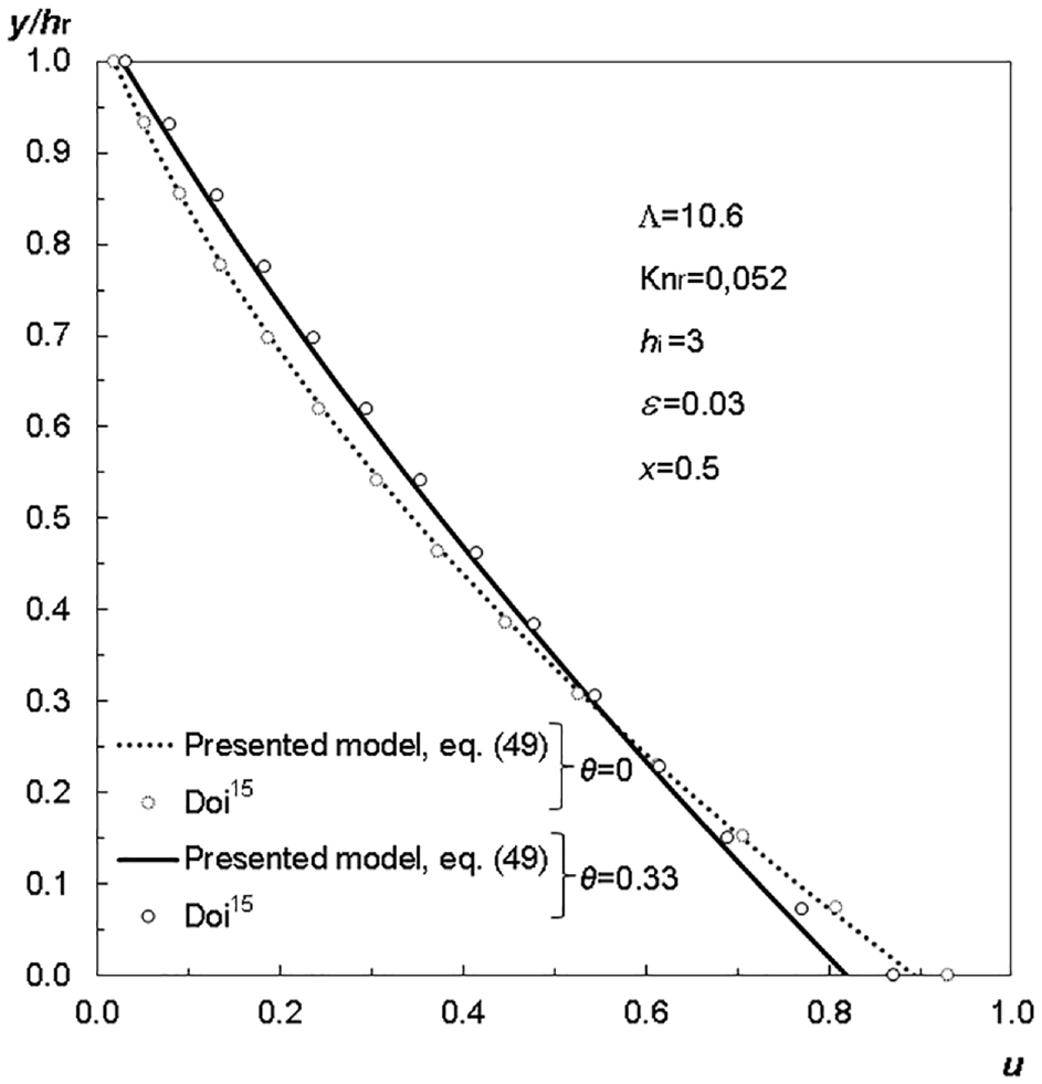
Comparison of the presented results for the velocity (49) in x = 0.5 cross-section of microbearing with equal (θ = 0) and different (θ = 0.33) walls’ temperatures with those of Doi ¹⁵ ; (Λ = 10.6, Kn_r = 0.052, h_i = 3, and ε = 0.03).

Figure 13.

Comparison of the presented results for the temperature (50) in cross-sections x = 0.1, x = 0.5, and x = 0.98 of microbearing with equal (θ = 0) walls’ temperatures with those of Doi ¹⁵ ; (Λ = 10.6, Kn_r = 0.052, h_i = 3, and ε = 0.03).

Conclusions

The presented perturbation method makes it possible to obtain a non-isothermal analytical solution for a shear-driven gas flow in microbearings for different walls’ temperatures and moderately high Reynolds numbers. However, the method is applicable wider, for the gas flow in microchannels with steady or moving walls, micropipes, etc.

Two approximations of the pressure, velocity, and temperature have been defined in terms of perturbation series. The first one corresponds to the continuum flow conditions, while the second one represents the contribution of the second-order effects: rarefaction, inertia, convection, dissipation, and rate at which work is done in compressing the element of fluid. The explicit solution of the pressure, velocity, and temperature fields enable analyses of the influence of different variables on the results. The rarefaction causes a lower pressure in the microbearing, while the other second-order effects have the opposite impact, increasing the pressure in the microbearing. The rarefaction leads to the velocity slip and temperature jump on both walls, which increases from the inlet to the outlet of the microbearing. The second-order effects have the influence on the entire velocity and temperature profiles, too.

In this paper, the attention has been especially focused on the influence of the viscosity-temperature index a on the solution for pressure, velocity, and temperature. The hard sphere molecular model is used to shape the dynamic viscosity and heat conductivity dependence on the temperature. The index a takes values from a = 0.5 for the elastic sphere molecule model, to a = 1 for the Maxwellian molecules. Assuming that the transport coefficients are independent of temperature (a = 0), that is, they are constant, underestimation arises in all three fields: velocity, temperature, and pressure, and accordingly, in the load carrying capacity and mass flow rate. It is shown that the error cannot be neglected, since the mass flow rate can be smaller up to 12%, while the capacity can be smaller up to 15%, depending on the values of the viscosity-temperature index and the bearing number.

The validation of the presented results by those obtained by Doi ¹⁵ make our results reliable. Besides, as there are analytical, they can be used in research of the influence of a variety of parameters that define lubrication flow in microbearings.