Sage Journals: Discover world-class research

Abstract

The application of industrial robots in the field of machining is gradually increasing, but their low absolute position accuracy and low stiffness affect the improvement of machining accuracy. Computer numerical control (CNC) has good performance to control the motion accuracy in the machine tool. Therefore, it is proposed to improve the motion accuracy of robots. This article utilizes a stereo high-speed camera to track robot motion. Circular paths running under the CNC system are planned to evaluate its performance, which includes path accuracy, motion velocity, and acceleration. The performance of identical paths running in a conventional robot controller is evaluated for comparison. Based on the experimental analysis, the CNC system, which has more functionalities for acceleration regulation, can get better path accuracy and stability. It indicates that acceleration control has a significant effect on path accuracy and motion velocity. The acceleration profile in a conventional robot controller resembles a triangle. By default, the maximum acceleration value is adopted for the motion planning. Therefore, its accelerating and decelerating phase is much shorter than that of the CNC system, which could lead to instability. Both Step-shaped and trapezoidal acceleration profiles in the CNC system improve the dynamic behavior of the robot. Considering the trade-off between path accuracy and motion velocity, the Step-shaped acceleration profile can be applied to the optimization of the traditional robot motion control.

Keywords

Industrial robot CNC motion control dynamics

Introduction

As an important process in the manufacturing process,¹ machining is mainly completed by using CNC machine tools with high precision and good stability. Compared to CNC machine tools, industrial robots have low cost, good flexibility, and large workspace, and they are gradually favored by the manufacturing industry. It can replace the traditional CNC machine tools to complete part of the machining tasks. At present, the main machining processing can be realized by industrial robots, include milling, drilling, grinding, cutting, deburring, polishing, and friction stir welding. The involved industries include aerospace, automobile manufacturing, casting, medical treatment, plastics, and wood processing.^2–4 Especially in the machining of large-scale component, industrial robots are more efficient than the machine tool, for example, drilling holes on the Inboard Flaps⁵ and milling operation for a windmill.⁴ Although industrial robots have advantages, two major factors affect the accuracy of robotic machining. One factor is the low absolute position accuracy. Industrial robots have high position repeatability, for example, the KUKA KR210 industrial robot, which has a payload of 210 kg, can reach position repeatability with ±0.06 mm. However, the absolute position accuracy in the entire workspace is approximately ±3 mm.⁶ Another factor is the low stiffness, which results in unexpected deformation and vibration/chatter during the machining process.^7,8 The cutting force of 500 N introduces a position error of 1 mm to the robot, while the error introduced to the CNC machine tool is less than 0.01 mm.^9,10

To improve the accuracy of robotic machining, two main approaches are studied to overcome the above problems. The first approach is the optimization of the structure of industrial robots. Sun et al.¹¹ developed a novel industrial robot, whose structure is specially designed to enhance its stiffness. The manufacturers of industrial robots also produce industrial robots for machining tasks. For example, ABB produces the IRB 6660 for press tending and machining, which has an additional parallel arm to make the robot stiffer and special dual bearing design to overcome the fluctuating process forces in machining.¹² KUKA offers KR 500 FORTEC MT (Machining Tooling), which is predestined for milling applications in the high payload range.¹³

Another approach is to improve the control system. The optimization of the robot structure can improve the entire stiffness of the robot, but the nonlinearity distribution of the stiffness is an intrinsic characteristic of industrial robots. To achieve the accuracy requirement of some machining applications, the stiffness model is established to integrate in the robot control system for the deformation compensation. Based on the stiffness model, the deformation resulting from the machining forces can be calculated from the force data and robot position.^14–17 In addition to the integration of the stiffness model, an external sensor system is adopted to compensate the position in real time. Kubela et al. apply the online path compensation using a laser tracker on a KUKA robot for the milling task. Real position data are first processed with an industrial PC and subsequently transferred into the robot controller. Through the KUKA RSI (Robot Sensor Interface), the robot position is compensated in 4 ms, which improves the part accuracy by approximately 15%–20%.¹⁸ A similar approach was adopted by other researchers.^19,20 RC (robot control) considered not only the motion control but also the interface to communicate with an external sensor system according to the specific robot from different manufacturers. As RC is machine-related, specialized robot functions can be provided, which have the advantage of quickly programming the handling and automation tasks.²¹ For the machining process, the movement strategies are completely different. The Computerized Numerical Control (CNC) system, which has the advantage of high-accuracy manufacturing, short production time, and greater manufacturing flexibility, has been widely used in machine tools. Therefore, CNC is selected for robot motion control by robot manufacturers. For example, MABI Robotic company has directly used CNC SINUMERIK 840D sl from Siemens as the robot control system for the type Max 100.²² KUKA company has integrated two types of CNC kernels into its robot control system.^21,23

To determine the performance of the robot motion under the control of the CNC kernel, this article focuses on the dynamic performance of the robot when it runs circular paths. The parameters that plan the trajectory in two control systems are discussed. Experiments are designed based on the comparison of two control systems. The robot motions are tracked with a high-speed stereo camera system. Influences of the key parameters on the path accuracy and dynamic behavior are investigated based on experimental analysis.

Control system

Current robot controls mainly use cascaded controls, as shown in Figure 1. The robot trajectory is normally planned in the operational space of the robot. Based on the inverse mathematical model of the robot, the trajectory planning generates position values with corresponding angular velocity and angular acceleration in the joint space. Each axis is described as a single-input single-output system with internal current control cascade, speed control cascade, and outer position control cascade.²⁴

Figure 1.

Standard robot cascade control.

Due to the errors of the model and disturbances from driving systems,²⁵ differences can appear between target value and actual value. Therefore, feedback control is formed to compensate the errors based on the measuring data from the sensors, which are encoders installed on the motor side. There is normally only one primary encoder for each joint. When the required robot accuracy increases, an additional secondary encoder is proposed to integrate into the output side of every joint.^5,26 The deformation and gear backlash in the driving system, which cannot be recognized by the primary encoder, can be measured by the secondary encoder. Thus, the position accuracy can be improved when double encoders are implemented in the control system. Möller et al.²⁴ adopted a CNC-based robotic system with the integration of a secondary encoder to enhance the machining accuracy of the large-scaled CFRP-Parts. The CNC control enables the users with no experience of robot control system to use the system. Furthermore, it provides advanced software modules that enable custom adjustments for machining operations. KUKA provides two types of CNC kernels: KUKA.CNC and KUKA.CNC Sinumerik. This paper investigates the practical performance of KUKA.CNC when the robot runs a circular path. This CNC kernel was developed by ISG (Industrielle Steuerungstechnik GmbH). It runs parallel to the KR C4 and has its own user interface. These two controllers have their own program languages. KUKA Robot Language (KRL) running on the KR C4 offers two types of programming forms, which are the user group (inline forms) and the expert group (KRL syntax). KUKA.CNC executes DIN 66025-compliant CNC programs. The complete standard code can be interpreted and implemented by the robot. However, the CNC mode should be activated by the KRL program before running the CNC program. The KRL function DEF gCodeExecute (GCodeFileName:IN) can be used for this purpose.^27,28

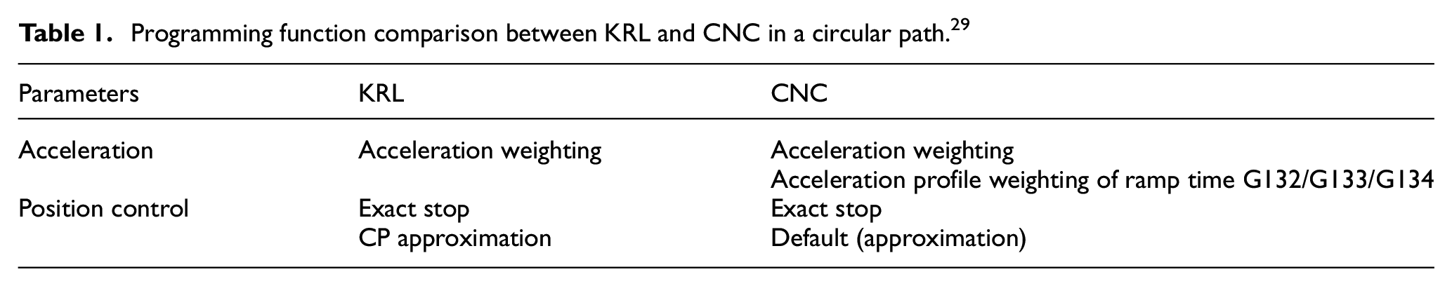
These two control systems have different functions in programming. As shown in Table 1, the major difference between two control systems is the control of the acceleration. CNC provides three types of acceleration profiles: step-shaped, trapezoidal, and square-sinusoidal profiles (Figure 2). The corresponding nomenclatures in CNC programs are Profile 0, Profile 1, and Profile 2.²⁹ In addition, the CNC kernel offers functions to regulate the ramp time of the axis acceleration. With the function G132/G133, it is possible to change the ramp time of the axis acceleration for Profile 1 and Profile 2 (Figure 3). G132 defines the weight in percentage for specific axes. G133 defines the weight in percentage for all axes. With function G134, the geometrical ramp time of the axis acceleration can be changed. During the programming of G132/G133/G134, nonprogrammed axes are set to the default value of 100%. As shown in Figures 3 and 4, the ramp time increases when the percentage increases. KRL has no option to select the acceleration profile. Experimental tests show that KRL has a default acceleration with the parabolic profile.³⁰

Table 1.

Programming function comparison between KRL and CNC in a circular path.²⁹

Parameters	KRL	CNC
Acceleration	Acceleration weighting	Acceleration weighting
		Acceleration profile weighting of ramp time G132/G133/G134
Position control	Exact stop	Exact stop
	CP approximation	Default (approximation)

Figure 2.

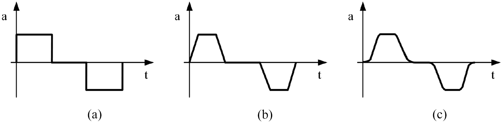
Acceleration profiles in CNC: (a) step-shaped (Profile 0), (b) trapezoidal (Profile 1), and (c) square-sinusoidal (Profile 2).

Figure 3.

Example for weighting of the ramp time with function G132/G133.

Figure 4.

Example for weighting of the ramp time with function G134 at circular interpolation.

Experiment

Based on the above comparison of programming systems, a group of circular paths, which are usually implemented with the telescopic ballbar to assess the performance of CNC machine tools, are planned for the analysis of the two robot control systems. A high-speed stereo camera system is used to track the motion of the robot. Details are introduced as follows.

Experimental design

According to the difference of the programming system in CNC and KRL, the experiments are planned in three aspects: (i) comparison between KRL path and CNC path, (ii) influence of acceleration profiles on the path accuracy in CNC, and (iii) influence of the change in ramp time and acceleration weighting on the path accuracy. To compare two control systems, the parameters of geometric shape of the paths and programmed velocity should be identical. In addition, similar acceleration values and acceleration profiles for two control systems should be planned. Based on a pretest study on acceleration, the velocity is set to 150 mm/s, and the radius is set to 50 mm. Two acceleration weights are set to 100% and 50% (Table 2). The experimental analysis indicates that the effect of acceleration Profile 1 and Profile 2 on a linear path is minimum.³¹ Therefore, Profile 0 and Profile 1 are selected for the experiment. For the circular path interpolation, the ramp time is regulated for all axes with two types of functions: G133 and G134. The specific data are stated in Table 2. All circular paths are programmed in the clockwise direction. The center of circular path is located at approximately (477, 1260, and 876 mm) with respect to the base coordinate system of the robot and lies in the YZ plane.

Table 2.

Parameters in the circular path program.

Group	Type	Velocity (mm/s)	Acceleration weighting (%)	Radius (mm)
1	KRL	150	50, 100	50
2	Profile 0	150	50, 100	50
3	Profile 1	150	50, 100	50
4	Profile 1, G133 = 10%	150	100	50
	Profile 1, G134 = 10%	150	100	50

Experiment setup

The experiment setup includes a KUKA robot, a metrology system, a testing tool, and a reference object, which are illustrated in Figure 5.

Figure 5.

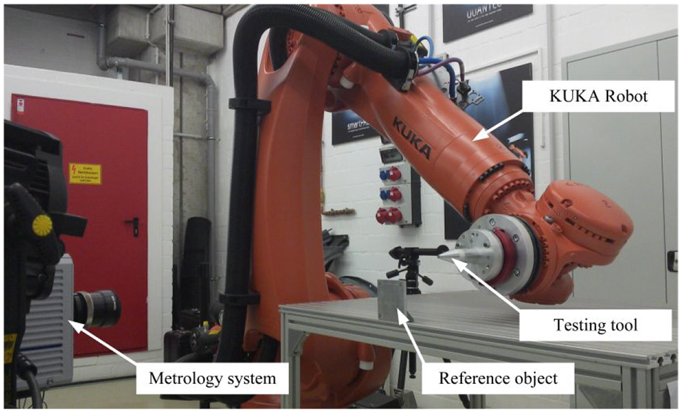
Experiment configuration.

The KUKA robot (KR 210 R2700) with six axes to be tested has a rated payload of 210 kg and a maximum reach of 2700 mm, whose position repeatability can reach ±0.06 mm.

The metrology system is a 3D high-speed camera measuring system named PONTOS. The maximum frame rate can reach 86,400 Hz with the corresponding camera resolution of 256 × 32 pixels. When the resolution increases, the frame rate correspondingly decreases. The maximum camera resolution is up to 2048 × 2048 pixels with a frame rate of 1080 Hz. Depending on the measuring area, its accuracy can reach 0.001 mm. The practical tests showed the accuracy of the measuring system: X = 0.0016 mm, Y = 0.0019 mm, and Z = 0.0051 mm. Since the Z direction is positioned in the direction of the focal depth axis, it has a relatively lower accuracy.³⁰ The testing tool, whose center is marked with a marker, is calibrated for the path programming. By identifying the marker, the metrology system can track the robot motion. The 3D coordinate values combined with the corresponding time are generated from the identified markers through the processing of the PONTOS software.³² As illustrated in Figure 6, markers are also marked on the reference object to build a reference coordinate system for the robot. This setup is aimed to eliminate the effect of the position change of the metrology system on the measuring accuracy. Based on the parameters designed for circular paths, a resolution of 2048 2048 pixels with the frame rate of 250 Hz is set in the measuring system for this experiment. Robot performance is also affected by temperature, working conditions, and kinematic model error. To reduce these errors, the robot has been calibrated and run for an hour before the measurement. The details of the measuring procedure were introduced in the previous article.³⁰

Figure 6.

Measurement markers and reference coordinate system: (a) measuring objects with markers and (b) identified tool center and reference coordinate system in the PONTOS software.

Experiment results and analysis

According to the experiment plan, the circular paths are performed in two control systems. The 3D coordinate values along the time series are measured using the metrology system. The experiment results are discussed in terms of the velocity, acceleration, and path accuracy. Because there are noises in the measuring data, an adaptive window filter similar to the end-fit filter in Janabi-Sharifi et al.³³ is used to process the measuring data to obtain the distribution of the velocity and acceleration. Instead of calculating backward differences, the filter windows are placed symmetrical. The distribution of velocity and acceleration of the circular paths are illustrated in Figures 7 –9.

Figure 7.

Velocity and acceleration distributions in circular paths of KRL: (a) velocity distribution and (b) acceleration distribution.

Figure 8.

Velocity and acceleration distributions in circular paths of CNC Profile 0: (a) velocity distribution and (b) acceleration distribution.

Figure 9.

Velocity and acceleration distributions in circular paths of CNC Profile 1: (a) velocity distribution and (b) acceleration distribution.

First, the experiment results of Group 1, Group 2, and Group 3 are discussed. Not all programmed paths can reach the programmed velocity. The acceleration values are different according to each type of paths. The average velocity in the steady phase and the maximum acceleration are obtained (Table 3). Both KRL path and Profile 0 path can reach the programmed velocity. The velocity in the steady phase indicates that the KRL path has more deviation from the programmed velocity than the Profile 0 path. The ratios of the deviation relative to the programmed velocity are approximately 1.1% and 0.1%. When the acceleration weight is reduced to 50%, the time to reach the programmed velocity increases. However, the CNC path takes more time than the KRL path to reach the steady phase when the acceleration weighting is reduced mainly because the actual acceleration value does not change according to the weighting in the KRL path. As shown in Figure 7(b), the KRL path with 100% acceleration weighting can reach the maximum acceleration value of 669.38 mm/s². When the acceleration weighting is reduced to 50%, the actual acceleration is not reduced to the programmed value. It reduces to 470.99 mm/s², which is only approximately 29.6% of the acceleration value with 100% acceleration weighting. However, the actual acceleration value of the CNC path with 50% acceleration weighting is 49.2% of the actual value of the path with 100% acceleration weighting, which shows a good coherence of the setting of the acceleration weighting. In addition, the results show that the KRL path has higher acceleration than the Profile 0 path. According to the acceleration profiles, both paths have similar parabolic profiles. However, the Profile 0 path changes to a trapezoidal shape with a steady phase when the weighting value is reduced to 50%. Although the theoretical acceleration of Profile 0 is step-shaped (Figure 2(a)), the actual profile is normally not exactly step-shaped. Thus, when the acceleration is defined as Profile 0, the CNC kernel adopts the maximum acceleration value to run circular paths by default. Therefore, the practical acceleration profile is not identical to the theoretical shape.

Table 3.

Velocity and acceleration in circular paths (mm/s).

Group	Type (%)	Velocity in steady phase (mm/s)	Maximum acceleration value (mm/s²)
1	KRL acceleration 50	148.33	470.99
	KRL acceleration 100	148.27	669.38
2	Profile 0 acceleration 50	149.86	274.64
	Profile 0 acceleration 100	149.85	540.86
3	Profile 1 acceleration 50	38.25	54.92
	Profile 1 acceleration 100	48.19	62.88
4	Profile 1 G133 = 10	48.17	171.15
	Profile 1 G134 = 10	103.48	95.97

Regarding to CNC Profile 1, the paths cannot reach the programmed velocity. The acceleration has a parabolic profile, which shows a default maximum acceleration of 62.88 mm/s². This value is much lower than that of Profile 0 and causes a low running speed. Thus, the dynamic performance has the first priority for trajectory planning in the CNC kernel, when Profile 1 is selected for a circular path. The dynamic behaviors of different paths are discussed as follows.

The path accuracy and acceleration are studied for the dynamic performance of the industrial robot. To analyze the circular path accuracy, the least-square method is adopted. Because the original data are 3D positions in the Cartesian coordinate system, the path accuracy is processed in two steps. First, a fitting plane is calculated, which minimizes the sum of the distances that all positions project to the plane. Then, the projected positions in the fitting plane is fitted with a circle. Based on the fitting calculation, the deviations to the fitting plane and fitting circle are obtained (Table 4). The results show that both KRL paths and CNC paths have nearly identical standard deviation to the fitting plane, which is approximately 0.031 mm because the circular path is interpolated to a plane, and the deviation perpendicular to this plane is mainly generated from the position accuracy of the robot. Considering the position repeatability of 0.06 mm, the deviation to the fitting plane is the range of position accuracy of the robot. However, the fitting circles are different in two control systems. The KRL paths have approximately 0.45 mm deviation from the programmed radius, and CNC paths have a smaller deviation of approximately 0.05 mm. In addition, the KRL paths have higher standard deviations from the fitting radius than the CNC paths.

Table 4.

Results of the fitting calculation of the circular path.

Type (%)	Radius fitting (mm)				Plane fitting (mm)
	Fitting value	Standard deviation	Maximum deviation	Minimum deviation	Standard deviation	Maximum deviation	Minimum deviation
KRL acceleration 50	49.55	0.204	0.242	−0.503	0.031	0.083	−0.061
KRL acceleration 100	49.54	0.204	0.286	−0.473	0.031	0.083	−0.068
Profile 0 acceleration 50	49.95	0.054	0.106	−0.154	0.030	0.084	−0.066
Profile 0 acceleration 100	49.95	0.055	0.109	−0.183	0.031	0.083	−0.066
Profile 1 acceleration 50	49.97	0.041	0.112	−0.115	0.031	0.075	−0.071
Profile 1 acceleration 100	49.97	0.041	0.114	−0.118	0.029	0.079	−0.066
Profile 1 G133 = 10	49.97	0.043	0.116	−0.117	0.031	0.080	−0.066
Profile 1 G134 = 10	49.96	0.044	0.116	−0.117	0.027	0.082	−0.069

It is meaningful to compare the accuracy of the KRL path and CNC path under the condition of similar acceleration values and profiles. Therefore, the KRL path with acceleration weighting 50% and CNC Profile 0 with acceleration weighting 100% are selected. As illustrated in Figure 10, both control systems have identical distributions of the deviations from the fitting plane (Figure 10(a)). The deviation is in the range from −0.06 to 0.08 mm. The major difference is the deviation from the fitting radius. The KRL path has much higher deviation at the beginning phase and ending phase (Figure 10(b)), although the CNC path has a slightly higher acceleration than the KRL path. The first peak appears in similar positions in the two types of paths. The KRL path has a peak value of 0.503 mm, and the CNC path has a smaller peak value of 0.183 mm. The deviation distribution and acceleration distribution are integrated into one figure (Figure 11). Both paths have peaks when the robot finishes the accelerating phase. After this peak, the CNC path has a relatively smaller deviation until it finishes path running. However, the KRL path appears to have a large deviation in the braking phase, which indicates that the deviation is prone to appear in the accelerating and braking phase of the robot motion. Although both types of paths exhibit jerks in the path running, the CNC kernel shows better position control than KR C4 in the running process.

Figure 10.

Deviation distributions comparison of the KRL path and CNC path: (a) deviation from the fitting plane and (b) deviation from the fitting radius.

Figure 11.

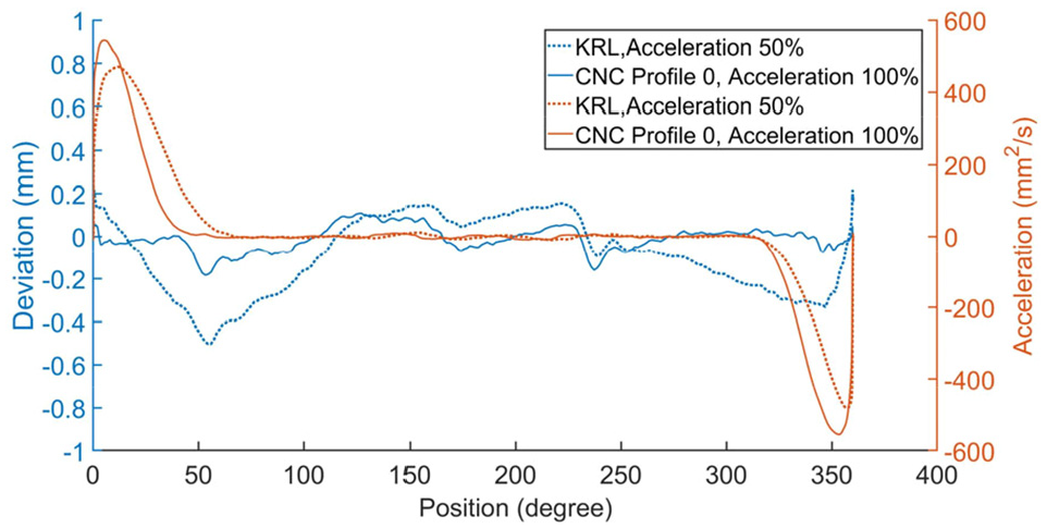
Deviation from the fitting radius and acceleration distribution along the fitting circle.

Regarding the dynamic performance of Profile 1 path, the results shows that the change in acceleration weighting has no effect on the path accuracy (Table 4). Comparing the Profile 0 path and Profile 1 path, the Profile 1 path is closer to the programmed radius and has a lower standard deviation. In addition, it has smoother movement and better control on the jerks (Figure 12), since Profile 1 determines the velocity on the programmed path while observing the specified permissible velocities, acceleration, and jerks.²⁹ As illustrated in Figure 4, the regulation of the weighting of ramp time with functions G133 and G134 can change the acceleration. Therefore, both functions are used to investigate the effect of the regulation of the ramp time on the path accuracy and acceleration distribution. In the default setting, G133 and G134 are set to 100% in Profile 1 path. Hence, G133 and G134 are set to 10%, respectively, to obtain the influence on the path. The change of G133 and G134 has almost no effect on the path accuracy (Table 4). However, the acceleration and running velocity are changed. As shown in Table 3, the maximum acceleration is increased to 171.15 mm/s² when G133 is set to 10%. However, the velocity in the steady phase remains the same as the Profile 1 path with the default setting, which results in a shorter ramp time to reach the steady phase (Figure 13(a)). When G134 is set to 10%, the maximum acceleration increases to 95.97 mm/s² (Figure 13(b)). The ramp of the acceleration profile is identical to the default setting. However, the time in the accelerating phase and braking phase increases, which promotes the velocity in the steady phase to 103.48 mm/s. These experimental analysis indicates that the effect of functions G133 and G134 on the acceleration is not exactly identical to the theoretical description (Figures 3 and 4). Because the constant feed rate is important for the machining process, it makes G133 a useful function in practical application. The time to reach the programmed feed rate can be regulated by G133.

Figure 12.

Deviation comparison between Profile 0 and Profile 1.

Figure 13.

Velocity and acceleration distribution of Profile 1: (a) velocity distribution and (b) acceleration distribution.

Conclusion

The path accuracy and acceleration distribution in circular paths under two types of control systems have been investigated. A CNC kernel, which is integrated into the robot controller and executes DIN 66025-compliant CNC programs, is beneficial for robotic machining.²⁷ Since CNC is orientated to contour, it has more functions than KR C4 to program the circular path. The experimental analysis shows that KR C4 has large deviation and obvious jerks running the circular path, which will affect the surface quality of work pieces. In addition, jerks can introduce unexpected machining force, which can damage the cutting tool. However, the CNC kernel has better performance to obtain a smooth movement under similar conditions. In addition, jerks appearing in the movement can be eliminated when the acceleration of the trapezoidal profile is selected for programming in the CNC kernel.

It indicates the key parameter is the acceleration profile. Theoretically, an acceleration profile with higher-order has low excitation of vibration. However, the improvement on the path accuracy is minor comparing step-shaped profile and trapezoidal profile. Besides, trapezoidal profile limits the motion velocity, as it takes more time for real-time calculation. Therefore, a tradeoff should be made for the robot motion planning. To simplify the programming process, an optimized acceleration profile can be adopted for the conventional robot controller according to the analysis.

Footnotes

Handling Editor: Chenhui Liang

Declaration of conflicting interests

The author(s) declared no potential conflicts of interest with respect to the research, authorship, and/or publication of this article.

Funding

The author(s) received no financial support for the research, authorship, and/or publication of this article.

ORCID iD

Kai Wu

References

Cheng

Machining dynamics: theory, applications and practices. London: Springer-Verlag, 2009.

Iglesias

Sebastián

Ares

JE.

Overview of the state of robotic machining: current situation and future potential. Procedia Eng 2015; 132: 911–917.

Wang

Industrial robotic machining: a review. Int J Adv Manuf Technol 2019; 103: 1239–1255.

Karim

Verl

Challenges and obstacles in robot-machining. In: IEEE ISR 2013, Seoul, Korea, 24–26 October 2013, pp.1–4. New York, NY: IEEE.

Devlieg

High-accuracy robotic drilling/milling of 737 inboard flaps. SAE Int J Aerosp 2011; 4: 1373–1379.

Frommknecht

Kuehnle

Effenberger

, et al. Multi-sensor measurement system for robotic drilling. Robot Comput Integr Manuf 2017; 47: 4–10.

Pandremenos

Doukas

Stavropoulos

Machining with robots: a critical review. In: 7th international conference on digital enterprise technology, Athens, Greece, September 2011.

Chen

Dong

Robot machining: recent development and future research issues. Int J Adv Manuf Technol 2013; 66: 1489–1497.

Alici

Shirinzadeh

Enhanced stiffness modeling, identification and characterization for robot manipulators. IEEE Trans Rob 2005; 21(4): 554–564.

10.

Xiong

Ding

Zhu

Stiffness-based pose optimization of an industrial robot for five-axis milling. Robot Comput Integr Manuf 2019; 55: 19–28.

11.

Sun

Liang

Fang

. Comparative study of stiffness modeling methods for a novel industrial robotic arm with hybrid open-and closed-loop kinematic chains. In: 2018 IEEE international conference on mechatronics and automation, Changchun, China, 5–8 August 2018, pp.1765–1770. New York, NY: IEEE.

12.

ABB. IRB6660 industrial robot, https://new.abb.com/products/robotics/industrial-robots/irb-6660 (n.d., accessed 12 February 2020).

13.

KUKA. KR 500 FORTEC, https://www.kuka.com/en-us/products/robotics-systems/industrial-robots/kr-500-fortec (n.d., accessed 12 February 2020).

14.

Schneider

Momeni-K

Ansaloni

, et al. Stiffness modeling of industrial robots for deformation compensation in machining. In: 2014 IEEE/RSJ international conference on intelligient robots and systems, Chicago, USA, 14–18 September 2014, pp.4464–4469. New York, NY: IEEE.

15.

Klimchik

Pashkevich

Caro

, et al. Stiffness matrix of manipulators with passive joints: computational aspects. IEEE Trans Robot 2012; 28(4): 955–958.

16.

Dumas

Caro

Garnier

, et al. Joint stiffness identification of six-revolute industrial serial robots. Robot Comput Integr Manuf 2011; 27(4): 881–888.

17.

Abele

Weigold

Rothenbücher

Modeling and identification of an industrial robot for machining applications. CIRP Ann Manuf Technol 2007; 56: 387–390.

18.

Kubela

Pochyly

Singule

. High accurate robotic machining based on absolute part measuring and on-line path compensation. In: 2019 international conference on electrical drives and power electronics, The High Tatras, Slovakia, 24–26 September 2019, pp.143–148. New York, NY: IEEE.

19.

Shu

Gharaaty

Xie

, et al. Dynamic path tracking of industrial robots with high accuracy using photogrammetry sensor. IEEE/ASME Trans Mechatron 2018; 23: 1159–1170.

20.

Shi

Zhang

, et al. An online real-time path compensation system for industrial robots based on laser tracker. Int J Adv Robot Syst 2016; 13: 1–14.

21.

Bay

KUKA.CNC-A direct approach. Auto Tech Rev 2012; 1: 54–55.

22.

MABI Robotic. MAX 100, https://www.mabi-robotic.com/robotic/robotic-arm/product.asp?IDProdukt=5 (n.d., accessed 21 April 2020).

23.

KUKA. KUKA.CNC Sinumerik, https://www.kuka.com/en-us/products/robotics-systems/software/application-software/kuka-cnc-sinumerik (n.d., accessed 21 April 2020).

24.

Möller

Schmidt

Koch

, et al. Machining of large scaled CFRP-Parts with mobile CNC-based robotic system in aerospace industry. Procedia Manuf 2017; 14: 17–29.

25.

Trendafilova

Van Brussel

Non-linear dynamics tools for the motion analysis and condition monitoring of robot joints. Mech Syst Signal Process 2001; 15: 1141–1164.

26.

Klimchik

Pashkevich

Robotic manipulators with double encoders: accuracy improvement based on advanced stiffness modeling and intelligent control. IFAC-PapersOnLine 2018; 51: 740–745.

27.

KUKA Roboter GmbH. KUKA.CNC for maximum robot performance in machining processes, https://pdf.directindustry.com/pdf/kuka-ag/kukacnc-maximum-robot-performance-machining-processes/17587-435805.html. (2011).

28.

KUKA Roboter GmbH. KUKA System Software 8.2 operating and programming instructions for system integrators. Augsburg, Germany: KUKA Roboter GmbH, 2011.

29.

Industrielle Steuerungstechnik GmbH. Programming manual. Stuttgart: Industrielle Steuerungstechnik GmbH, 2010.

30.

Brueninghaus

Johnen

, et al. Applicability of stereo high speed camera systems for robot dynamics analysis. In: 2015 international conference on control, automation and robotics, Singapore, 20–22 May 2015, pp.44–48. New York, NY: IEEE.

31.

Krewet

Bickendorf

, et al. Dynamic performance of industrial robot with CNC controller. Int J Adv Manuf Technol 2017; 90: 2389–2395.

32.

GOM mbH. PONTOS user manual – software. Braunschweig, Germany: GOM mbH 2008.

33.

Janabi-Sharifi

Hayward