
Abstract
Resilient teams overcome sudden, dynamic changes by enacting rapid, adaptive responses that maintain system effectiveness. We analyzed two experiments on human-autonomy teams (HATs) operating a simulated remotely piloted aircraft system (RPAS) and correlated dynamical measures of resilience with measures of team performance. Across both experiments, HATs experienced automation and autonomy failures, using a Wizard of Oz paradigm. Team performance was measured in multiple ways, using a mission-level performance score, a target processing efficiency score, a failure overcome score, and a ground truth resilience score. Novel dynamical systems metrics of resilience measured the timing of system reorganization in response to failures across RPAS layers, including vehicle, controls, communications layers, and the system overall. Time to achieve extreme values of reorganization and novelty of reorganization were consistently correlated with target processing efficiency and ground truth resilience across both studies. Correlations with mission-level performance and the overcome score were apparent but less consistent. Across both studies, teams displayed greater system reorganization during failures compared to routine task conditions. The second experiment revealed differential effects of team training focused on coordination coaching and trust calibration. These results inform the measurement and training of resilience in HATs using objective, real-time resilience analysis.
Introduction
Effective teams efficiently coordinate heterogeneous and shared resources to accomplish shared and valued goals (Salas et al., 2008). In this context, a resilient team responds to undesirable conditions and challenges, such as system failures, by rapidly reorganizing its resources to maintain high levels of team performance (Alliger et al., 2015; Morgan et al., 2017). It is theorized that resilient teams accomplish this by rapidly recognizing, designing, and implementing changes to ward off novel impediments to team effectiveness outside their current areas of capable performance (Hoffman & Hancock, 2017). Lack of team resilience is exemplified in the 1996 Mount Everest climbing disaster, in which eight climbers died while climbing Mount Everest. A lack of team learning—including ill-defined purpose, vague leadership, and poor sensemaking—were key contributors to this disaster, but this disaster was at least partially attributable to a breakdown of team coordination (Kayes, 2004). Lack of resilience and coordination was also observed in the delayed response to Hurricane Katrina (Leonard & Howitt, 2006), in which a more rapid system reorganization may have sped up relief and the subsequent recovery of those impacted by the storm surge (Colten et al., 2008). In contrast, rapid reorganization of system resources has been associated with timely and effective responses (e.g., military-civilian evacuation efforts following 9/11; Boin & Bynander, 2015). In line with Hoffman and Hancock (2017), we propose that more resilient teams exhibit faster detection of impending catastrophes, implementation of required changes (i.e., reorganization behavior), and are thus able to recover from novel threats more rapidly.
Emergency response in aviation and other power system failures are long-standing concerns in resilience research (e.g., Woods et al., 1988). We build on this research by applying an objective, data-driven approach to measuring team resilience with the potential for real-time analysis that can provide training, feedback, and identify critical sources of system reorganization underlying resilience. We focus on human-autonomy teaming (HAT), which is defined as teams in which humans work with technological agents that are intelligent and autonomous enough to be considered a teammate (McNeese et al., 2018). The study of HATs increasingly applies to safety-critical domains, including urban search and rescue (Krujiff et al., 2014), uninhabited aerial systems (McNeese et al., 2018), cyberspace operations (Tambe et al., 1999), and self-driving autonomous vehicles (Campbell et al., 2010). By enabling flexible, adaptive, and rapid team responses (Hoffman & Hancock, 2017; Hollnagel et al., 2007), a resilient HAT would be better equipped to rapidly overcome potential pitfalls associated with unpredictable challenges, such as automation and autonomy failures, cyberattacks, communication link failures, and system power outages. Many of these common pitfalls in HATs are associated with brittleness, lack of transparency, miscalibrated trust, and a lack of shared awareness (Shively et al., 2017). For example, although a human working with an autonomous agent may lack shared situation awareness with the agent, a resilient HAT would be more likely to overcome an error resulting from this lack of shared awareness by quickly reorganizing how it coordinates across system layers. These potential pitfalls associated with HATs make these types of teams suitable for studying resilience.
In this paper, we describe a method for measuring team resilience in response to technological system failures (i.e., automation and autonomy failures), system power-downs, communication outages, and cyberattacks using the concept of system reorganization (Stevens et al., 2016). Reorganization refers to how a team dynamically alters its patterns of interaction, including communication and coordination, across human and technological system layers to adapt and overcome system failures. By measuring reorganization in response to failure perturbations, we aim to create objective metrics for measuring resilience that correlate with established measures of team performance. In addition, by correlating resilience metrics with team performance, we hope to better understand the nature of resilience, in which faster reorganization is hypothesized to correlate with increased team effectiveness. Thus, the primary focus of this paper is to present novel dynamical systems metrics of team resilience and validate them across a series of HAT experiments.
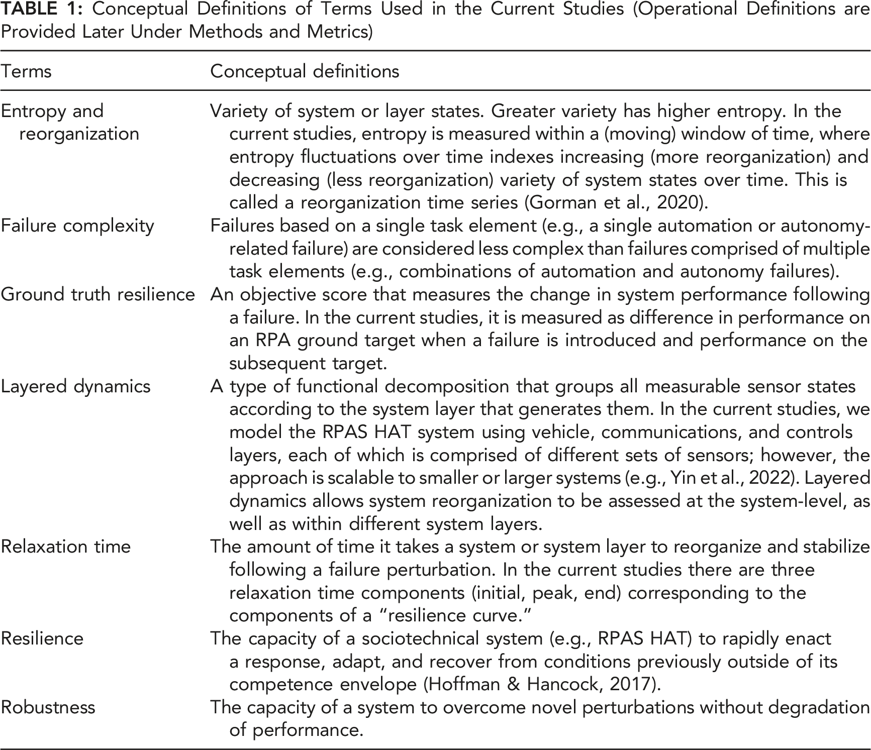
Conceptual Definitions of Terms Used in the Current Studies (Operational Definitions are Provided Later Under Methods and Metrics)
Systems Approach
Resilience engineering is relevant to the training and development of effective teams across a variety of settings. Resilience engineering emphasizes how sociotechnical systems of varying sizes, from teams to large organizations, are expected to encounter disturbances, errors, and perturbations, and how these systems flex and adapt to maintain peak performance (Hollnagel et al., 2007). In this light, the development of bottom-up, data-driven approaches to quantify and visualize team resilience that have the potential for real-time resilience analysis are a critical need. We will measure team resilience using metrics based in dynamical systems theory, with the goal of integrating real-time dynamical methods with concepts of team resilience in human factors and resilience engineering.
In resilience engineering, resilience is defined as the “systemic capacity to change [i.e., reorganize] because of circumstances that push the system beyond the [current] boundaries of its competence envelope” (Hoffman & Hancock, 2017, pp. 565–566). The RPAS synthetic task environment is appropriate for analyzing team resilience because it allows for the controlled introduction of different types of technology failures, referred to as perturbations, which are external forces that require a system to reorganize to remain in or find a new stable state (Gorman, Cooke, & Amazeen, 2010). In terms of resilience engineering, perturbations force teams to operate beyond the boundaries of their initial training. We analyze team resilience in the context of failure perturbations that provide a test of a team’s ability to adapt to and overcome different types of HAT failures.
Because teams in dynamic environments continuously self-organize new arrangements of parts as they adapt to the changing environment, we view teams as complex adaptive systems (Elliott & Kiel, 2022; McGrath et al., 2000). Therefore, our measures focus on the coordinated behavior that emerges from individual-level interactions, as opposed to the individual-level actions themselves (Amazeen & Amazeen, 2017). When examining the coordinated behavior of human and technological components of a system, resilience can be viewed as the ability for components to mutually adapt when encountering unexpected perturbations and quickly recover to maintain stable and effective system performance. Thus, resilience involves maintaining system performance across human and technological components to maintain a stable trajectory directed toward accomplishing team goals (“teleological variation,” Gorman et al., 2019; Thorén, 2014). The time course of a system to re-stabilize or stabilize in a new state following a perturbation is called relaxation time (Trotsky et al., 2012), which is an index of the system’s ability to enact a response, adapt, and recover following a perturbation (Abraham & Shaw, 1992; Mermin, 1970). In the current studies, we use the concept of relaxation time to measure how long it takes a HAT to reorganize following autonomy, automation, and other system failures to identify the reorganization profiles across system layers that correspond to different types of failure perturbations.
The Current Studies
Our relaxation time metrics of resilience are based on a nonlinear prediction algorithm (Kantz & Schreiber, 1997) and layered dynamics (Gorman et al., 2019). We used these algorithms to measure (a) how quickly a team reorganizes system behavior in response to a perturbation, (b) the novelty of the reorganization, and (c) which system layers (operator communications, controls, vehicle, system overall) reorganize in response to failure perturbations. To examine the association between these resilience metrics and maintaining team effectiveness, we correlated them with objective team performance measures, including a team performance outcome score, a processing efficiency score, and a binary score of whether the team overcame the failure. We also correlated the relaxation time resilience metrics with a ground truth resilience score, which measures the change in the efficiency of taking photos of ground targets (the primary goal of RPAS missions) during and immediately following a failure perturbation. Thus, the team performance metrics and ground truth resilience score provided a test of criterion validity for the relaxation time resilience metrics. The purpose of testing our resilience metrics across different RPAS HAT experiments was to understand how these measures react to automation and autonomy failure perturbations (Experiment 1) and failure perturbations of increasing complexity (Experiment 2), as well as their sensitivity to HAT training manipulations, which were hypothesized to differently impact response to either automation or autonomy failures, as described in the Experiment 2 Methods section. The next section outlines the general method used in both experiments; the details of the participants and procedures of each experiment are separately provided in later sections. Study hypotheses are heavily informed by the design of the dynamical systems resilience metrics; hence, specific hypotheses are presented after the General Method, Measures section.
General Method
Overview
Results are reported from two experiments conducted at the Cognitive Engineering Research Institute (CERI) at Arizona State University. The data were collected in the Cognitive Engineering Research on Team Tasks RPAS Synthetic Task Environment (CERTT-RPAS-STE), which simulates teamwork components of RPAS operations and allows for system-level evaluations of these components. The two experiments use the CERTT-RPAS-STE but differ with respect to between- and within-subjects manipulations.
Materials
The CERTT-RPAS-STE consists of seven hardware consoles (three for task roles, four for experimenters) in which participants and experimenters use a chat interface to communicate (Grimm et al., 2018; McNeese et al., 2018). The task consists of three team-member roles: (1) a navigator who creates the flight plan and sends waypoint restrictions (altitude, airspeed, waypoint name and type, effective radius) to the pilot and photographer; (2) a pilot who monitors and controls vehicle altitude, heading, and airspeed based on the flight plan, and maintains fuel, gears, and flaps settings; additionally, the pilot negotiates with the photographer to achieve required altitude and airspeed to enable successful photographs of target waypoints; and (3) a photographer who controls camera type and settings, takes target photos, and communicates feedback of the target photo results to the navigator and pilot. Each team member has three screens, including a screen that displays role-specific information, a screen that presents RPA status (e.g., current target; speed; altitude; distance to target), and a chat interface screen. The goal of the team is to fly the RPA through a series of target waypoints (11–20 per mission) to take reconnaissance photos while meeting waypoint restrictions (i.e., acceptable speed/altitude) and to minimize warnings and alarms during a series of 40-min missions.
This research sought to understand resilience in HATs under degraded conditions, which is a term used to specifically refer to automation, autonomy, and malicious attack failures (Cooke et al., 2020). In the current studies, the navigator and photographer were informed that the pilot was an autonomous agent, although the autonomous agent was actually a trained experimenter. Known as the Wizard of Oz paradigm (WoZ; Kelley, 1983), this technique was used to introduce autonomy failures in a controlled manner rather than programming an autonomous agent that failed in controlled ways. Other than introducing autonomy failures, the WoZ pilot emulated the behavior of an actual autonomous agent pilot, known as the synthetic teammate (Ball et al., 2010). The synthetic teammate was developed using Adaptive Control of Thought-Rationale (ACT-R; Anderson et al., 1997) and interacts with human teammates through text chat and is responsible for all taskwork aspects of the pilot role. Prior work with the synthetic teammate revealed limitations of the agent’s communication and coordination capabilities (McNeese et al., 2018; Scalia et al., 2022), which were replicated using the WoZ paradigm in the current studies. Therefore, participants (navigator and photographer) were given cheat sheets to assist in effective communication with the WoZ pilot.
Measures
Performance Metrics
We measured team effectiveness using three performance scores. Team Performance was a mission-level outcome score, that emphasized the overall ability to successfully photograph targets while accounting for other mission parameters, including time spent in warning/alarm states, number of good photographs, missed targets, and fuel and battery consumption. Teams started each mission with a score of 1,000, and points were deducted based on those parameters. Overcome measured how many failures teams successfully overcame, defined as the team successfully photographing the target impacted by the failure. If the team overcame the failure, they received a 1, and if they failed to overcome the failure, they received a 0. Finally, Target Processing Efficiency (TPE) measured performance at the target level based on how much time the team spent in the effective target radius to take a photo (shorter times are more efficient). TPE was negatively scored, such that higher scores corresponded to greater efficiency (range = 0–1000). The closer the score to 1,000, the better the TPE; however, there was no a priori range regarded as optimally efficient TPE. Team performance and overcome are outcome-based measures, whereas TPE is a process-based measure, as it deducts points for inefficient team processing while in the target radius. Overcome was scored 1 if the team successfully obtained a good photo of the failure target and 0 if not; all other performance scores were generated automatically by the task software.
Ground Truth Resilience Score
The ground truth resilience score (GTRS) is a process-based measure of team resilience computed from TPE scores. GTRS measures the performance difference between TPE on the failure target and TPE on the subsequent target. Conceptually, GTRS measures both how much a team is initially impacted by a failure and how well a team recovers following the failure. This score is calculated as the difference between TPE on the failure target and TPE on the following (non-failure) target (Equation (1)).
Although GTRS was intended to measure behavioral resilience, it does not directly measure how this occurs. For example, if TPE is greatly reduced by a failure, but TPE on the subsequent target returns to a high level, then GTRS would be large, which would fit the concept of resilience as recovery (Woods, 2015). In this case, we should observe a negative correlation between larger GTRS and shorter relaxation times. On the other hand, if a team reorganizes so quickly (shorter relaxation time) that TPE on the failure target remains high, and TPE on the subsequent target also remains high, then GTRS would be small, and this would fit the concept of resilience as robustness (Woods, 2015). It is also possible for low-performing teams, who were poor on the failure target and the subsequent target (i.e., TPE small on both occasions), to obtain a small GTRS. In these latter cases, we should observe a positive correlation between smaller GTRS and shorter relaxation times.
Dynamical Systems Resilience Metrics
Layered Dynamics
We analyzed four layers of RPAS coordination that represent HAT reorganization (Gorman et al., 2019). System layers included (1) communication layer – message sending and receiving among team members through the chat system (i.e., pilot → navigator; navigator → pilot and photographer; etc.); (2) vehicle layer – actions and states of the vehicle (i.e., changes in speed; altitude; fuel; heading; etc.); (3) controls layer – the controls used to interface with the vehicle and other teammates (i.e., changes in pilot’s vehicle controls; photographer’s camera controls; navigator’s route planning controls; etc.); and (4) system layer – overall system state across all layers.
A vector of binary symbols represents the states of all system components, within each layer and the system overall, as a time series (1 Hz). The sensors within the layers—Communication = 9, Vehicle = 9, Controls = 21—comprise an overall RPAS state vector (Figure 1). This overall RPAS vector (i.e., the “system layer”) is thus a 39-component vector. For continuous variables, states were determined by mapping the continuous dynamics of components onto a numeric alphabet for symbolic time series modeling (Nicolis & Prigogine, 1989) that preserves the dynamics (e.g., vehicle speed can be represented using four states/symbols: speeding up; slowing down; constant speed; alarm state; Gorman et al., 2019). The purpose of using symbolic dynamics is that by defining the symbols as mutually exclusive and collectively exhaustive symbol sets, we can sum across any collection or sensor states at 1 Hz (e.g., just the vehicle layer vs. the system overall) to efficiently obtain set intersections representing unique layer and system states. This method allows for the efficient computation of changing system and layer states on a second-by-second basis (Gorman et al., 2019). Input component signals for the Vehicle, Controls, and Communication layers. Non-underlined component in the Vehicle layer provide redundant information and were not used. Figure adapted from Gorman et al. (2019).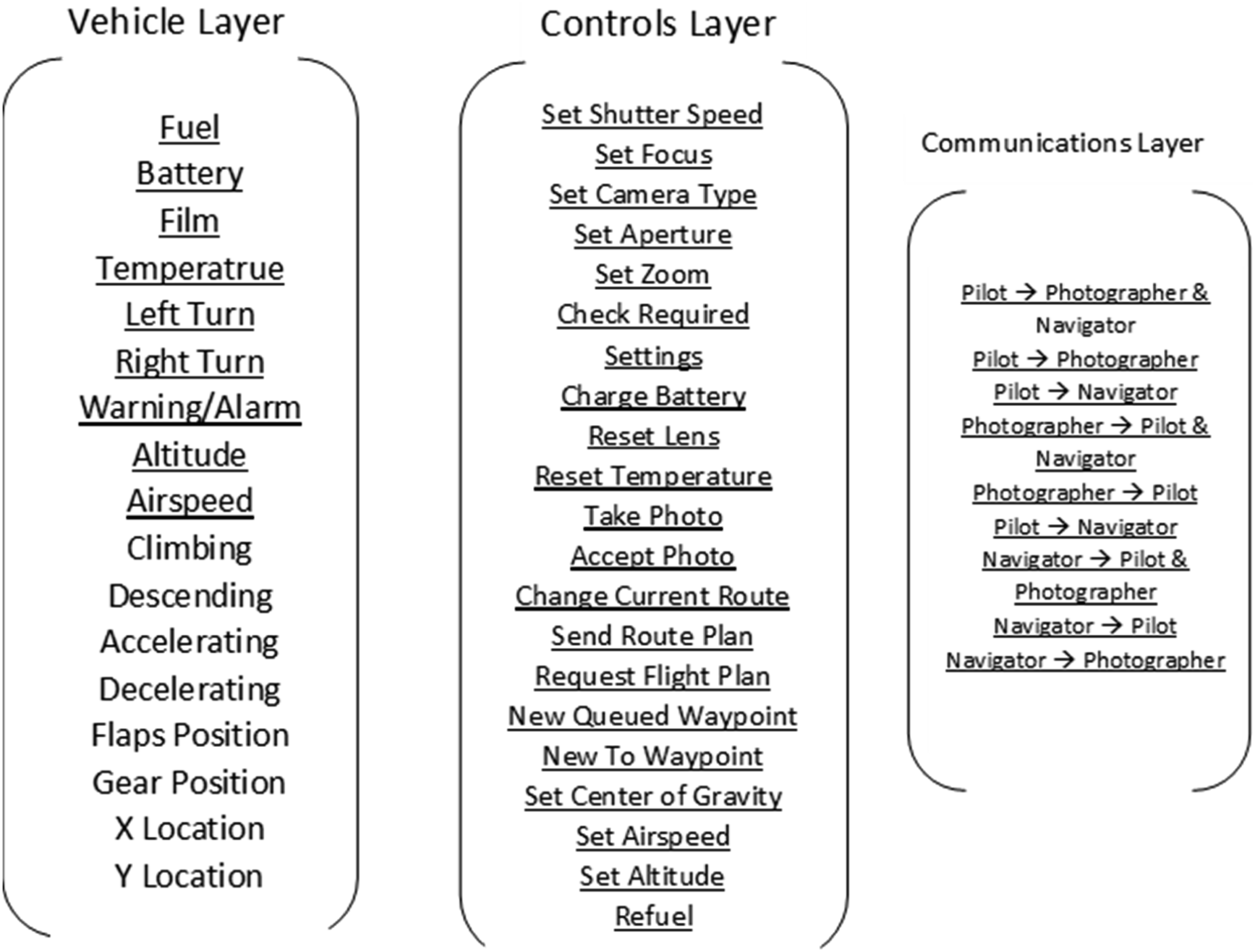
Although the symbolic alphabet is numeric to allow for summation, we do not assume any ordinal relations (e.g., greater than) among the symbols. As illustrated in Figure 2, it does not matter what the symbols are except that the symbolic time series for each component sensor must be mutually exclusive with all other components, such that summing across component states yields a unique intersection (∩) for every unique system state. In Figure 2, the numeric symbols are binary numbers, with addition through horizontal concatenation. The purpose of using binary numbers is that it facilitates the scalable expansion of the mutually exclusive and exhaustive symbol sets if needed (e.g., if we needed to add another component to the system). Example illustrating symbolic time series using binary symbols for component states (qi = component i state; 000 = off state) and team state (Q’; component intersections) obtained by summing across (binary addition) component states at each time point (sample). For illustration, this example uses two on/off state for each component; however, the method is generalizable to higher order component states as in the current studies.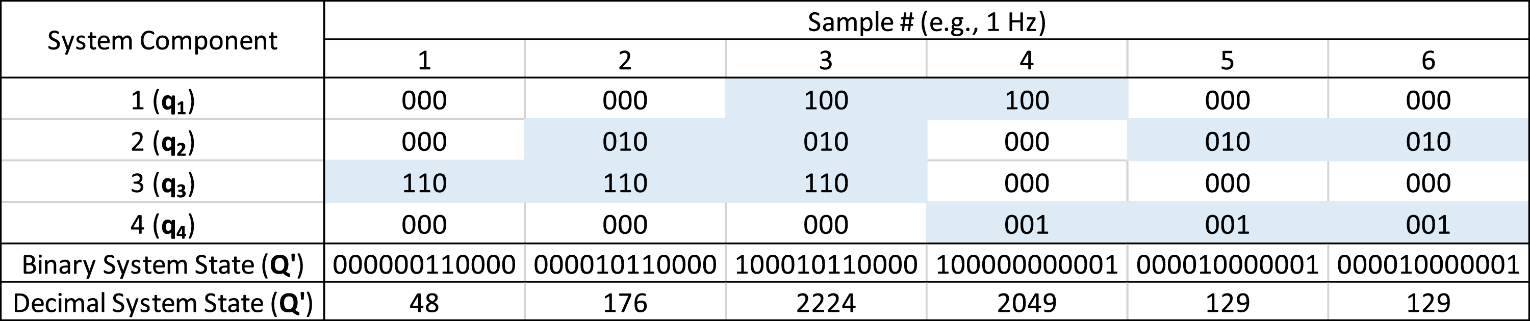
Reorganization
The following section describes the calculation of reorganization time series using layered dynamics. All data management and analytic procedures were the same across both experiments.
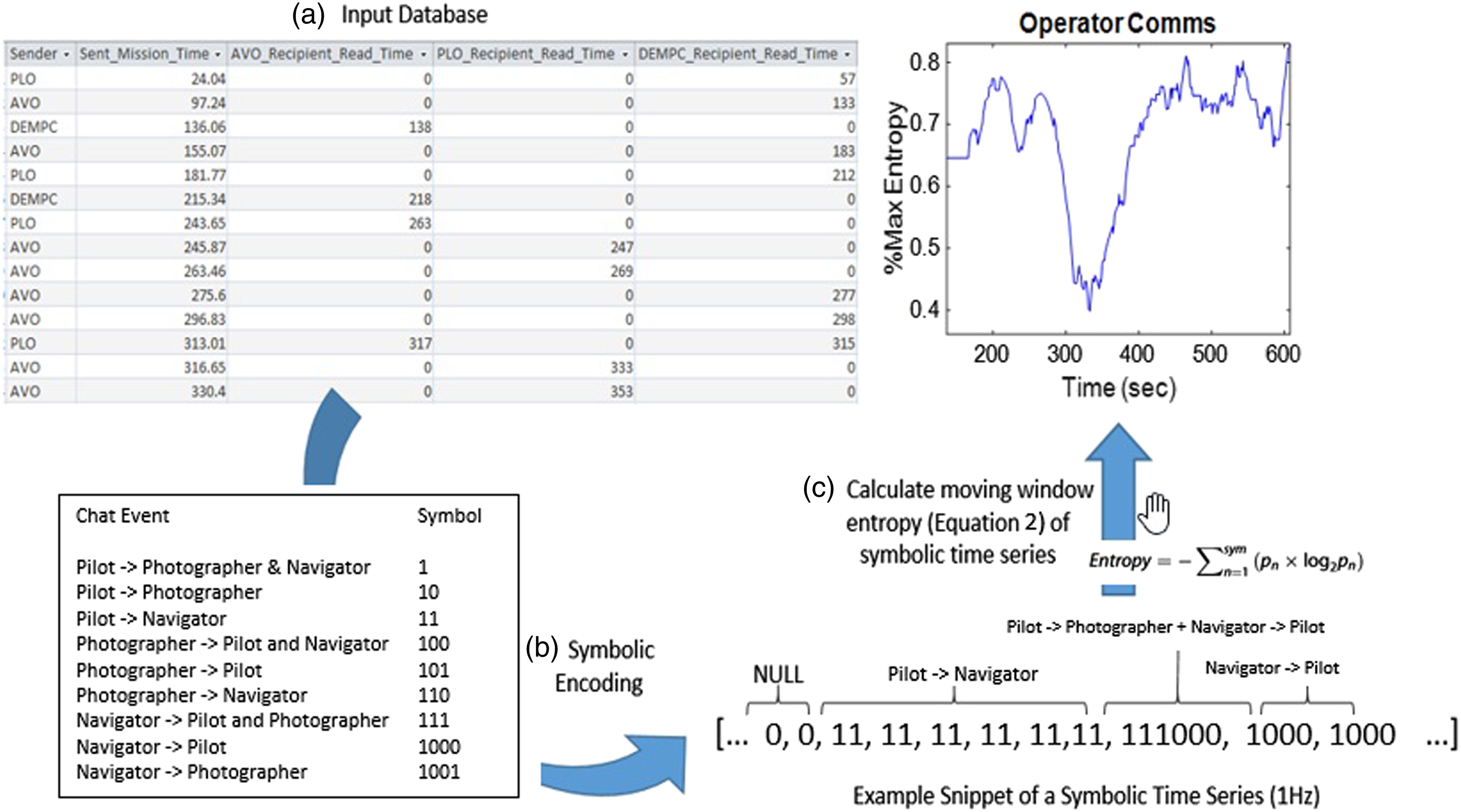
Entropy (Equation (2)) is a measure of the variety of system states within a window of time (Ashby, 1957), and moving window entropy is a continuous measure of the changing variety (“reorganization”) of system states over time (Gorman et al., 2020; Stevens et al., 2016). In equation (2), pn is the relative frequency of any of the n states in the window multiplied by log2 Illustration of moving window entropy calculation: (a) input database of text chat events generated by the task software (only time sent and read were used; content was not analyzed); (b) symbolic encoding represents each possible “From-To” chat event as a binary symbol; (c) moving window entropy calculated from (1 Hz) symbolic time series of chat events (higher entropy = more reorganization/variety). Figure adapted from Gorman et al. (2019).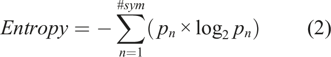
The purpose of encoding sensor data using mutually exclusive states is that every unique intersection of sensor states (e.g., intersecting a Vehicle state with a Communication state) defines some new state. The possible combinations of sensor states for measuring system state (or layer state, if desired) can be enormous. A conservative estimate of the number of the possible system states in the current studies if each of the 38 sensors take on at most two states would be 238 = 274,877,906,944 unique system states. It is unlikely that all portions of this state space will ever be visited by the system: Some portions of the state space are likely to be visited more frequently than others (cf. attractors), whereas some portions of the state space may be inaccessible to the system (cf. repellors). Note, however, that the purpose of the present studies is not to enumerate specific states and attractors of the system; we leave that for future research, but to use layered dynamics models to develop generalizable real-time resilience metrics.
Reorganization Novelty
We used Kantz and Schreiber’s (1997) nonlinear prediction algorithm to quantify reorganization novelty in terms of deviations (root mean square error; RMSE) of the observed reorganization time series from a predicted behavior reorganization time series. RMSE represents how different the current reorganization trajectory is from the predicted trajectory based on prior reorganization behavior (Figure 3).
For a reorganization (entropy) time series, select the current value,
For the current studies, we set ε = 3 and Δn = 20s, which have been shown to be effective for detecting novel system reorganization during perturbations in medical and submarine domains (Gorman et al., 2020; Grimm et al., 2017). RMSE time series were generated for each RPAS mission using the same moving window procedure described previously for entropy (Figure 4). Depiction of the RMSE calculation. Larger deviations between observed (“Raw”) and predicted (“Expected”) yield larger RMSE values indicating greater reorganization novelty.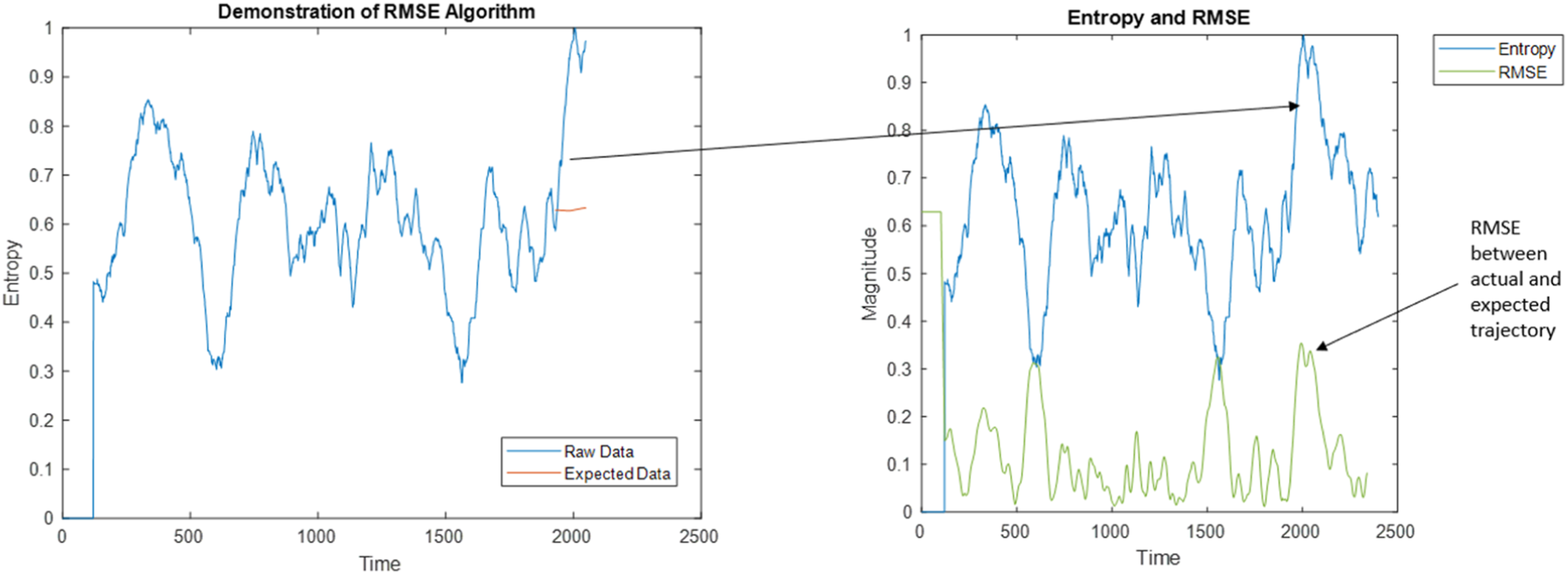
Relaxation Time
Dynamical systems approaches for studying team adaptation typically involve introducing perturbations to determine how the team responds through verbal communication reorganization (e.g., Gorman et al., 2020; Grimm et al., 2017). Using this approach, relaxation time is the time it takes for a team to adapt and recover by reorganizing following a perturbation. If this happens quickly, then the team’s relaxation time is shorter. We define relaxation time as being made up of three components in line with the theoretical approach of Hoffman and Hancock (2017). Whereas relaxation time and resilience are often thought of as a singular time to rebound (Woods, 2015), we break it down into three functionally meaningful parts (Initial, Peak, End). In the current studies, we measure these relaxation time components across the sociotechnical system—across communication, vehicle, controls layers, and the system as a whole—in response to failure perturbations.
The first relaxation time component, Initial, is how long (in sec.) it takes a team’s reorganization time series to exceed a 99% confidence interval (CI) following perturbation onset (described in detail later). The Initial measure operationalizes how quickly the team enacts a reorganization in response to a failure and represents the enaction component of resilience. The second component, Peak, is how long (in sec.) it takes reorganization to reach its most extreme value following perturbation onset. The Peak measure operationalizes how quickly the team reaches its maximum point of reorganization and represents the adaptation component of resilience. To parallel Hoffman and Hancock (2017), Initial measures the time to recognize the need for and enact a change, whereas Peak measures the time to implement the change (i.e., adaptation).
The third component, End, measures how long it takes for a team to return to a non-significant level of reorganization following enaction and adaptation. The End measure is defined as the last time point (in sec.) at which the reorganization time series is operating at statistically extreme levels (exceeds 99% CI) following a failure perturbation. This third metric closes the “resilience curve” comprising enaction, adaptation, and recovery (Figure 5), with recovery defined as a return to nominal levels of reorganization. As shown in Figure 5, all relaxation time component measures are calculated relative to a 99% CI computed over the reorganization time series from failure perturbation onset to perturbation offset. The purpose of using the distribution of observations within a failure’s duration was to ensure that each of the three relaxation time components (Initial, Peak, End) could be measured for every failure perturbation. Resilience measurement components that complete a “resilience curve.” The black trace represents moving window entropy over time, and the red line represents the 99% confidence interval (CI) used to measure Initial, Peak, and End relaxation time components. This figure illustrates resilience metrics for an entropy reorganization time series; however, the process is identical for measuring resilience for an RMSE reorganization novelty time series.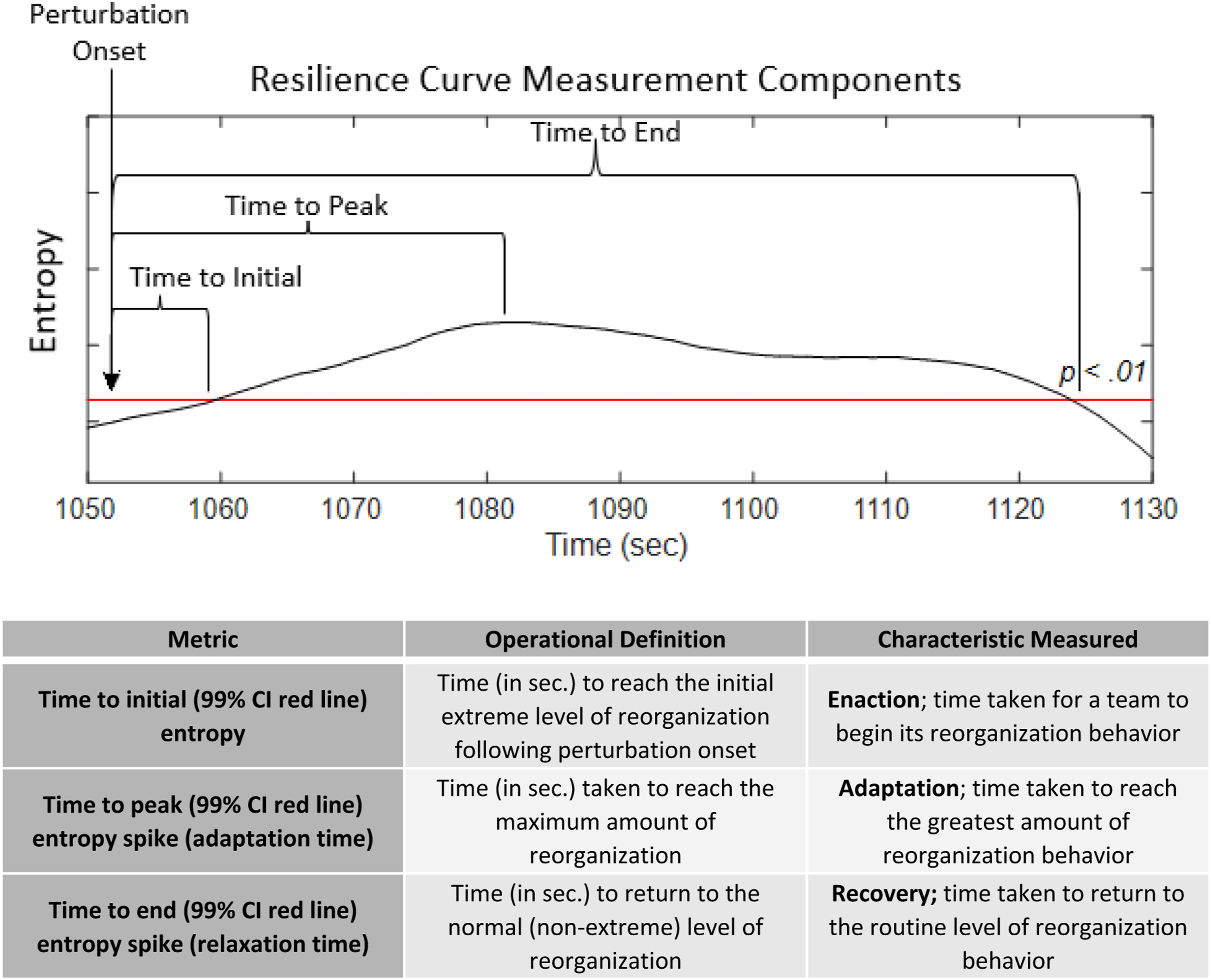
Because the sampling rate was 1 Hz, the number of possible reorganization observations during a perturbation simply corresponds to the duration (in sec.) of the perturbation. Perturbation failure length ranged from 300–420 seconds in Experiment 1 (Cooke et al., 2020) and 300–600 seconds in Experiment 2 (Johnson et al., 2020). Relaxation times were always measured relative to the onset of perturbation, such that more rapidly closing the resilience curve (Figure 5) would result in relaxation times shorter than the full perturbation duration.
Study Hypotheses
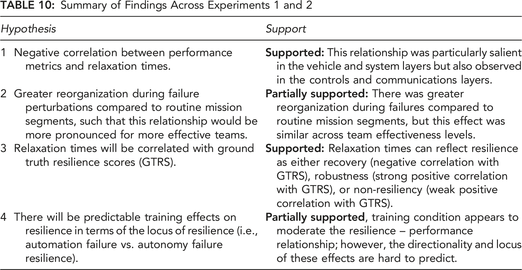
Our first hypothesis examined how relaxation time metrics relate to maintaining team effectiveness. We hypothesized that shorter relaxation times, which indicate faster enaction, adaptation, and recovery, should be associated with higher team performance. • Hypothesis 1: Shorter relaxation times (greater adaptive ability/recovery) will be correlated with greater team effectiveness (higher performance scores) across both experiments.
Our second hypothesis was that RPAS HATs should exhibit significantly greater system reorganization during failure perturbations compared to routine mission conditions containing no failures. This hypothesis is akin to the law of requisite variety (Ashby, 1957), which states that for a system to maintain effectiveness, the controller (“team”) must be able to produce sufficient coordination variety (variety = number of states) to match or exceed the variety demanded by the environment. We further hypothesized that this increase in reorganization behavior would be larger for more effective teams. • Hypothesis 2a: Teams will exhibit greater reorganization behavior during failure perturbations compared to routine mission segments. • Hypothesis 2b: This effect will be larger for higher-performing teams.
We examined criterion validity by correlating our resilience metrics with a ground truth resilience score, which measured the impact and subsequent recovery of performance following a failure perturbation. As described earlier, whether the correlation between our resilience metrics and ground truth resilience was negative or positive indicates either the classic form of resilience as recovery or resilience as robustness to perturbation (Woods, 2015). Therefore, our hypothesis with respect to ground truth resilience was non-directional. • Hypothesis 3: Relaxation times will be correlated with ground truth resilience, with the direction of correlation indicating the nature of resilience (i.e., recovery vs. robustness).
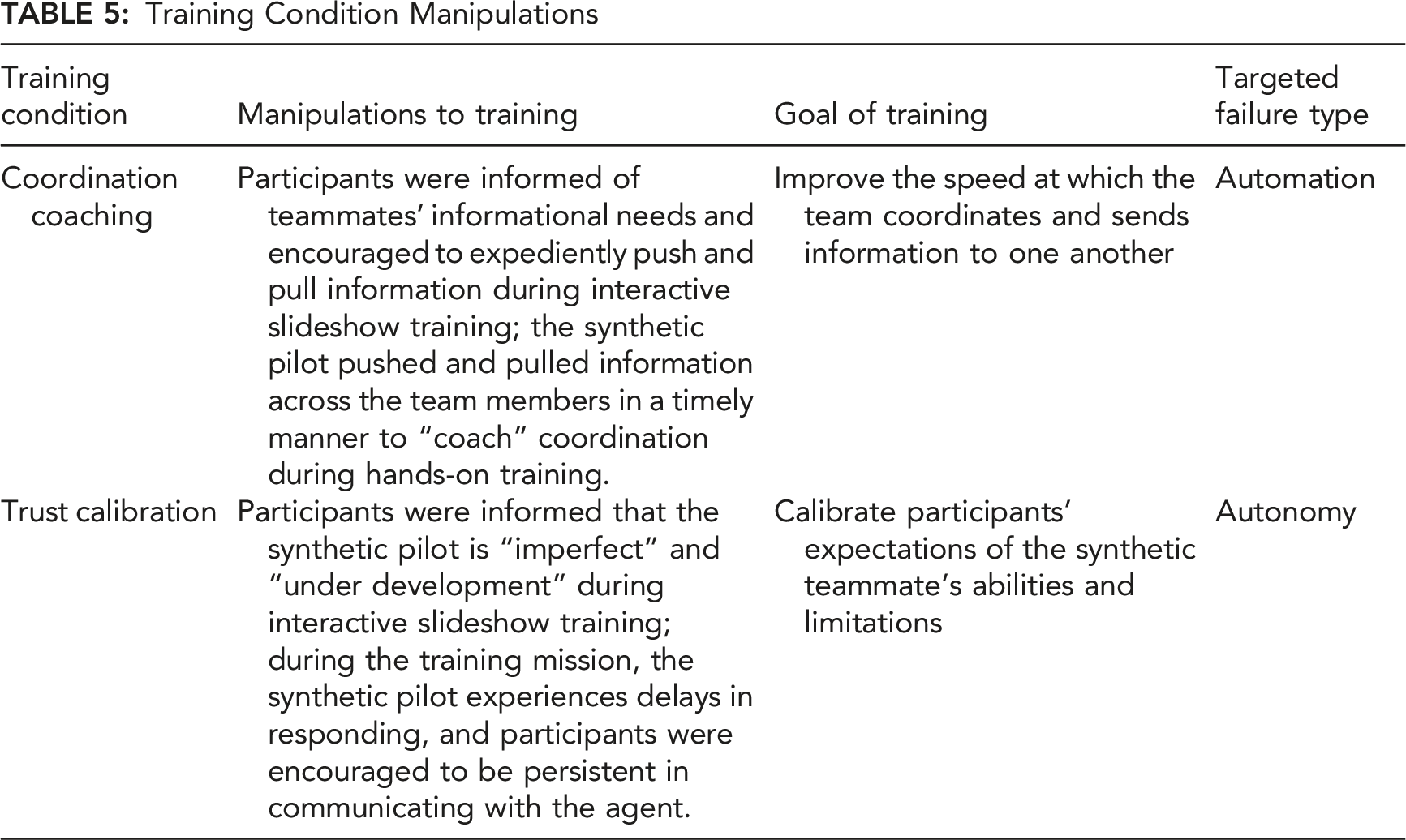
In Experiment 2, teams received different types of training designed to help them overcome either automation failures (“Coordination Coaching”) or autonomy failures (“Trust Calibration”), with a third group receiving no special training (“Control”). Because coordination coaching was intended to help teams overcome automation failures, and Trust Calibration was intended to help teams overcome autonomy failures (Johnson et al., 2020), we hypothesized that our resilience metrics would reflect this difference. Specifically, we predicted that relaxation time-performance/GTRS correlations would be stronger for automation failures for Coordination Coaching teams, whereas these correlations would be stronger for autonomy failures for Trust Calibration teams. These two training conditions, Trust Calibration and Coordination Coaching, are described in detail in the Experiment 2 Methods section. • Hypothesis 4: Teams receiving coordination coaching will display greater resilience in the form of stronger resilience correlations for automation failures, whereas teams receiving trust calibration training will display stronger resilience correlations for autonomy failures.
Hypotheses 1–3 (but not 4) were tested in both experiments. Therefore, in the following results sections we refer to each hypothesis according to its experiment and hypothesis number. For example, Experient 1, Hypothesis 1 is labeled E1.H1, Experient 2, Hypothesis 1 is labeled E2.H1, etc.
Experiment 1
Participants
Forty-four participants (22 teams) between 18 to 36 years of age (M = 23.0, SD = 3.90) were recruited from Arizona State University and surrounding areas. The gender distribution was 21 males and 23 females. Participants were required to have normal or corrected-to-normal vision and fluency in English. All participants were compensated $10 per hour. The experiment was approved by the Cognitive Engineering Research Institute Institutional Review Board.
Procedure
Experiment 1 took place across two sessions, with a one- to two-week interval between sessions. A trained experimenter was placed in the pilot role and performed as the autonomous agent in a WoZ paradigm (Kelley, 1983) using a script to mimic actions and communications consistent with the synthetic teammate. Participants were randomly assigned to either navigator or photographer and were instructed that they were working with a synthetic teammate. The experimenter in the synthetic teammate role was in a separate room, and the participants were located together in another room and were separated by a partition. Each participant individually received 30 min of PowerPoint training on the task and their roles. Subsequently, they performed a 30 min hands-on training mission as a team, during which other experimenters used a checklist to ensure that the navigator and photographer were sufficiently trained in their roles.
Procedure for Experiment 1
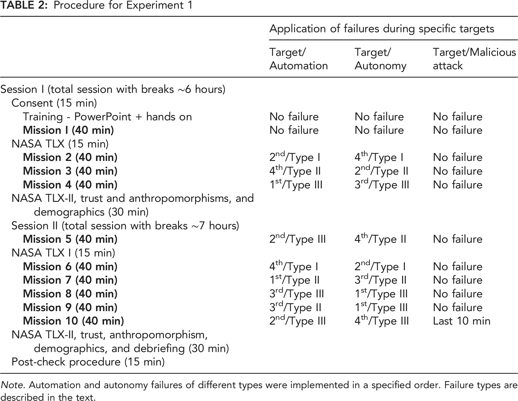
Note. Automation and autonomy failures of different types were implemented in a specified order. Failure types are described in the text.
Failure Types
This section describes the three types of automation and autonomy failures. Because the malicious cyberattack occurred only once, it was not included in the inferential statistical analysis of Experiment 1. However, the malicious attack failure was examined in Experiment 2, due to its importance for examining failure complexity.
Automation Failures
The Type I Automation Failure affected the photographer for a total duration of 300 sec. This failure prevented the photographer from viewing current and next target waypoint information, remaining time, distance to the current target, bearing, and course deviation to target, such that the photographer had to obtain that information by communicating with other team members. The Type II Automation Failure affected the pilot for a total duration of 420 sec. This failure prevented the pilot from viewing current altitude and airspeed settings and from entering new altitude and airspeed information, such that the pilot had to obtain that information by communicating with other team members. The Type III Automation failure also affected the pilot for a duration of 420 sec. This failure was more intense than the Type II automation failure. In addition, the pilot was unable to see the remaining time, distance, and bearing to the current target waypoint, such that the pilot had to communicate with other team members to obtain accurate target information. Figure 6 displays an example of a Type II automation failure. Example of a Type II automation failure. The left image displays the pilot’s screen during normal (routine) conditions. The right image displays the failures that occurred during the Type II automation failure: The pilot cannot see Altitude and Airspeed and must obtain this information from other team members.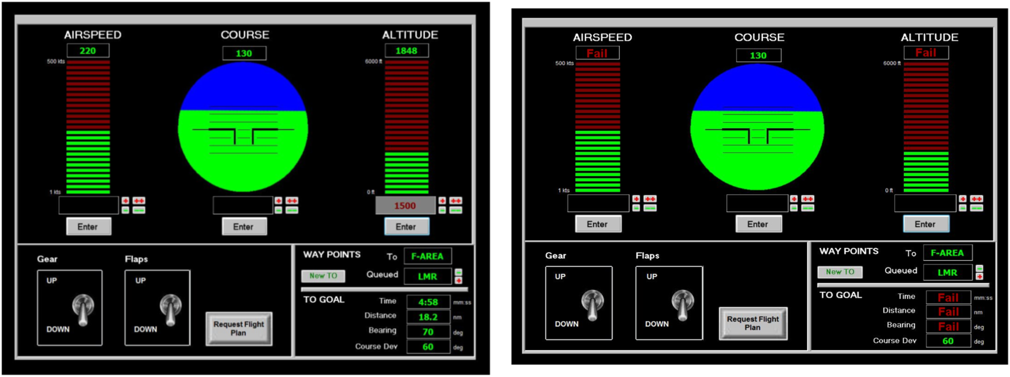
Autonomy Failures
The experiment included three types of autonomy failures in which the synthetic teammate pilot failed, each lasting 420 seconds. The Type I Autonomy Failure was a comprehension failure in which a human team member provided information to the synthetic agent, but the agent repeatedly requested the same information due to its inability to comprehend. To overcome this failure, the human team member had to notice the synthetic pilot’s incorrect behavior and re-send the correct target waypoint information (i.e., required altitude and airspeed; Cooke et al., 2020). The Type II Autonomy Failure was an anticipation failure in which the synthetic agent did not give the photographer sufficient time to take a good photo and prematurely changed course to the next target. To overcome this failure, the photographer or navigator must notice this failure and instruct the pilot to go back to the target waypoint. The Type III Autonomy Failure was also a comprehension failure in which the synthetic agent failed to understand a message due to its limited communication abilities and misinterpreted target information (altitude, airspeed) from the navigator and photographer. To overcome this failure, the photographer had to repeat the correct information until the pilot correctly adjusted the necessary settings.
Data Analysis Overview
To classify reorganization or novelty values as exceeding the critical threshold, we focused on the distribution of observations within the timespan of a failure, and identified reorganization observations that exceeded the 99% CI of the observations within the timespan of that failure, corresponding to a .01 alpha level (Cohen et al., 2013). From these extreme values, we calculated the relaxation time component metrics (i.e., Initial, Peak, and End) for each failure perturbation. To test H1 (shorter relaxation times are correlated with greater performance), H3 (relaxation times are correlated with GTRS), and H4 (training effects will be present), we correlated each relaxation time component for each system layer (Vehicle, Communications, Controls, System Overall) with all performance scores and GTRS. This was done separately for the reorganization (entropy) and novelty (RMSE) metrics. To test H2a (greater reorganization during failures), we conducted ANOVAs to test for main effects between failure and routine mission segments; to test H2b (that the effect would be larger for higher performing teams), we examined mission segment × performance cluster (low, medium, high) interactions from these ANOVAs.
All correlations and ANOVAs for both Experiment 1 and 2 were conducted using IBM SPSS Statistics (Version 28.0.1.0). To calculate the resilience metrics (relaxation time components, reorganization, RMSE, GTRS, and moving window measures) we used MatLab (Versions 2019–2021a) for both Experiment 1 and 2. All MatLab scripts were written by the authors, except for the entropy function, which was downloaded from the MatLab File Exchange (Dwinnell, 2023).
Results and Discussion
Hypothesis E1.H1
Experiment 1 Results: Significant Relaxation Time Correlations
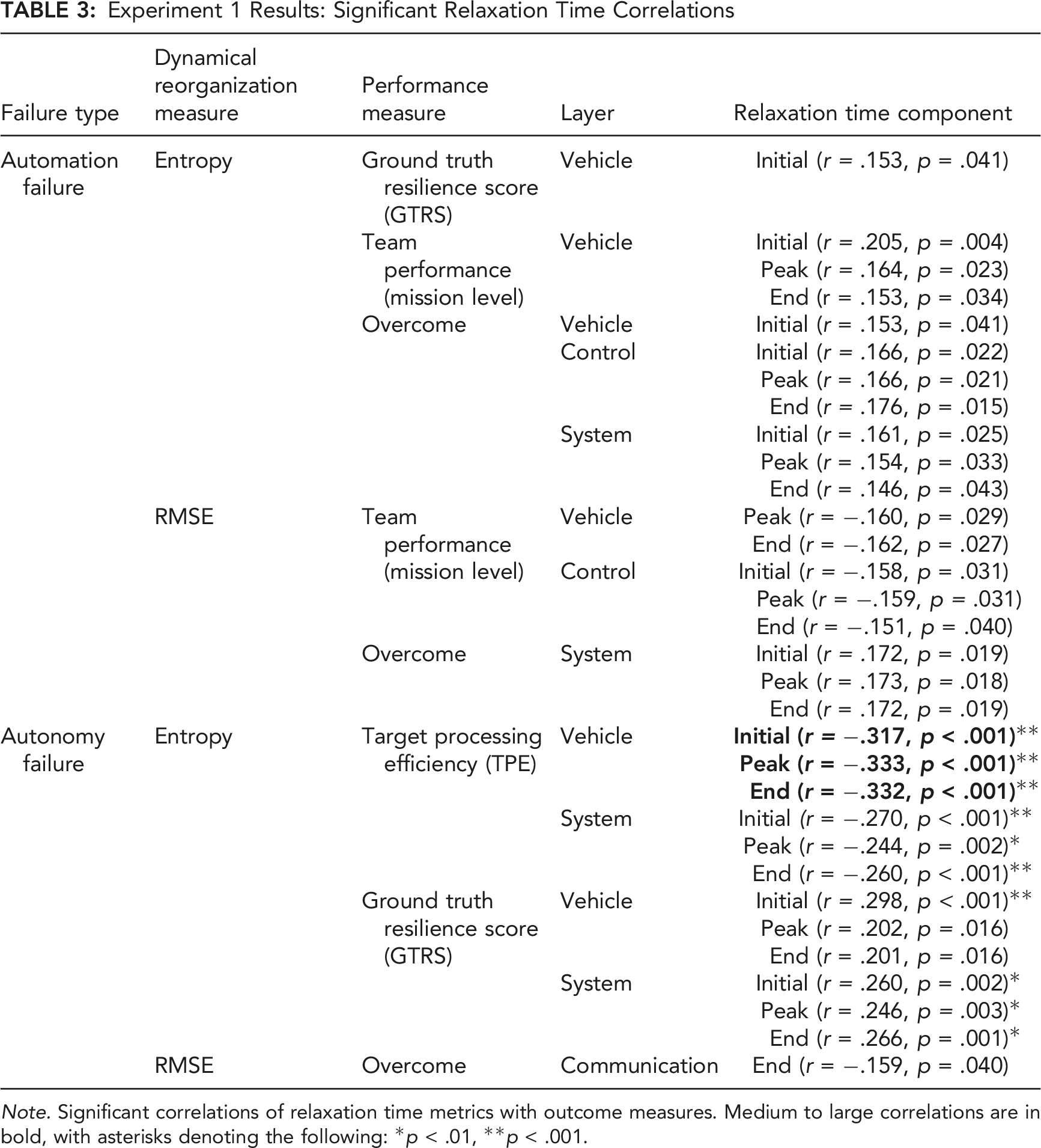
Note. Significant correlations of relaxation time metrics with outcome measures. Medium to large correlations are in bold, with asterisks denoting the following: *p < .01, **p < .001.
Using this criterion, all three relaxation time components were negatively correlated with TPE in the vehicle layer during autonomy failures, with the system layer falling just below our practical significance criterion (all |r| > .24). Thus, the vehicle and to some degree the system layer produced consistent correlations in the hypothesized direction for autonomy failures, whereas the results across all other system layers were less consistent. These results provide some support for E1.H1, that faster relaxation times would be correlated with greater team performance, across all three relaxation time components (Initial, Peak, End). The positive vehicle and overall system correlations were also sizable with respect to GTRS for autonomy failures.
Hypothesis E1.H2
Hypothesis 2a was that teams would display greater reorganization during failure perturbations compared to routine mission segments, and Hypothesis 2b was that this effect would be larger for more effective teams. To test this hypothesis, we calculated average system layer entropy separately for routine, automation failure, and autonomy failure segments of each mission. We obtained n = 788 average entropy values (9 missions × 22 teams × 4 layers; four observations were missing due to a file that failed to save) for each level of failure status (routine, automation, autonomy). To test the team effectiveness hypothesis (H2b), we clustered (k-means) teams on TPE, Team Performance, and Overcome, to classify low, medium, and high-performing teams across the three performance scores. We then analyzed mean entropy using a 3 (Performance Cluster [Low, Medium, High]) × 3 (Failure Status [Routine, Automation, Autonomy]) mixed Analysis of Variance (ANOVA), with Performance Cluster as a between-subjects factor and Failure Status as a within-subjects factor.
The main effect of Failure Status was significant, F (1.78, 1237.56) = 49.45, p < .001, Main effect of Failure Status on reorganization behavior (% max entropy) in Experiment 1. Error bars represent standard errors.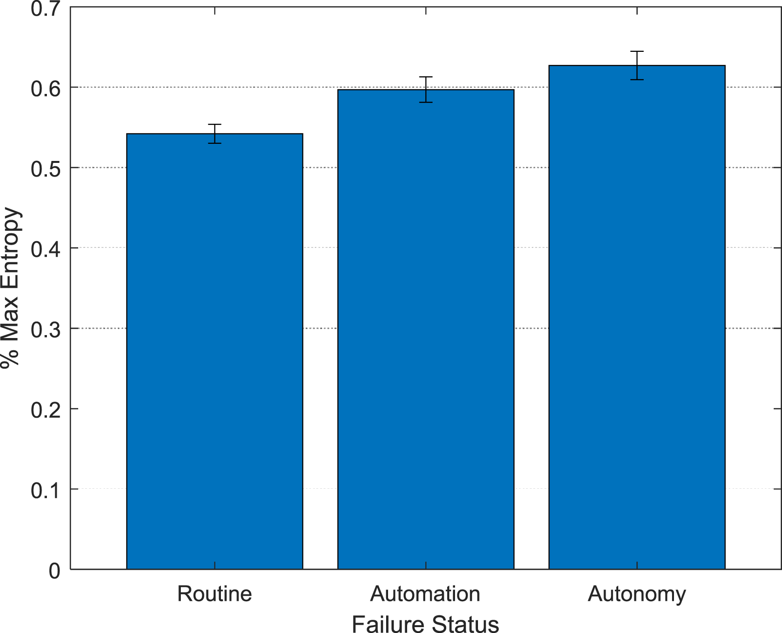
Hypothesis E1.H3
Sample Data Points for Target Processing Efficiency (TPE) Scores on Autonomy Failures to Illustrate the Generation of Large and Small Ground Truth Resilience Scores (GTRS)
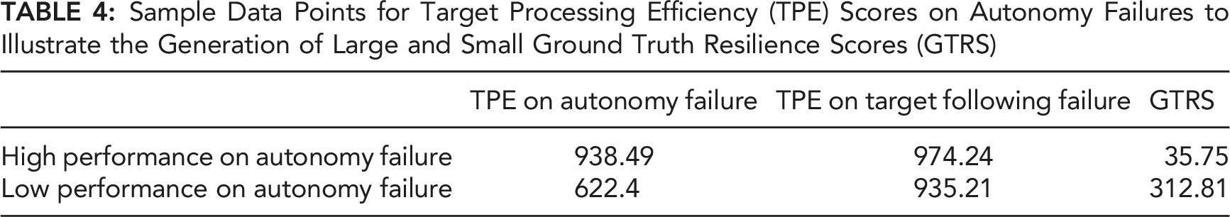
Considering that shorter relaxation times were generally correlated with higher TPE (Table 3), Figure 8 illustrates the empirical relationships underlying the positive correlation between relaxation time and GTRS. This positive correlation undergirds two interpretations of resilience in the current study, resilience as robustness and resilience as recovery (Woods, 2015). Graph of the relationships between relaxation time, target processing efficiency (TPE), and ground truth resilience score (GTRS) underlying the interpretation of resilience as robustness versus recovery.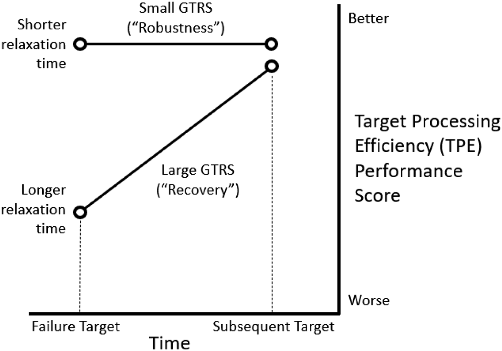
Experiment 2
Experiment 1 revealed that the dynamical systems resilience metrics were more sensitive to autonomy failures versus automation failures, in terms of the resilience-performance correlations. Experiment 1 also indicated separate interpretations of resilience using the metrics: resilience as robustness versus resilience as recovery and that the reorganization profiles suggested that autonomy failures required greater reorganization than automation failures, which in turn required greater reorganization than routine mission segments. Taken together, these results suggest that although they were of similar time durations (i.e., all failures were 420 sec except for Automation Type I, which was 300 sec), autonomy failures may have been more complex than automation failures, in that they required greater amounts of system reorganization by the team. Experiment 2 further investigates this effect by introducing even more complex failures in the form of hybrid automation-autonomy failures, system power-downs, and malicious cyberattacks. Experiment 2 was also designed to test separate training strategies for increasing resilience to automation and autonomy failures, providing the opportunity to examine the sensitivity of the dynamical systems resilience metrics to differences in team training.
Participants
Sixty participants (30 teams) between 18 to 33 years of age (M = 22.6, SD = 3.61) were recruited from Arizona State University and surrounding areas. The sample had a gender distribution of 52 males and 7 females, with one participant not responding. Ten teams were randomly assigned to each of the training conditions. Participants were required to have normal or corrected-to-normal vision and fluency in English. All participants were compensated $10 per hour.
Procedure
Experiment 2 took place over one session. As in Experiment 1, it used the WoZ paradigm in the CERTT-RPAS-STE with a trained experimenter in the synthetic pilot role and participants randomly assigned to either navigator or photographer. Participants were told that they were working with a synthetic teammate. Like Experiment 1, the experimenter was in a separate room, with the participants located in another room and separated by a partition.
Training Condition Manipulations
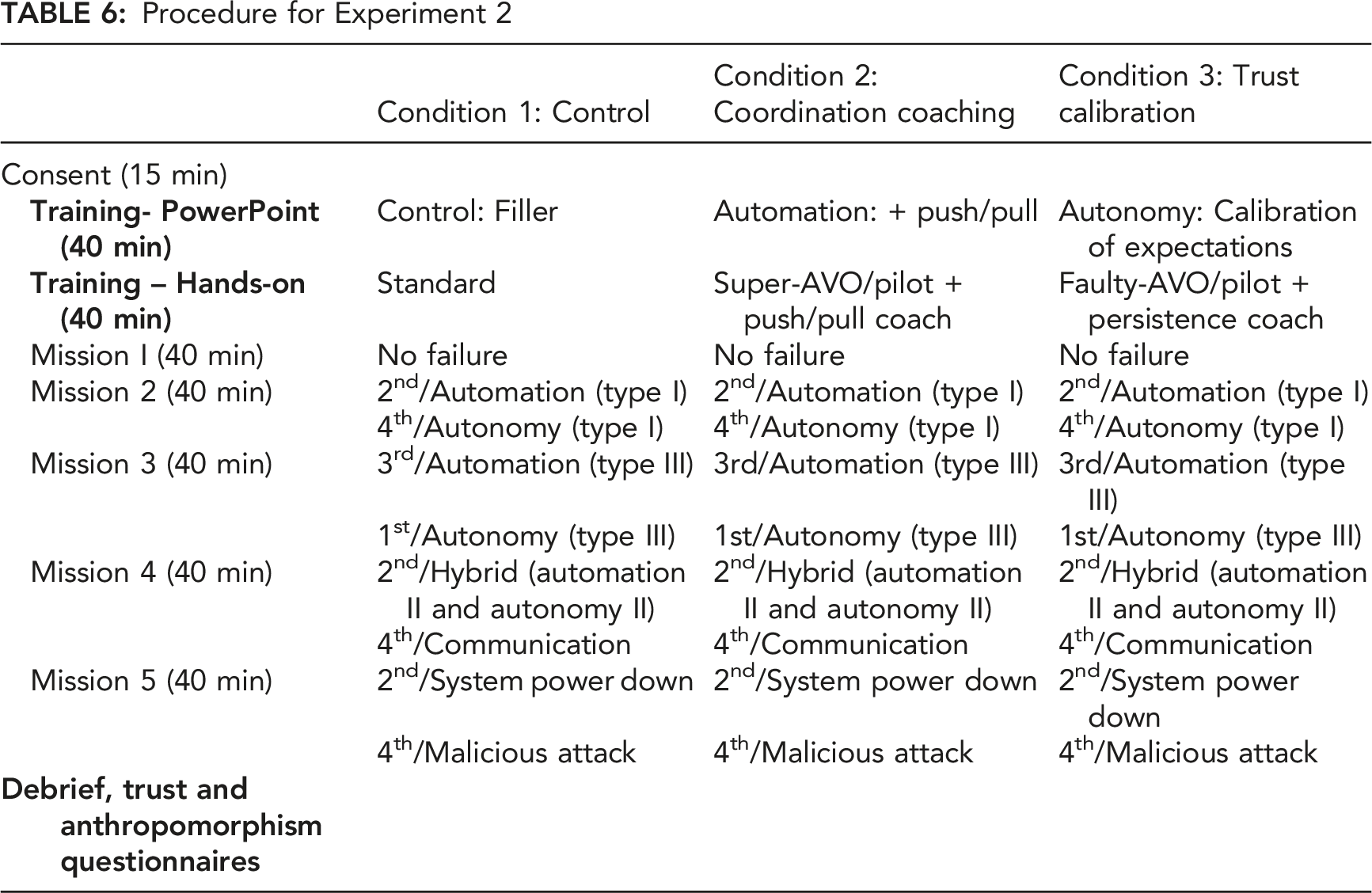
Procedure for Experiment 2
Failure Types
Experiment 2 included Automation Type III and Autonomy Type III failures as previously described. Other failures included malicious cyberattacks, hybrid failures, system power down failures, and communication cuts.
Malicious Cyberattacks
Malicious cyberattacks, introduced during the final 10 minutes of the final mission, simulated the synthetic agent being hijacked through cyberattack resulting in the agent providing false information detrimental to mission completion. In addition, the synthetic agent pilot attempted to fly the RPA to an enemy-designated waypoint. To overcome this failure, either the navigator or photographer had to explicitly inform Intelligence (an experimenter) that the RPA was off-route and was flying toward an enemy-designated area via chat message.
Hybrid Failure
The hybrid failure was a combination of the Type II automation failure and Type II autonomy failure from Experiment 1. The Type II automation failure affected the pilot, wherein the pilot was not able to view the altitude and airspeed for the next target and had to communicate with the navigator and photographer to achieve proper airspeed and altitude. The Type II autonomy failure portion was an anticipation failure, wherein the pilot began flying to the next waypoint before the photographer could take a photo of the target waypoint. To overcome this failure, the team needed to negotiate the proper settings with the synthetic pilot (Johnson et al., 2020). Since this is a combination of an automation and autonomy failure, the solution would naturally be a combination of solutions to these specific failures as described in Experiment 1.
System Power Down Failure
This failure simulated a system power down and rebooting during the mission. During this failure, there was a gradual power down of all screens over the course of 330 sec. The screens were powered down in order from pilot→navigator→photographer. After each team member lost their common information screen, the sequence repeated with each team member losing their role-specific screen. The screens then rebooted in reverse order. The photographer was still able to take a successful photo (until the last screen lost power) if the team adapted in a timely manner to ensure that all necessary information was provided to the affected team member before losing power.
Communication Cut Failure
In the communication cut failure, communication from the photographer to the pilot was cut; however, the pilot to photographer link remained active. Because the pilot’s communication links to the photographer and navigator remained intact, the pilot was unaware of the communication cut. To overcome this failure, the photographer had to communicate through the navigator to relay information to the pilot.
Results and Discussion
Hypothesis E2.H1
Experiment 2 Results
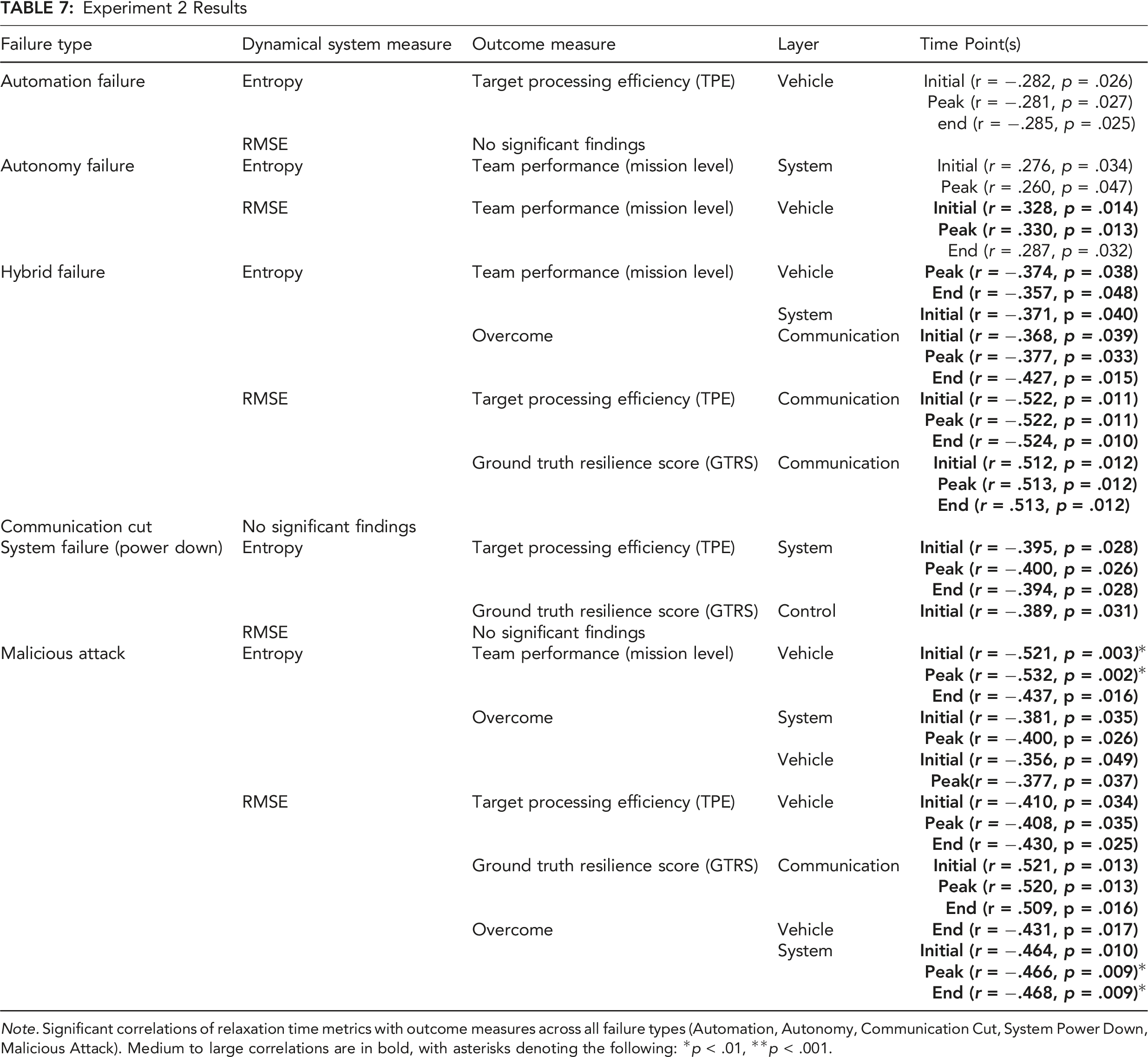
Note. Significant correlations of relaxation time metrics with outcome measures across all failure types (Automation, Autonomy, Communication Cut, System Power Down, Malicious Attack). Medium to large correlations are in bold, with asterisks denoting the following: *p < .01, **p < .001.
As in Experiment 1, although significant, the automation failure correlations did not meet the medium-to-large effect size criterion. In addition, the communication cut correlations were not significant. All performance correlations were in the hypothesized direction except for the autonomy failure, for which we found positive correlations between relaxation time in the vehicle layer for team performance. Unlike the performance measures that correlated in the hypothesized direction (i.e., Overcome and TPE), the team performance outcome measure was taken at the mission-level rather than the failure target level, perhaps contributing to this unexpected result. As indicated by the changing patterns of medium to large correlations across system layers and failure types, these results suggest that specific patterns of relaxation times and system reorganization across system layers depend on failure type. The positive correlations between relaxation times and GTRS replicated the finding from Experiment 1 and are discussed later, under Hypothesis E2.H3.
Hypothesis E2.H2
Hypothesis 2a was that teams would display greater reorganization during failure perturbations compared to routine mission segments, and Hypothesis 2b was that this effect would be larger for higher-performing teams. We carried out the same analysis as for Experiment 1 by conducting a k-means cluster analysis to identify low, medium, and high-performing teams, calculating average entropy according to failure status, and running a mixed ANOVA on the average entropy values. We obtained n = 348 average entropy values (29 teams × 4 layers × 3 failure complexity [described below]; one team was missing due to a file that failed to save). The Experiment 2 analysis also included Training Condition as a between-subjects factor. Because each mission had two failures (Table 6), we classified the various failure types as Failure One and Failure Two, constituting a within-subject variable, Failure Status. We analyzed the average entropy scores using a 3 (Performance Cluster [Low, Medium, High]) × 3 (Failure Status [Routine, Failure One, Failure Two]) × 3 (Training Condition [Control, Coordination Coaching, Trust Calibration]) mixed ANOVA. Due to the different failure types included in the Failure One and Failure Two factor, we included a covariate, Failure Complexity, that indexed the different possible failure combinations.
There was a main effect of Failure Type, F (1.702, 549.762) = 17.373, p < .001, The main effect of Failure Type in Experiment 2 shows that failure perturbations resulted in greater entropy (reorganization) compared to routine mission segments. Failure 2 entropy was also significantly greater than Failure 1 entropy. Error bars represent standard errors.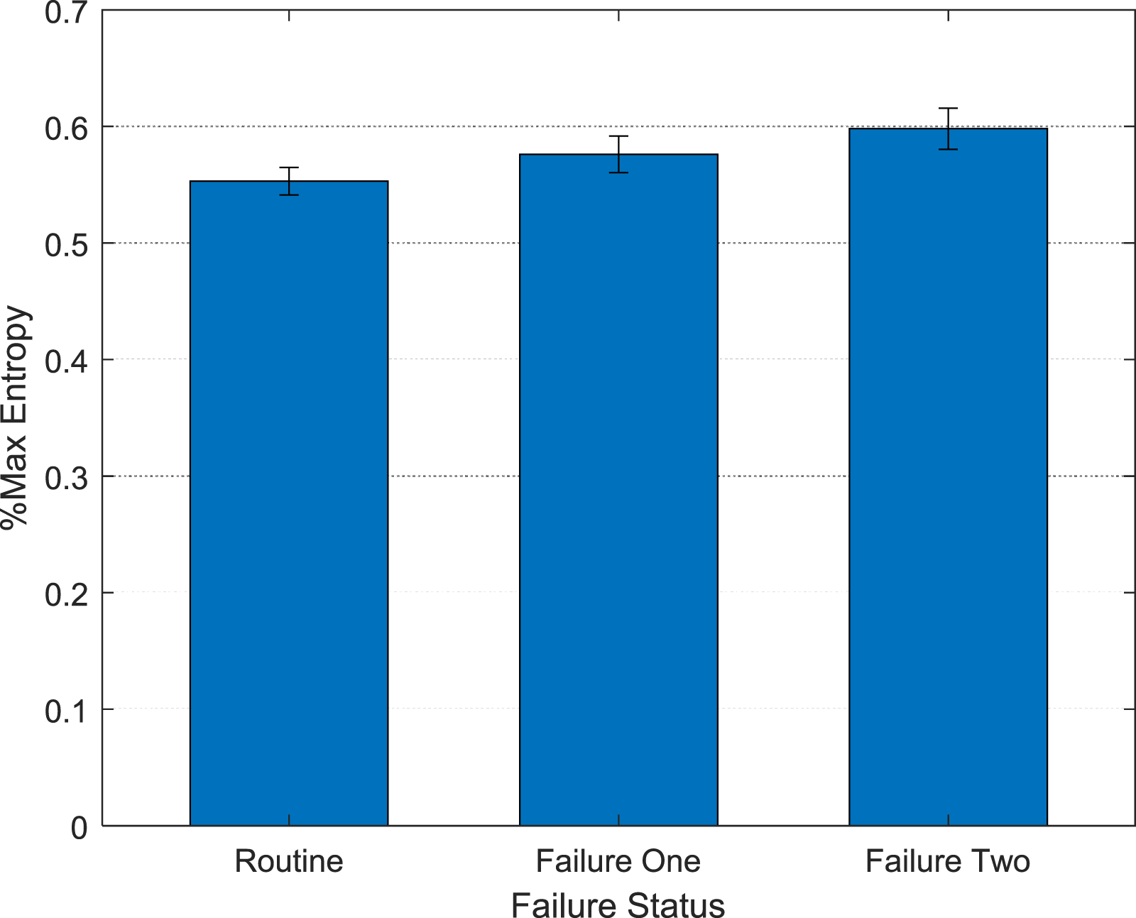
The Failure Status × Failure Complexity (covariate) interaction was significant, F (1.690, 544.262) = 18.587, p < .001, The amount of reorganization (entropy) differed as a function of failure type, with autonomy failures producing the greatest amount of entropy. Error bars represent standard errors.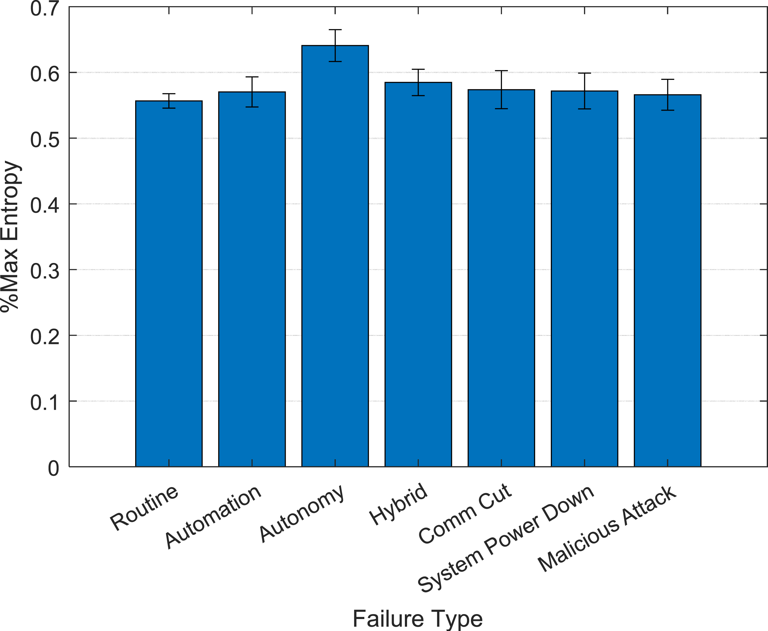
Hypothesis E2.H3
Sample Data Points for Target Processing Efficiency (TPE) Scores on Hybrid Failure and Malicious Attack to Illustrate the Generation of Large and Small Ground Truth Resilience Scores (GTRS)
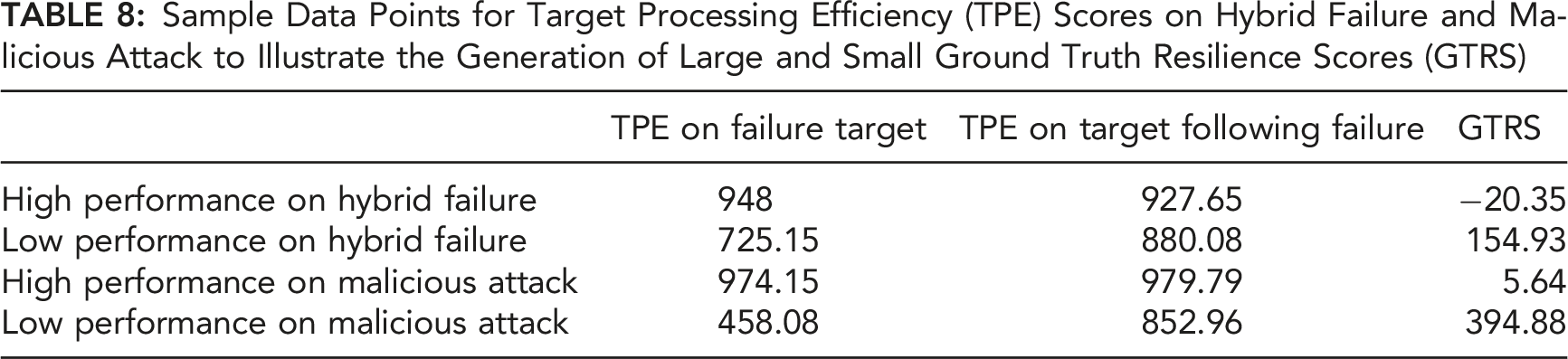
The pattern of TPE scores in Table 8 predicts a strong, negative correlation between failure target TPE and the resulting GTRS, due to the mapping of high TPE on the failure target onto small GTRS (“robustness”) and low TPE on the failure target onto large GTRS (“recovery”). Another possibility that must be accounted for is that low TPE on both the failure target and the follow-up target (“non-resilient”) can result in small GTRS. In that case, we would expect a smaller, insignificant correlation between TPE on the failure target and GTRS, due to the inconsistent mapping between TPE failure target score (equal mix of high and low TPE) onto GTRS. Indeed, the correlations between TPE on the failure target and GTRS were strong and negative for both the Hybrid Failure, r (21) = −.669, p < .001, and Malicious Attack, r (20) = −.755, p < .001, indicating that our results were primarily due to a mix of the robustness and recovery forms of resilience. This same pattern of correlations between TPE and GTRS was observed across experiments, despite the different experimental manipulations across the two experiments. As explained later (Table 11), low GTRS scores resulting from the “robustness” pattern of TPE scores were approximately 47% more frequent than low GTRS resulting from the “non-resilient” pattern of TPE scores across both experiments.
Hypothesis E2.H4
Experiment 2 Training Effect Correlations
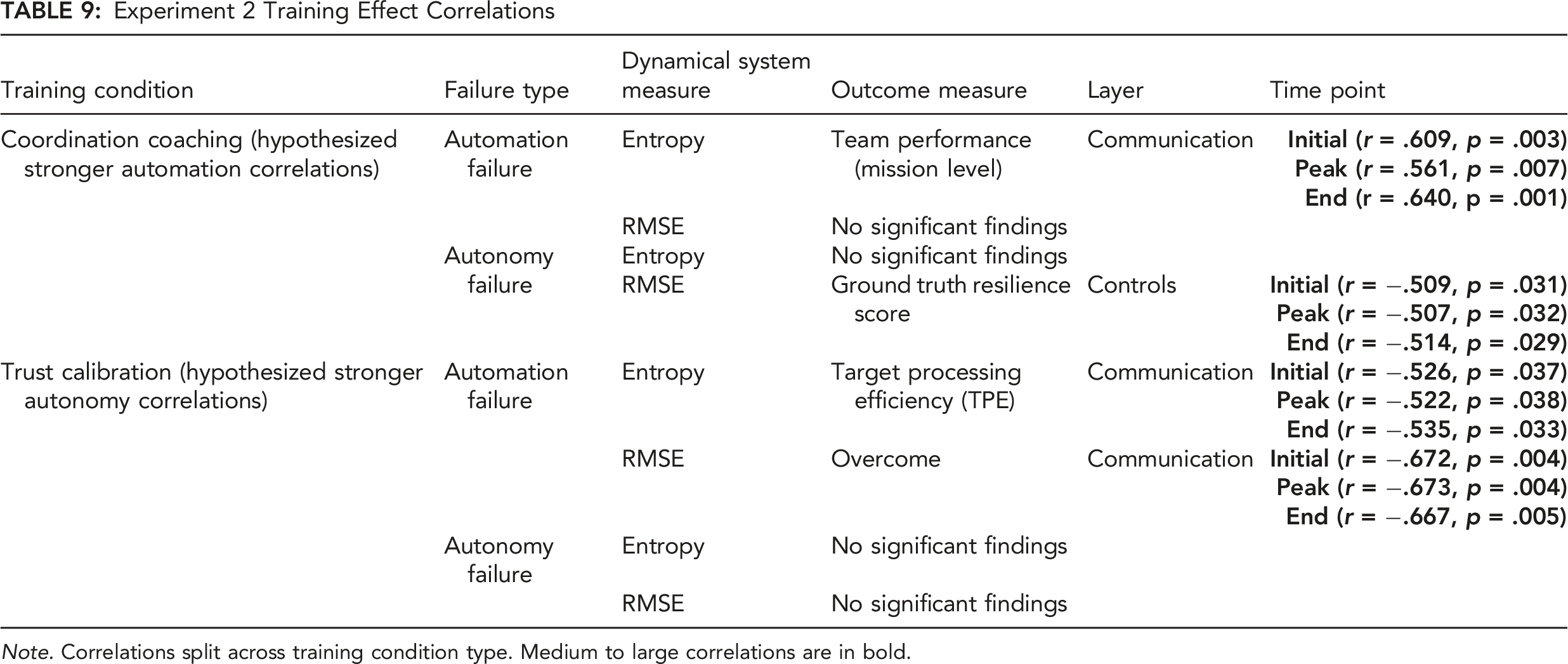
Note. Correlations split across training condition type. Medium to large correlations are in bold.
Summary of Findings Across Experiments 1 and 2
General Discussion
Although they may occur infrequently compared to routine conditions, failure perturbations are to be expected in dynamic HAT environments. These are often high-stakes, one-of-a-kind events that require enaction, adaptation, and recovery by HATs. The current studies developed and tested a novel approach for measuring HAT resilience in a controlled laboratory setting. We envision, however, that versions of these metrics will be deployed in operational environments, wherein team adaptation and resilience are critical for safe and effective operations. Based on the current results, these metrics are promising as real-time indicators of when and how HATs resolve failure perturbations.
Consistent with Hoffman and Hancock’s (2017) theoretical resilience measurement model, we operationally defined three components of a “resilience curve” (Figure 5), comprising initial (“enaction”), peak (“adaptation”), and final (“recovery”) relaxation time components. Considering only medium-to-large relaxation time-performance correlations, we found support for the hypothesis that relaxation times were negatively correlated with better team performance (Hypothesis 1) across both experiments. These results suggest that faster enaction, adaptation, and recovery during failures predict greater team effectiveness. Although the preponderance of correlations supports this hypothesis, mission-level team performance and GTRS (discussed below) indicated positive correlations. Regarding mission-level team performance, this performance measurement was taken at the mission level, whereas the other measures were taken during and just after a failure at the target-level. The mission-level performance score also included the amount of time spent in warning or alarm states. It is possible that faster relaxation time coupled with less time spent in warnings or alarms over the whole mission could account for the positive correlation with mission-level performance.
One potential difficulty with relaxation time metrics is that as failures become increasingly complex (e.g., moving from Experiment 1 to Experiment 2), the locus of resilience (e.g., system layer) may be difficult to predict. In Experiment 1, correlations were found primarily in the vehicle and system layers, whereas in Experiment 2, correlations were found in all system layers. This may reflect the bespoke nature of adaptation and resilience to increasingly complex system failures. Although currently our resilience metrics have the advantage of identifying where and when a system reorganizes across system layers, there is no simple law relating system layers to failure complexity. This may still be a potential benefit to resilience engineering, however, which views teams as large systems containing numerous components with complex interactions that are difficult to predict in perturbed operational settings (Hollnagel et al., 2007). We argue, therefore, that this approach can help identify, if not predict a priori, which system layers are key to resilience in dynamic environments.
There is, however, a straightforward law that relates the amount of reorganization to the variety demanded by the environment in terms of maintaining stable system performance, the law of requisite variety (Ashby, 1957). In both experiments, we found support for the hypothesis (Hypothesis 2a) that teams would display significantly greater reorganization behavior during failures compared to routine (nominal) mission segments, regardless of the source (system layers) of reorganization. We additionally hypothesized that this effect would be greater for more effective teams (Hypothesis 2b), such that teams with higher performance scores would exhibit larger differences between failure and routine reorganization. We did not find support for the latter hypothesis. However, the point of this law is that a controller must be able to match the variety required by the system it controls. The question is whether it is effective in doing so. For instance, a poorly designed traffic system takes longer to match the same amount of requisite variety compared to an effectively designed traffic system. In the current study, all HATs were exposed to the same amounts of requisite variety. However, as demonstrated by the relaxation time metrics and support for Hypothesis 1, timeliness of response was key, over and above the amount of variety the system can match. Although not observed in the current studies, it should be noted that Ashby’s Law is a key contribution to the inverse-U relationship between controller complexity and performance. This means that if there is too much complexity in the controller, then there is wasted effort, which can be a detriment to a team’s efficiency (Boisot & McKelvey, 2011; Friston, 2010; Guastello, 2015; Hong, 2010).
In support of the hypothesis that relaxation times would predict ground truth resilience (GTRS; Hypothesis 3), we found medium to strong correlations between relaxation times and GTRS, largely in the positive direction, in both experiments. Moreover, shorter relaxation times (i.e., faster enaction, adaptation, and recovery) at the failure target were correlated with higher TPE at the failure target, indicating that resilience in the current studies can be interpreted as either robustness or recovery. This suggests that although resilience as recovery may contribute to resilience, it can also be associated with robustness, or the ability to handle increasing complexity at the point of the system failure (Woods, 2015).
Mode Resilience Profile Classifications Using Ground Truth Resilience Scores (GTRS) for Teams Across Experiments 1 and 2
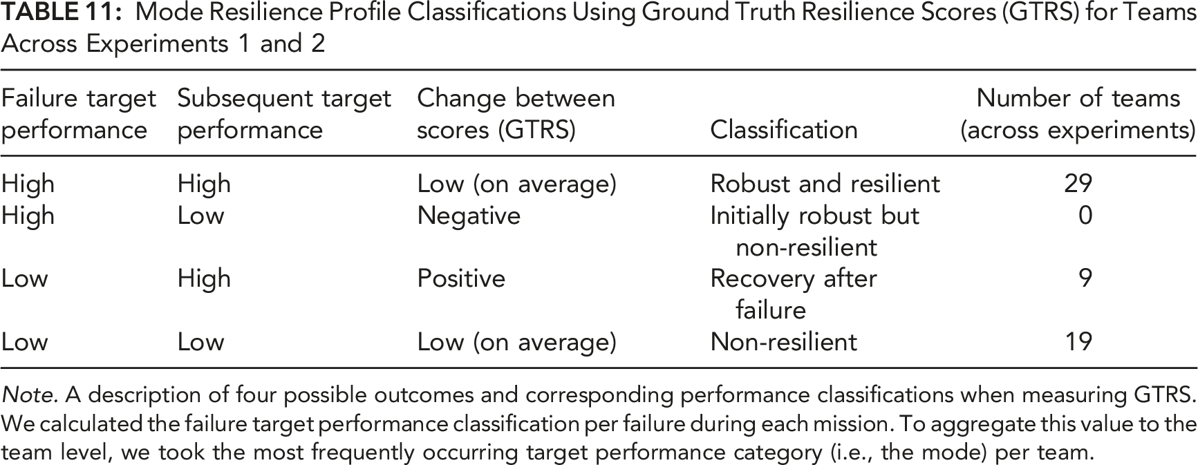
Note. A description of four possible outcomes and corresponding performance classifications when measuring GTRS. We calculated the failure target performance classification per failure during each mission. To aggregate this value to the team level, we took the most frequently occurring target performance category (i.e., the mode) per team.
A second possibility is that a team performed well on the failure target but performed poorly on the subsequent target. This team could be considered robust initially but possibly lacking in recovery after doing so, thereby failing to perform well on the follow-up target. It is possible, for example, that such teams may expend their energy on the failure target, making it difficult to function effectively afterwards. However, this pattern was not observed in the current studies (n = 0). A third possibility is that a team may perform poorly at the point of failure but performs well on the subsequent target. These teams would have a high GTRS and would be considered resilient in terms of recovery but not robustness. This pattern, which would account for the remainder of the negative correlation between relaxation time and GTRS, was not as frequently observed in the current studies (n = 9).
A final possibility is that teams perform poorly on both the failure target and the subsequent target. Teams in this category would be non-resilient from both a robustness and recovery perspective (Woods, 2015). This pattern, however, does not map onto the strong negative correlations between failure TPE and GTRS. Nevertheless, this pattern was observed in the current studies (n = 19), although 47% less often than the robust and resilient pattern, but it could contribute to positive correlations between relaxation time and GTRS. Thus, relaxation time metrics should be supported by classification metrics to disentangle the formal nature of team resilience. The approach used in the current studies could be implemented in real time using real-time TPE scoring. At a minimum, to create these profile classifications, one needs to examine not just the change scores, but the different performance classifications at both the point of failure and subsequent targets (e.g., Table 11).
These findings align with previous research in which teams competed against a sentient attacker (Guastello, 2010; Guastello et al., 2017). Like our studies, that research focused on dynamical systems metrics, which quantified adaptability and resilience using the largest Lyapunov exponent (an index of stability and chaotic behavior). When enemy attacks were making progress, team performance dropped both during the current performance opportunity as well as the subsequent performance opportunity, during which decision making was hampered. However, teams exhibited higher levels of adaptation compared to attackers as measured by larger values of their largest Lyapunov exponents.
With respect to our training hypothesis (Experiment 2, Hypothesis 4), results were mixed. Teams trained in the Coordination Coaching condition demonstrated strong relaxation time correlations when overcoming automation failures as hypothesized, although the direction of correlation (positive) was not in the predicted direction. These teams also demonstrated the hypothesized strong negative relaxation time correlation in response to autonomy failures, which was not hypothesized. Teams trained in the Trust Calibration condition did not demonstrate the hypothesized strong relaxation time correlations when overcoming autonomy failures; however, they did demonstrate strong negative relaxation time correlations when overcoming automation failures, which was not hypothesized. Interestingly, these training effects were most apparent in the communication layer and to a lesser extent in the controls layer. Consistent with other analyses of these training effects demonstrating that coordination training primarily impacts communication, this implies that communication reorganization may be critical when overcoming failures of increasing complexity, and that the relationship between communication reorganization and performance differs depending on training condition (Johnson et al., in press). Overall, Coordination Coaching teams appear to be more resilient in terms of their relaxation time—performance relationships because these relationships were observed for both automation and autonomy failures, whereas Trust Calibration teams only demonstrated these relationships for automation failures.
Given the many definitions of resilience in the literature (Hollnagel et al., 2007; Woods, 2015), as well as recommendations to practitioners on how to apply concepts of resilience engineering in practice (Hollnagel, 2013), there is currently a lack of methods for objectively measuring team resilience in dynamic sociotechnical environments. However, layered dynamics and relaxation time metrics demonstrate the potential for objective, real-time methods that can be used to quantify resilience across system layers that are predictive of various aspects of team performance. The current approach builds on the work of Hoffman and Hancock (2017), who proposed a theoretical approach for measuring resilience. We submit that their proposal, which comprises recognition, design, and implementation of system changes in response to failures, aligns with the operational definitions of enaction (Initial), adaptation (Peak), and recovery (Final) relaxation time metrics that comprise a “resilience curve” in the current studies. Although we do not claim a strict, one-to-one match with their proposed theoretical framework, the concept of measuring resilience as the capacity to overcome a failure and rapidly and efficiently recover to a stable state, we claim captures the essence of their theoretical approach.
The current results may further be tied to theoretical concepts in resilience engineering. Woods (2015) defines four concepts of resilience, including resilience as robustness, resilience as rebound from degraded conditions, resilience as graceful extensibility, and resilience as sustained adaptability. The current results most directly apply to the first three. In relation to ground truth resilience (e.g., GTRS), we argue that relaxation time can be indicative of robustness (performance on both targets is high) or low-performing, non-resilience (performance on both targets is low) when the correlation is positive and rebound or recovery when negative. Thus, relaxation times are indicative of different theoretical conceptualizations of resilience depending on the robustness of the system and its ability to recover from a failure. The third concept, graceful extensibility, is the ability of a system to extend its capacity in response to novel disturbances. Although we did not aim to directly measure this property in the current studies, the “extensibility” component of this property is arguably represented by the consistently greater system reorganization values observed under failure conditions compared to routine conditions. The “graceful” component may be embedded within the relaxation time—performance correlations, which should be explored in future research. Overall, the aims of the current research involved generating dynamic systems-based resilience metrics, wherein rapid reorganization tends to be associated with better performance, and sublayers can be used to identify the sources of rapid responses and resilient behavior within a system. On those counts, the current results are promising for future applications of these metrics in training and operational settings.
Limitations and Future Directions
Although we can generally argue that relaxation time metrics measure robustness, recovery, and extensibility, due to the number of system layers, types of failures, relaxation time metrics, and performance measures, there were a very large number of correlations, making a clean interpretation of the results difficult. In the future, it may be beneficial to use a less complicated experimental apparatus with fewer layers and types of failures to parse out the causal relations between perturbations and relaxation times as they relate to resilience. Although it would appear to bely the bespoke nature of unique events that require resilience, a more highly controlled and simpler experiment might help unpack the complex dynamics observed in the current studies.
Additionally, more conceptual work is needed on the two dynamical system measures used, entropy (reorganization) and RMSE (novelty), and how they meaningfully relate to system response. Entropy describes system response in terms of the number of unique states occupied by the system during a span of time. Currently, we think this is analogous to variety in Ashby’s (1957) law of requisite variety. On the surface, RMSE captures the novelty of system response in terms of the deviation from a predicted trajectory of the reorganization time series. However, RMSE is agnostic as to the source of a novel trajectory of the entropy time series. Moreover, because it is a square root, RMSE, in terms of novelty, could correspond to extremes of either increasing or decreasing variety. Future work should focus on more exactly tying novel team states to requisite variety that maintain system effectiveness under degraded conditions.
Along these lines, future directions in resilience measurement could disentangle these two metrics based on their respective explanations of a system response. Thus, another future direction involves selectively filtering out sources of variation, such as team members or sublayers, to identify which are critical for reorganization and novelty in a team response (e.g., by using the filtering method described in Gorman et al., 2020). For example, one could filter the control layer from the overall system layer separately for the reorganization and novelty metrics to determine if significant correlations between relaxation time and performance persist across other layers.
Finally, it is worth noting that the relaxation times do not necessarily indicate whether a system is revisiting a previous state, or if it is moving into a new state. Our metrics quantify reorganization and resilience by computing unique states of the system, but they do not currently capture qualitative differences among those states. In this light, there are other metrics available for quantifying resilience based in dynamical systems theory that are relevant to this line of research (Guastello & Gregson, 2011).
Conclusion
The methodological approaches described in the current paper have the potential to impact the training and assessment of HATs as well as teams in other sociotechnical contexts. These environments can be highly dynamic and are susceptible to system failures, errors, and crises. This work is beneficial in many situations in which team flexibility, preventive behavior, and resilience are critical, and real-time metrics are needed. The metrics developed in this work have strong potential for real-time implementation that would benefit the training of more resilient teams and the design of more resilient systems by providing real-time feedback and guidance during training and simulation, as well as understanding how systems reorganize to maintain high levels of effectiveness during one-of-a-kind, anomalous events (e.g., Gorman et al., 2020; Grimm et al., 2017). Real-time analysis of reorganization and resilience may also enable analysts and operators in operational environments to detect early onset of maladaptive and possibly dangerous team actions. Taken together, we propose that these types of measures will inform and generate new approaches to teamwork measurement, monitoring, and assessment strategies in sociotechnical work domains in which timely and resilient responses are critical.
Footnotes
Acknowledgments
We acknowledge Paul Jorgeson and Steve Shope for their assistance modifying the CERTT-RPAS-STE; John Flach for contributing to our understanding of requisite variety; and Cody Radigan, Craig Johnson, Sophie He, Matthew Lin, Tanvi Tandolkar, Garrett Zabala, Alexandra Wolff, for data collection efforts. Lastly, we acknowledge Dr. Ronald H. Stevens for inspiring the methodological approaches described in this paper.
Declaration of Conflicting Interests
The author(s) declared no potential conflicts of interest with respect to the research, authorship, and/or publication of this article.
Funding
The author(s) disclosed receipt of the following financial support for the research, authorship, and/or publication of this article: This research was supported by ONR Award N000141712382 (Program Managers: Marc Steinberg; Micah Clark).