Sage Journals: Discover world-class research

Abstract

There are much data transmitted from sensors in wireless sensor network. How to mine vital information from these large amount of data is very important for decision-making. Aiming at mining more interesting information for users, the skyline technology has attracted more attention due to its widespread use for multi-criteria decision-making. The point which is not dominated by any other points can be called skyline point. The skyline consists of all these points which are candidates for users. However, traditional skyline which consists of individual points is not suitable for combinations. To address this gap, we focus on the group skyline query and propose efficient algorithm to computing the Pareto optimal group-based skyline (G-skyline). We propose multiple query windows to compute key skyline layers, then optimize the method to compute directed skyline graph, finally introduce primary points definition and propose a fast algorithm based on it to compute G-skyline groups directly and efficiently. The experiments on the real-world sensor data set and the synthetic data set show that our algorithm performs more efficiently than the existing algorithms.

Keywords

Wireless sensor network skyline multi-criteria group-based skyline multiple query windows primary points

Introduction

Wireless sensor network (WSN) is a kind of distributed sensor network, whose terminal is the sensors that can sense and check the external world. WSN uses sensors to collect information in the detection area and transmits data through wireless communication. Therefore, a lot of data can be collected through WSN, so how to mine vital information from these mass data for special purpose is very important.

As one of the important query mining techniques, skyline query¹ can return all the Pareto optimal points that are not worse than any other points in the same data set, and it is very useful in many applications, such as data mining and multi-standard decision-making. Although which points in skyline are selected depend on user’s decision and other factors, after all, skyline query reduces the size of the outstanding candidate set by pruning the mediocre points.

Assume there is a data set P of n points with d dimensions, p and q are two distinct points in P, we can say p dominates q, if p[i] <= q[i] for each i and at least p[j] < q[j] (1 ≤ i, j ≤ d), where p[i] indicates the value of p in the ith dimension. The skyline of data set P consists of all the points which are not dominated by any other points in P. We can say the skyline indicates the Pareto optimal points as the skyline points are better points and cannot dominate each other.

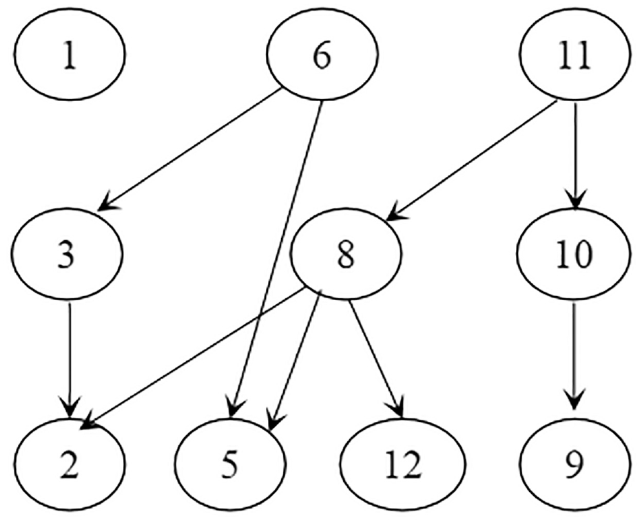
Take a case in forest fire warning system, for example, aiming at detecting fire hazard, thousands of sensors connected via a WSN are deployed throughout the forest. When the fire is about to burn or has broken out started, the nearby humidity will decrease, and the nearby temperature will increase sharply. As shown in Figure 1(a), there are 12 points in data set P, and each point represents a sensor with two attributes: the humidity and the inverse-temperature. The suspicious point with smaller humidity and inverse-temperature can be returned by skyline query on data set P, so the forest fireman can run to these skyline points to check for fire hazards. In this case, we find three points should be checked as soon as possible, p₁, p₆, p₁₁, as these three dangerous points have smaller humidity or/and inverse-temperature. These three points are skyline points of P, as shown in Figure 1(b).

Figure 1.

An example of skyline: (a) data set P and (b) skyline.

Motivation

In the above example, due to the limitation of fire fighting force, in order to effectively control fire hazards, the most effective method is to patrol some suspicious sensors in groups. If we planned to divide the fire forces into teams, each of which would patrol three trouble sensors as a group, traditional skyline queries would not be able to satisfy the demand. As the traditional skyline query can only return results in units of individual point, it is deficient for user to do query based on groups or combinations. In fact, this query is very practical and often used in WSN environment.

To remedy this deficiency, group-based skyline (G-skyline for short) query² is proposed to return candidate set which consists of better groups containing k points. This query is more useful than traditional skyline query in many applications which need to return some better groups from data set, such as sensors wireless network, data mining, and multi-criteria decision. In the above example, if there are four fire force teams and each plans to patrol two trouble spots once a time, we can do G-skyline query with two points, the result is {p₁, p₆}, {p₆, p₁₁}, {p₁, p₁₁}, {p₁₁, p₃}, {p₁₁, p₁₀}, {p₁₁, p₈}, so the fire force can select some groups from result for patrolling based on actual situation, and the query result can support the decision.

Although some existing algorithms can do group skyline query, they either need too much computation³ or cannot get complete candidate groups.^2,4 G-skyline is a complete candidate set since it contains all Pareto optimal groups, but a time-consuming algorithm returning an oversized candidate set is far from practical.³ The group skyline with specific function can only return the result corresponding to the function, but it cannot contain all Pareto optimal groups.⁴ So a complete and efficient algorithm is needed urgent.

Contributions

We summarize our main contributions in brief as follows.

We define the key skyline layers which are necessary for computing G-skyline and present a new method based on multiple query windows to compute key skyline layers efficiently.

We optimize the structure of directed skyline graph (DSG) and present a new method to construct DSG with less comparison.

We propose a fast algorithm to compute G-skyline. We define the primary points which play a major role in G-skyline and prove some key rules to prune useless data, then propose an efficient algorithm to compute group-based skyline as mentioned earlier.

The experiments are performed based on the real-world sensor data and three kinds of synthetic data.

Organization

The rest of this article is organized as follows. In section “Related works,” we review the related works to our research work. In section “Key skyline layers,” we give some basic definitions and theorems, define the key skyline layer, and present a new method to build it. Section “Directed skyline graph optimization” presents the optimized DSG and the algorithm to construct it. Section “Computing G- skyline groups” presents key rules and the efficient algorithm to computing G-skyline. Section “Experiments” shows the experimental results by comparing our algorithm with other existing algorithms. At last, we conclude our research work in this article and propose the future work.

Related works

In this section, the previous related work on skyline query is explored. After Borzsonyi et al.’s¹ original work to present the skyline operator in 2001, lots of researchers have done much work on skyline query in many filed, so many methods about skyline have been presented for different problems.

In article,¹ Borzsonyi presented BNL algorithm and D&C algorithm which were first to do skyline query. SFS⁵ returned the skyline result by sorting the data set according to the monotone function. Bitmap⁶ computed skyline by querying vectors mapped from points in data set. In NN⁷ algorithm, the nearest neighbor points were filtered to compute the skyline result. Liu et al.⁸ proposed a query window to compute skyline efficiently by pruning most useless data.

Besides, variants of improved skyline algorithms for the specific applications were presented. The sub-space skyline^9–11 can return skyline based on user’s different preference. K-dominant skyline^12,13 can return the candidate points when the points dominate each other with difficulty. Top-k skyline^14–18 returned the first k points in ranking by a function, and it was suitable for queries that have specific requirements for the number of results. Kim et al.¹⁹ and Zaman et al.²⁰ introduced MapReduce technology to do skyline query on distributed database efficiently. Not only that the probabilistic skyline^21–23 was also presented to do query on uncertain data set which was different from data set in above algorithms. Previous articles^24–27 proposed the skyline query in data stream in which the points had lifetime. Li et al.²⁸ studied the skyline query based on a road-social network consisting of a road network and a location-based social network.

Few articles^4,29–32 discussed different skyline applications in WSNs, such as continuous reverse skyline, spatial skyline, distributed dynamic skyline, and probabilistic skyline query in the WSNs.

In recent years, group-based skyline query has been focused on by researchers increasingly.^{3,4,28,33–41} Previous articles^33–36 computed top-k composition skyline. Few studies^37–39 did combination skyline query based on composition function, which computes the value of the same attribute of k points. In these methods, each k points can be regards as a virtual point with the same attributes of the source data, and the composition functions were usually simple aggregate functions, such as SUM, MAX, or MIN. Guo et al.⁴⁰ proposed skyline group algorithms with composition function in data stream based on the algorithms in articles.^37,38 Dong et al.⁴¹ proposed G-skyline query over data stream in WSN. Zhu et al.⁴ evaluated most existing algorithms based on two types of definitions in terms of time and space on various synthetic and real data sets.

However, there is an obvious flaw about such combination skyline query with function that is really hard to choose an exact composition function for group in practical application. In other words, the groups returned by these algorithms are not complete as not all Pareto optimal groups can be returned. In order to capture all Pareto optimal groups, Liu et al.² presented a new definition named group-based skyline (G-skyline), and it defined the dominance relationship between two groups by finding two permutations satisfying certain conditions. The G-skyline query can return all Pareto optimal groups which contain the result captured by previous algorithms with composition function. In fact, this method needs much computation and running time, so Yu et al.³ proposed an approach to do the search concurrently on each dimension and investigated each point in sub-space, then presented a structure to construct G-skyline. However, there is still much work to do to improve the efficiency of computing G-skyline.

Key skyline layers

In this section, we will explain the basic definitions and theorems, then we define and prove key skyline layers which are important for computing G-skyline and propose the efficient construction method later.

Definitions and theorems

Definition 1 (dominate)

Given a data set P, point p dominates point q if p is not worse than q in each dimension and p is better than q in at least one dimension, where p and q are in P.¹ We can use symbol “≺” to present “dominate.”

Definition 2 (skyline)

The skyline of data set P consists of all the points not dominated by any other points in P.¹

Definition 3 (g-dominante)

For two different groups G₁ = {p₁, p₂,…, p_k} and G₂ = {q₁, q₂,…, q_k} constructing from the same data set P, we can say G₁ g-dominates G₂, if two arrays with k points for G₁ and G₂ are found, G₁ = {p_n1, p_n2,…, p_nk}and G₂ = {q_m1, q _m2,…, q_mk}, and p_ni ≤ q_mi for each i (1 ≤ i ≤ k) and at least one j, p_nj dominates q_mj (1 ≤ j ≤ k).²

Definition 4 (G-skyline)

G-skyline is a set which consists of all the groups not g-dominated by any other groups with the same size.² We use G-skyline(k) to denote the G-skyline with group size k.

Example 1

The G-Skyline is Pareto optimal skyline, and it is different from traditional skyline, composition skyline,³⁹ or skyline groups.^4,38,40 In fact, the latter two case are same. We take an instance to illustrate the difference between G-skyline and them. In Figure 1, let G₁ = {p₆, p₈, p₁₁} and G₂ = {p₂, p₃, p₁₀}, according to g-domiante definition, we can find two enumerations {p₆, p₈, p₁₁} and {p₃, p₂, p₁₀} where p₆ dominates p₃, p₈ dominates p₂, p₁₁ dominates p₁₀, so we can say G₁g-dominates G₂; according to combination dominate definition,³⁹G₁={(8+20+16), (260+180+60)}= {44,500} and G₂={(14+24+28), (340+380+100)} ={66, 820} if we set SUM as combination function, we can say G₁ dominates G₂. However, if G₁ = {p₃, p₆} and G₂ = {p₁, p₁₁}, we can get that G₁ and G₂ do not g-domiante each other, but G₂ dominates G₁ if we set SUM as combination function. So we can see that G-skyline can return all the Pareto optimal skylines but composition skyline cannot.

Definition 5 (skyline layers)

All the points in data set P can be divided into several skyline layers, where layer₁ consists of all the traditional skyline points of P, and layer_i is P.² We use layer(e) to represent the layer in which point e is.

Theorem 1

If a group G = {p₁, p₂,…, p_k} is a G-skyline group with size k, then all points in G belong to the first k skyline layers.²

Theorem 2

If there is a non-G-skyline group G with k points, when another point from G’s tail set is added to it, this new group with k + 1 points is not a G-skyline either.²

Theorem 3

For each point p of a G-skyline group G, all of its parents must be in G too.²

Computing key skyline layers

Skyline layer is very useful for computing G-skyline, so much previous work focus on how to compute all the skyline layers. However, computing the first k skyline layers of P is more important, and it is indispensable for most of previous work about group skyline method.^2,37,38 Several articles^2,37,38 have proved that the G-skyline has nothing to do with other layers but the first k layers. But, very few articles do some deep research on the first k layers, even if the skyline layers are mentioned in some article, there is not much deep research work on them. So, in this subsection, we present the notion of “key skyline layers,” and propose an efficient method to construct the first k skyline layers which are key for computing G-skyline.

Definition 6 (key skyline layers)

According to Theorem 1, we find that if we want to compute G-skyline with group size k, we only test the points in the first k skyline layers, and the points in other layers have no effect on the query result. So we define these first k skyline layers as key skyline layers which can be written KSL for short.

Obviously, the KSL are indispensable. Different from the existing methods, we present a new method based on multiple sliding query windows to construct layers simultaneously.

Definition 7 (dominant region)

Given a data set P and a point p, dominant region of p is defined as: D(p) = {e| eϵP, p < e } . In a two-dimensional case, D(p) is a set of points in the upper right area of p.

Property 1

If a point eϵ D(p), the layer of e must be larger than that of p.

Proof

Assume that layer(e) is not larger than layer(p), then there are two specific cases: layer(e) < layer(p) or layer(e) = layer(p). If layer(e) < layer(p), then e maybe dominate p, or e and p do not dominate each other; if layer(e) = layer(p), then these two points are in the same layer, and they do not dominate each other. So, we can conclude that the hypothesis is false.□

Basic algorithm for layer

Through skyline layers’ definition we know that each layer is actually the skyline of the data set except the points in previous layers. In this subsection, we introduce a method to compute the traditional skyline. Liu et al.⁸ propose an algorithm for skyline query based on sliding window. We use two-dimensional space to expound the method framework. The data set is stored in an R-tree based on MBR (Minimal Bounding Rectangle), where the MBR is an n-dimensional rectangle which is the bounding box of the spatial object.⁴²

Begin. The data are stored in R-tree. Such as the gray area shown in Figure 2, query window q is constructed from origin 0, and its length q._length is the distance from the MBR closest to the Y-axis to the Y-axis, and its width q_width is the distance from the MBR which is the farthest from the X-axis to the X-axis.

Core process. The point which falls into the query window q will be inserted to skyline set L, L = {a}. Next, as shown in Figure 3(a), query window q is updated with point a as its left-top vertex and its width q_width = |a._y,| then q_length increases from 0 to until any points fall into the query window. When point i falls into the query window, i._y≠a._y, so point i is inserted to L, and L = {a, i}. Query window q is constantly updated (such as the gray area in Figure 3) when a new skyline point returned and then continue to do the query. This process repeats itself to compute each skyline point.

End. As shown in Figure 3(d), when the right boundary of query window q reaches the right boundary of the rightmost MBR, the method stops and returns the final skyline points: a, i, m, and k.

Figure 2.

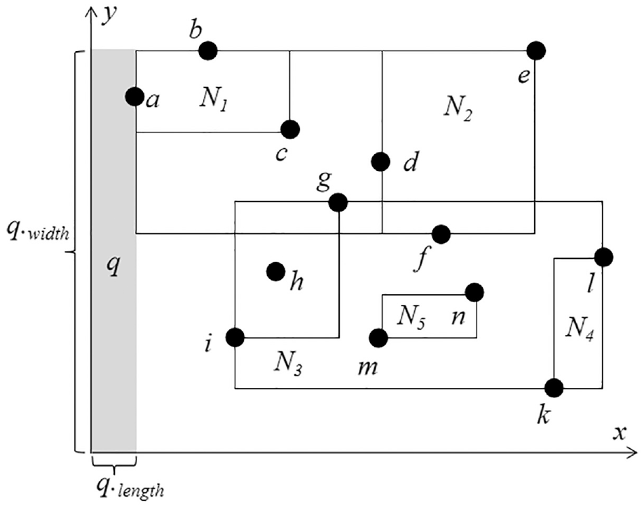
Sliding query window.

Figure 3.

Query process.

This algorithm based on query window reduces the query area by changing the query window constantly and does not need to visit all points in the space, which greatly reduces the number of points to be visited.

Key skyline layers algorithm

The existing methods either compute all the layers³⁷ of the whole data set or needs much comparing computation² for getting the first k layers. Yu et al.³ visit the points concurrently in each dimension, who used binary search and sub-space skyline to investigate each point, and each point needs to be compared with all the points visited by hyperplane, so the computation is much.

According to skyline layer definition, each layer is actually skyline of the data set except all the points in previous layers. Therefore, we propose a new algorithm to compute KSL by visiting less points with less comparison, more importantly, and our algorithm can return multiple layers simultaneously. The detailed procedure is introduced below, and the notations used in algorithm are shown in Table 1.

Table 1.

List of notations.

Notation	Definition
KSL(i)	Set of points in layer_i
MQW	Main query window
MBRS	All of MBR
Mindist_ y	Minimum distance to y axis
Maxdist_ x	Maximal distance to x axis
q_i._visited	Point q_i is visited or not
CQW	Child query window

Our main idea is to create and slide multiple query window (one main window and some children windows) over the points concurrently, to determine which layer the point belongs to for every point visited. We show the detailed process in Algorithm 1. First, all the points are stored in R-Tree, and we initialize KSL(i) = null, each point q_i.visited = false. Second, we construct the main query window (MQW) to find the first point of each layer, the MQW only visits the points not been visited by any query window, we use p_visited to denote whether point p has been visited by any query window (lines 1–4). When a point is visited by MQW, a new child query window (CQW) with this point as its left-top vertex will be born from MQW (lines 6 and 7), and this CQW will slide and visit the points for new layer. When a point e is visited by CQW_i, e_visited is set true to indicate this point has been visited by a query window, then if e.y is the smallest in the points visited by this window, it must belong to layer_i (lines 9–12). The CQWs and MQW continue to slide (lines 13 and 14). The key is that CQW created later must slide after CQW created early, and the MQW is the last one. Each query window is independent, and the points visited by a query window must not be visited by any other query windows, as one point only belongs to one layer. Certainly, the query window created early will stop early too. With these query windows sliding, each layer can be returned, and the lower layer will be returned earlier than the higher ones. When the first point of the kth layer is visited by MQW, this window can stop as we only want to compute the first k layers.

Algorithm 1. Key skyline layers algorithm.
Input: a data set P with 2-dimension space Output: key skyline layers 1 store the points in R-Tree 2 Initialize KSL(1…k) = null, each pointq_i.visited = false; 3 MQW._length = Mindist_y (MBRS) 4 MQW._width = Maxdist_x(MBRS) 5 fori = 1 tokdo 6 if MQW visits pointp&&p._visited = false 7 create CQW_i with p as its left-top vertex 8 while CQW_i._right < MBRS._right 9 check each point e falling in CQW_i 10 sete._visited = true; 11 if pointe._yis the smallest 12 insert e into KSL(i) 13 CQW_icontinues to slide 14 MQW continues to slide 15 return KSL

Algorithm 1. Key skyline layers algorithm.

Input: a data set P with 2-dimension space
Output: key skyline layers
1 store the points in R-Tree
2 Initialize KSL(1…k) = null, each pointq_i.visited = false;
3 MQW._length = Mindist_y (MBRS)
4 MQW._width = Maxdist_x(MBRS)
5 fori = 1 tokdo
6 if MQW visits pointp&&p._visited = false
7 create CQW_i with p as its left-top vertex
8 while CQW_i._right < MBRS._right
9 check each point e falling in CQW_i
10 sete._visited = true;
11 if pointe._yis the smallest
12 insert e into KSL(i)
13 CQW_icontinues to slide
14 MQW continues to slide
15 return KSL

Example

We show an example of Algorithm 1 in Figure 4 based on the data in Figure 1, we aim to compute KSL with k = 3. Figure 4(a) shows the MQW with point p₁ as its right-top, and p₁ is first visited by MQW, so it is inserted into KSL(1), KSL(1) = { p₁}. Then a CQW₁ is born from MQW with p₁ as its left-top, as shown in Figure 4(b), CQW₁ extends to the right until it visits point p₆ which is inserted to KSL(1), KSL(1) = {p₁, p₆}. At the same time, MQW continues to slide the data set after CQW₁.

Figure 4.

Steps of computing skyline layers. (a) KSL = {{p₁}}. (b) KSL = {{p₁, p₆}}. (c) KSL = {{p₁, p₆, p₁₁},{p₃}}. (d) KSL = {{p₁, p₆, p₁₁},{p₃, p₈}}. (e) KSL = {{p₁, p₆, p₁₁},{p₃, p₈, p₁₀},{p₂}}. (f) KSL = {{p₁, p₆, p₁₁},{p₃, p₈, p₁₀},{p₂, p₅}}. (g) KSL = {{p₁, p₆, p₁₁},{p₃, p₈, p₁₀},{p₂, p₅, p₁₂,p₉}}.

Figure 4(c) shows that CQW₁ visits p₁₁ which belongs to KSL(1), and MQW visits p₃ while p_3visited = false, so at this time, CQW₂ is born from MQW with p₃ as its left-top to begin computing KSL(2), KSL(2) = {p₃}. There is an overlap between MQW and CQW₁.

Next, as shown in Figure 4(d), the algorithm updates CQW₁ with p₁₁ as its left-top to continue to slide the data set and updates CQW₂ with p₃ as its left-top. When CQW₂ visits p₈, KSL(2) = {p₃, p₈}, and from now on, there is no point to be visited by CQW₁, so we can conclude KSL(1) = {p₁, p₆, p₁₁}. There is an overlap between CQW₁ and CQW₂.

In Figure 4(e), CQW₂ visits p₁₀, and KSL(2) = {p₃, p₈_,p₁₀}, at the same time, MQW visits p₂ and p_2visited = false, so KSL(3) = {p₂} and CQW₃ will be born. There is an overlap between MQW, CQW₁ and CQW₂.

As shown in Figure 4(f), MQW stops as we only want to compute KSL with k = 3, so MQW needs not to continue, at the same time, three CQWs continue to slide the data set until they reach the right boundary of the rightmost MBR. There is an overlap between CQW₁, CQW₂, and CQW₃. The final result is KSL(1) = {p₁, p₆, p₁₁}, KSL(2) = {p₃, p₈, p₁₀}, and KSL(3) = {p₂, p₅, p₁₂, p₉}. It is worth noting that the order of birth for query windows is CQW₁, CQW ₂ , and CQW₃, and these windows do query in this order too, in other words, the window generated earlier is in the front of queue and MQW is the last one. The final skyline layers are shown in Figure 4(g).

Directed skyline graph optimization

Liu et al.² first proposed the directed skyline graph (DSG) to reflect the domination relationships between points. However, it must compute all the relations between points, and it needs lots of computation as one point should to be compared with all the points in the previous layers even though some relations are transitive or useless. In fact, the useless relationships are unnecessary to compute, and the transitive relationships can be derived by the existing relationships. In this subsection, we propose the new algorithm to optimize DSG construction to make the computing more effective.

Computing DSG for two dimensions

For two dimensional space, we present some properties for DSG which will be used for G-skyline.

Property 2

Given a point p in layer_i and another point q in layer_i ₊ _j, if p does not dominate q, then we can conclude that p._x < q._x and p._y > q._y, or p._x > q._x and p._y < q._y.

Proof

It is obvious and easy to prove. If p does not dominate q, and the layer of p is lower than q, then either p locates at left-top to q, or p locates at rightbottom to q.□

Property 3

Given a point p in layer_i and another point q in layer_i ₊ _j, if p dominates q, then all the parents of p must be q’s parents.

Proof

Point t, as a parent of p, certainly dominates p, so if p dominates q, then t must dominate q.□

Property 4

Assume that all the points in the same layer are sorted by x-coordinate, for a point q in layer_i, the parents of q in the same layer are sequential in point index.

Proof

There are n points sorted in ascending order by x-coordinate in layer_j (j < i), such as p₁, p₂,…, p_n. If p_k and p_m dominate q (k < m), then p_k_.x < q.x, p_k.y < q._y, and p_m.x < q._x, p_m.y < q._y. For any one point p_a (k < a < m) in the same layer, there must be p_a.x < p_m.x and p_a.y < p_k.y, so we can conclude that p_a.x < q._x and p_a.y < q._y, so p_a must dominate q.□

Based on the skyline layers, we compute the DSG from low layer to high layer, and we start at the second layer as the points in layer₁ has no parent. For every point p in layer_i, first it should be compared with the points in layer_i_–1, we should find the maximal index where the point is less than p in x axis, then scan each point in the opposite directions of the x axis, when a point not dominating q is visited, the scan stops and q’s parents in layer_i_–1 are returned (lines 3–6).

In order to find p’s parents in other layers, there is no need to compare p with all the points in each layer. As the DSG is built from low layer to high layer, so when the points in layer_i are checked, DSG has been constructed in precious i–1 layers, we should first find the least parent p_l in layer_i_–2 of the least parent of p in layer_i_–1, and the maximal parent p_m of the maximal parent of p in layer_i_–1, then all the points between p_l and p_m are also p’s parents (lines 8–10). On the other hand, we should visit the points less than p_l and bigger than p_m with index in both two directions until a point not dominating p is visited respectively (lines 11–20).

Do the same computing as above until all the parents of p is found. We can use this method to construct DSG of all the points in the first k layers. In this way, when finding a point’s parents, we need not to compare it with all the points in previous layers. Doing it like this takes full advantage of intermediate result to avoid much redundant computations.

Example

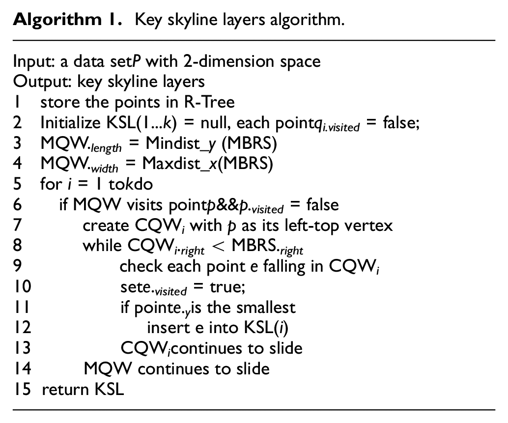
We show an example of Algorithm 2 based on the data in Figure 1(a) and its skyline layers in Figure 4(g). The points in each layer are sorted in ascending order in x axis, such as: p₁, p₆, p₁₁; p₃, p₈, p₁₀; p₂, p₅, p₁₂, p₉. We begin the computation from the second layer. Point p₃ is the first one to be visited, it should be compared with the points in layer₁, we find that the maximal point which is less than p₃ in x axis is p₆, and p₆ can dominate p₃, we get p_3.parent = {p₆}. Then we continue to scan layer₁ in the opposite directions of the x axis, when p₁ is visited, we find that p₁ cannot dominate p₃, so this scan stops. The layer which is lower than layer₂ is only layer₁, so we can get p_3.parent = {p₆}. We use the same method to get p_8.parent = {p₁₁}, p_10.parent = {p₁₁}. In layer₃, for point p₂, we should compare it with the points in layer₂ first, we find the maximal point which is less than p₂ in x axis is p8, the minimum point is p3, we can get p2._parent = {p₃, p₈} in layer₂, then we continue to find p₂_’s parents in layer₁. The minimal parent of p₃ is p₆, and the maximal parent of p₈ is p₁₁, so the points between p₆ and p₈ in layer₁ are also p₂_’s parents. Then we continue to visit points with index larger than p₁₁ and the points with index smaller than p₆, but there is no p₂_’s parent any more. So we can get p_2.parent = {p₈, p₁₁, p₃, p₆}. We use the same method to get _p5.parent = {p₈, p₁₁, p₆}, p_12.parent = {p₈, p₁₁}, and _p9.parent = {p₁₀, p₁₁}. The final DSG is shown in Figure 5. We can see that our method can take full advantage of intermediate result about point’s parents and greatly reduces the amount of computation.

Algorithm 2. Computing DSG in 2-dimension space.
Input: k skyline layers of data setP Output: DSG ofP The points in the same layer are sorted in ascending order inxaxis. 1 fori = 2 tok 2 { for each pointpinlayer_i 3 { Initializep._parent = NULL; 4 find p’s parentp_mwith maximal index inlayer_i_–₁ 5 find p’s parentp_lwith minimum index inlayer_i_–₁ 6 move points betweenp_landp_mtop._parent 7 forj = i–1 to 1 8 {p_m = p_m’s parent with maximal index inlayer_j 9p_l = p_l’s parent with minimum index inlayer_j 10 move points betweenp_landpmtop._parent 11 x = m + 1; 12 while(p_x≺p) 13 { movep_xtop._parent; 14 x ++;} 15 p_m = p_x_–₁; 16 t = l–1; 17 while(p_tp) 18 { movep_ttop._parent; 19 t- -;} 20 p_l = p_t + 1; } } 21 Return DSG

Algorithm 2. Computing DSG in 2-dimension space.

Input: k skyline layers of data setP
Output: DSG ofP
The points in the same layer are sorted in ascending order inxaxis.
1 fori = 2 tok
2 { for each pointpinlayer_i
3 { Initializep._parent = NULL;
4 find p’s parentp_mwith maximal index inlayer_i_–₁
5 find p’s parentp_lwith minimum index inlayer_i_–₁
6 move points betweenp_landp_mtop._parent
7 forj = i–1 to 1
8 {p_m = p_m’s parent with maximal index inlayer_j
9p_l = p_l’s parent with minimum index inlayer_j
10 move points betweenp_landpmtop._parent
11 x = m + 1;
12 while(p_x≺p)
13 { movep_xtop._parent;
14 x ++;}
15 p_m = p_x_–₁;
16 t = l–1;
17 while(p_tp)
18 { movep_ttop._parent;
19 t- -;}
20 p_l = p_t + 1;
}
}
21 Return DSG

Figure 5.

DSG.

High-dimensional space

For the data set with higher dimensional space, we can use a method similar to Algorithm 2 to compute DSG. The points are visited from layer₂ to higher layers one by one. For each point p to be computed in layer_i, we should compare it with points from layer_i_–1 to layer₁. For the points in layer_j(1 ≦ j < i), some parents can be returned directly by transitive relation, then the points except these parents are sorted by x-coordinate in ascending order, the points in front of p are selected to form a set D₁, then all the points in D₁ are sorted by y-coordinate in ascending, the points in front of p are selected to form a set D₂, and then doing it like that in another dimension until D_d is returned where d is dimension size of the data set, and all the points in D_d are the parents of p. Similar to the Algorithm 2, as the DSG with first i–1 layers has been constructed, so when layer_j is visited, the points which are already p’s parents by transitivity are no longer involved in the calculation.

Computing G-skyline groups

In this section, we present a new algorithm to compute G-skyline efficiently based on properties and methods above. First, we give some theorems and definitions.

Primary points

Theorem 4

A point in a G-skyline group cannot be dominated by a point outside this group.²

Theorem 5

Given a point p, if p is in a G-skyline group, p’s parents must be included in this G-skyline group.²

Theorem 6

As a G-skyline group c, it must satisfy one of two conditions: the points in c are either all traditional skyline points, or some are traditional skyline points and others are not, but for each point of these others in c, it must be dominated by some traditional skyline points in c and it cannot be dominated by any point outside c.

Proof

Given a G-skyline group c = {p₁, p₂,…, p_n, q₁, q₂,…, q_m}. If each point of c is traditional skyline point, we cannot find another point dominating it, so there is no group with same size can g-dominate group c; therefore, group c is G-skyline group according to definition 4. If p₁, p₂,…, p_i are traditional skyline points and q₁, q₂,…, q_x (x≦m) are not, according to Theorem 5, we get that for each point q_j (1 ≦ j ≦ x), its parents must be in group c, and it will be dominated by at least one traditional point, and according to Theorem 4, it cannot be dominated by any point outside c. Any group not satisfying one of above conditions must not be G-skyline group.

For any other groups, there are other two kinds conditions: there is no traditional point in c, or c consist of some traditional skyline points and some other points whose parents are not in c. If a group satisfies one of these two conditions, we can easily find another group g-dominating it, and this group must not be G-skyline group.

Each G-skyline group consists of points in the first k layers, but these points are not evenly distributed across these k layers. In fact, the traditional skyline points have stronger domination and they play vital important in G-skyline.

Definition 8 (Primary points)

For G-skyline, the points in layer₁ are primary points. According to Theorem 6, each G-skyline group must contain at least one point in layer₁.

Definition 9 (Secondary points)

The points in G-skyline groups which are not primary points are secondary points.

Lemma 1

The higher the layer, the less role the data points in that layer play in computing the G-Skyline.

Proof

This lemma is easy to prove. When the layer is higher, the points in this layer will have less dominant power, and the number of points dominated by which will be less. For a G-skyline group, the point in which and all its parents are must in this group, so if a point has less dominant power, there is less chance for it to be in a G-skyline group, so this kind of point will play less role in computing G-skyline.□

Example

We use a synthetic data set containing 1000 points with three-dimensional space to show the proportion of primary point and secondary point in the G-skyline groups. When k = 3, there are 68 points in layer₁, 126 points in layer₂, 163 points in layer₃, and 69,246 G-skyline groups. The number of times the primary points and the secondary points appear in G-skyline are respectively 197,975 and 9763. We find that the proportion of occurrences of primary points is 197,975/(197,975 + 9763) ≈ 95.3%, and the proportion of occurrences of the points in layer₂ is about 4%, the proportion of occurrences of the points in layer₃ is about 1%.

Table 2 shows the proportion of primary points in G-skyline on different data set with varying parameters, while data set size is 1000. From the statistical data we find that the proportion of primary points occurrence in G-skyline groups is very high, up to 90% most time. We can infer the conclusion: primary points play an important role in formation of G-skyline groups.

Table 2.

Percentage of primary points.

Data set	d	k
Data set	d	2	3	4	5	6
Correlateddata set	2	81.6	42.6	18.7	9.2	7.6
	3	93.1	90.4	90.6	86.7	82.1
	4	99.3	94.8	96.2	95.3	93.2
	5	99.7	99.6	98.4	98.1	95.8
Independentdata set	2	94.8	86.4	37.3	29.4	32.6
	3	98.3	95.3	91.2	91.6	90.4
	4	99.5	98.6	96.9	95.8	94.3
	5	99.8	99.5	99.8	99.2	99.6
Anti-correlateddata set	2	99.8	94.6	92.7	91.6	87.2
	3	99.9	97.8	97.6	96.5	93.7
	4	99.9	99.8	99.3	99.6	98.6
	5	99.9	99.9	99.8	99.9	99.3

The primary points in layer₁ have higher dominant power, the groups including some of them can dominate many groups composed by points in other layers based on above theorems. We find it is crucial and necessary to enumerate the groups composed by all primary points and propose a method to compute groups extended by primary points. On the contrary, the number of secondary points is relatively small, although it increases slightly with k increasing, these secondary points play a minor role in computing G-skyline groups all the time. That is to say, most groups composed by points in higher layers are useless for G-skyline and should be filtered directly.

Based on above motivations, we propose a new algorithm computing G-skyline groups directly by extending primary points according to our rules instead of visiting a large groups consist of lots of useless groups, and our algorithm needs not compute G-skyline (k) from G-skyline(k–1) recursively.

Highly-efficient method for G-skyline

In this subsection, we propose a highly effective algorithm to compute G-skyline. As the primary points play vital role in G-skyline groups, first, we enumerate all the groups composed of points in layer1, then each group is extended by adding its eligible children in next layer. For each candidate group G, we should test its every point to find eligible children in next layer, then enumerate these children and combine each enumeration with group G to construct new candidate group. How to find the eligible children to be combined with group G? Each eligible child p must satisfy—p._parent|< k and all of p’s parents are in group G. If—p._parent| ≧ k, we can prune p and its children directly according to Rule 1. How to enumerate the combinations consist of G’s children? Based on the eligible children, we enumerate all combinations with size not larger than k–|G,| and combine these combinations with G respectively. Thus, we check and extend each candidate group in the same way until we get all the G-skyline groups.

Besides the previous definitions and theorems, we present the key rules to be used in computing G-skyline groups.

Rule 1

We use p._parent to denote all parents of point p. If—p._parent—≥ k–1, the children of p can be pruned.

Proof

If—p._parent—≥ k–1, that is to say, for any child q of p, there must be—q._parent—≥ k. For any group containing point q with size k, it cannot contain all parents of q, so according to Theorem 5, we can conclude that q must not be in G-skyline group.□

Rule 2

For each point p in layer_i, if—p._parent_|≥ k–1, we should not check any other points in layer_j where j > i.

Proof

From Rule 1, we find that if|p._parent| ≥ k–1, the children of p can be pruned, so if this condition is suitable for all points in layer_i, we should not visit the points in higher layer_j (j > i), and these points can be pruned directly.□

First, we should enumerate all the groups composing of primary points with group size not larger than k, and use symbol S to represent these groups (line 1). We use these groups as the starting for computing G-skyline. For each group gi in S, if it is G-skyline group with size k, it can be output directly (lines 3 and 4), or we will check if it has eligible children. For each point q of group gi, we should find all its children in next layer, and store these children in a set C (lines 6 and 7), then we check whether each point in C is eligible point. For a point p in C, if|p._parent|> k–1, it and its children can be pruned directly according to Rule 1 (lines 9 and 10), else if p’s parents are not all in C, it is not suitable to be combined with group g_i according to Theorem 5 (lines 11 and 12). After doing it like this, if C is not null, then we enumerate all the combinations with size not bigger than k–|G,| then combine each with g_i to construct new candidate group inserted into S (lines 13–16).

Example

Figure 6 shows an example of Algorithm 3 to compute G-skyline(3) based on the data set in Figure 1. Figure 6(a) shows the DSG of data set with solid arrow indicating dominant relationship, and each point has a tag to indicate the number of its parents. In Figure 6(b), the symbol “—” means stop, and the symbol “√” means the group is a G-skyline group.

Figure 6.

An example to find G-skyline when k = 3: (a) DSG and (b) G-skyline.

Algorithm 3. Fast computing G-skyline.
Input: a DSG Output: G-skyline( k ) 1 enumerate all groups by points in layer1 to construct a queue S ; 2 for each group g_i in S do 3 { if gi is G-skyline group with size k 4 output g_i ; 5 else 6 { for each point q in g_i 7 find q ’s children in next layer → C ; 8 for each p in C 9 { if\| p._parent \| > k –1 then 10 prune p and its children; 11 else if p ’s parents are not all in C then 12 remove p from C ; } 13 if C is not null 14 { enumerate all groups as Q by points in C ; 15 combine each groups in Q and gi as g ; 16 put g into S ; } } } 17 return G-skyline( k );

Algorithm 3. Fast computing G-skyline.

Input: a DSG
Output: G-skyline( k )
1 enumerate all groups by points in layer1 to construct a queue S ;
2 for each group g_i in S do
3 { if gi is G-skyline group with size k
4 output g_i ;
5 else
6 { for each point q in g_i
7 find q ’s children in next layer → C ;
8 for each p in C
9 { if| p._parent | > k –1 then
10 prune p and its children;
11 else if p ’s parents are not all in C then
12 remove p from C ;
}
13 if C is not null
14 { enumerate all groups as Q by points in C ;
15 combine each groups in Q and gi as g ;
16 put g into S ;
}
}
}
17 return G-skyline( k );

First, All points in layer₁ are enumerated to output groups which are basic to compute G-skyline, these groups are {p₁}, {p₆}, {p₁₁}, {p₁, p₆}, {p₁, p₁₁}, {p₁₁, p₆} and {p₁, p₆, p₁₁}. Next, we will check each group to output G-skyline groups, or combine it with some of their children groups.

For group {p₁}, it has no child, so it does not need to be extended.

For group {p₁₁}, the layer of its single point is layer₁, it has two children p₈ and p₁₀ in layer₂, because|p_8.parent| and|p_10.parent| are both smaller than 3, and their single parent is in group {p₁₁}, so we enumerate and combine these two children with group {p₁₁}, then get three groups {p₁₁, p₈}, {p₁₁, p₁₀} and {p₁₁, p₁₀, p₈}. Obviously, {p₁₁, p₁₀, p₈} is a G-skyline(3) group. Point p₈ has three children, but only p₁₂_’s parents are all in group {p₁₁, p₈} and|p_12.parent| = 2 < 3, while|p_5.parent| = 3 and|p_2.parent| = 4 > 3, so only p₁₂ can be combined with {p₁₁, p₈} to construct new G-skyline group {p₁₁, p₈, p₁₂}. Doing it like this, we can get a G-skyline group {p₁₁, p₁₀, p₉} by combine {p₁₁, p₁₀} with p₉ which is p₁₀_’s single child.

Such as group {p₁₁, p₆}, two points are in the same layer1, so we only consider their children in layer₂. In layer₂, we find the child of p₆ is p₃, and the children of p₁₁ are p₈ and p₁₀. Point p₃ with|p_3.parent|< 3 can be combined with group {p₁₁, p₆} to construct {p₁₁, p₆, p₃} as its parent is only p₆ and p₆ is in this group, so this new group is a G-skyline(3) group. Similarly, p₈_’s parent and p₁₀_’s parent are only p₁₁, so p₈ and p₁₀ can be separately combined with group {p₁₁, p₆} to construct {p₁₁, p₆, p₈} and {p₁₁, p₆, p₁₀}, and these new groups are also G-skyline(3) groups.

Other original groups are processed in the same way, and the final result is shown in Figure 6(b), and each G-skyline group is marked by tick. In this way, we can quickly compute G-skyline groups gradually.

Experiments

In this section, we show the experimental test on our methods in efficiency and correctness. The test programs are written in Java, and run in a PC with Intel Core i7 processors, 512G SSD and 16G RAM. The synthetic data set and real sensor data set are used in the process of experiment.

Experiment preparation

In order to test and evaluate the algorithms in different aspects, and keep the universality of algorithms, we adopt synthetic data set and real-world sensor data set, respectively, to test our algorithms.

After the skyline query was proposed and the experiments were carried out based on three different kinds of synthetic data set,¹ most of experiments about subsequent skyline query algorithms are also carried out based on these three kinds of data set. So in our experiments, to test the processing effect of the algorithm on different types of data, three kinds of synthetic data sets are generated¹ for experiments: the correlated data set (COR), the independent data set (IND) and the anti-correlated data set (ANTI-COR). The examples of three kinds of synthetic data set with two dimensions are shown in Figure 7. We can find that their distributions are different from each other: the two coordinates of the correlated points have the same variation trend, and this kind of points which are good in one dimension are also good in other dimension; while the two coordinates of the anti-correlated points have the opposite variation trend, and this kind of points which are good in one dimension are bad in other dimension; however, the two coordinates of the independent points have no relation in the variation trend. For the correlated data set and the anti-correlated data set, the points are generated by selecting a plane perpendicular to the line from (0,…, 0) to (1,…, 1) using a normal distribution, while for the independent data set, all attribute values of points are generated independently using a uniform distribution. The real-world sensor data set is obtained from a forest environment monitoring project, which includes temperature, humidity, daily rainfall, daily evaporation and daily temperature range. In order to ensure the stability of the experimental results, each experiment is repeated 100 times and the average value is used as the final result.

Figure 7.

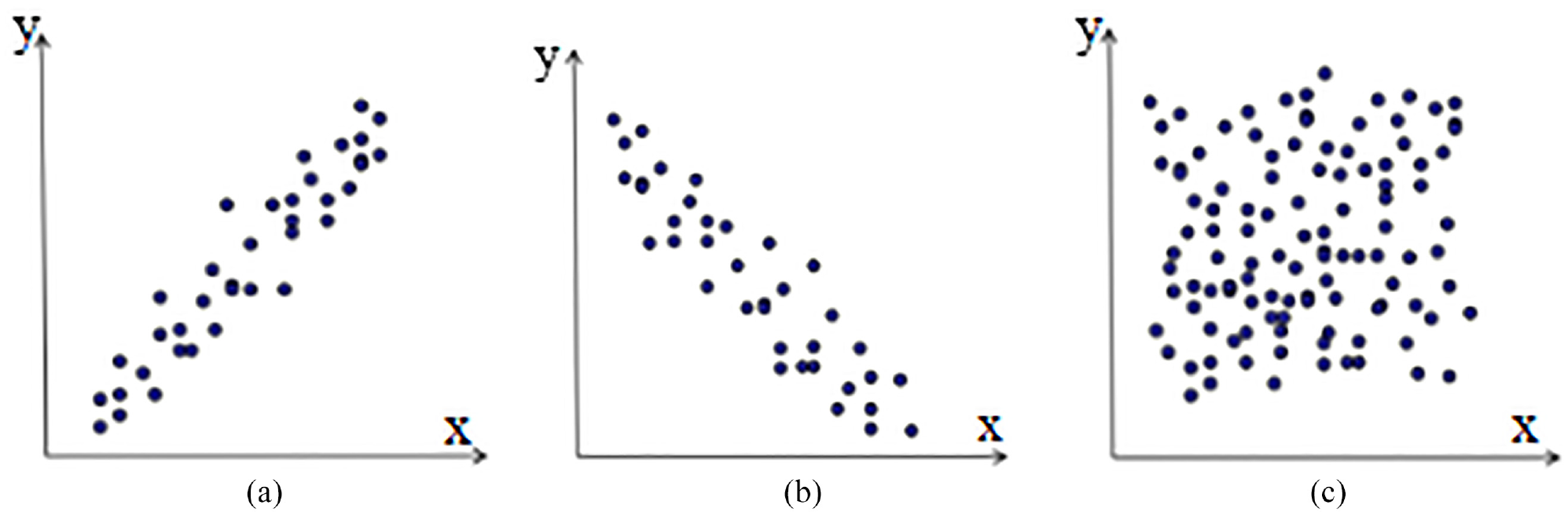
Example of synthetic data set: (a) COR, (b) ANTI-COR, and (C) IND.

In order to compare our algorithms with other existing algorithms presented in recent years, we select point-wise algorithm (PWA) and fast pwise algorithm (FPA) to participate in the comparison, as PWA is the first G-skyline query algorithm and FPA is the improvement based on PWA. Although FPA can prune the edge for DSG to make the algorithm more effective than PWA, it need much time to find each G-skyline groups by comparison yet. Our algorithm not only optimize the skyline layers and DSG computing, but also present a new method to find G-skyline groups directly based on skyline layers and DSG. We choose these two algorithms to compare with our algorithm in order to find out the superiority of our algorithm in execution efficiency. The algorithms to be tested in the experiments are as follows.

KSL: The algorithm to compute key skyline layer for a data set in this article.

FCG: Fast computing G-skyline algorithm proposed in our article.

PWA: Point-wise algorithm for G-skyline in article.²

FPA: Fast pwise algorithm to compute G-skyline in article.³ In fact, there are two algorithms FPA and FUA in article³ to compute G-skylines in different way, but FPA is better than FUA in most of time, so we chose FPA for comparison.

Key skyline layers on synthetic data

In this subsection, we test the methods for computing key skyline layers on synthetic data set. Figures 8 –10 show the running time cost of computing key skyline layers by algorithm PWA, FPA and KSL.

Figure 8.

Computing key skyline layers with different k: (a) COR, (b) IND, and (C) ANTI-COR.

Figure 9.

Computing key skyline layers with different n: (a) COR, (b) IND, and (C) ANTI-COR.

Figure 10.

Computing key skyline layers with different d: (a) COR, (b) IND, and (C) ANTI-COR.

Figure 8 shows the running time cost for computing key skyline layers by each method with varying group size k (n = 1000, d = 2). We find that the running time of PWA and FPA is bigger than KSL especially when the group size varies from 6 to 14; however, when k is not big (Figure 8, k = 2 and k = 4), there are not many points in first k layers, our method is not much faster than other two methods. But our method performs better with group size k increasing, as some query windows are working at the same time.

Figure 9 shows the time cost of computing key skyline layers by each method with varying data set size n (k = 6, d = 2). We find that the running time of these methods increases very fast with n increasing, the time growth trend is close to linear growth, as the amount of computation is closely related to the amount of data set. However, when n is larger than 10⁴, our method performs much better than others as the query windows are smaller and smaller, so the number growth of points to be visited is slowing down.

Figure 10 shows the time cost of computing key skyline layers by each method with varying dimension size d (n = 10000, k = 4). We find that PWA and FPA algorithms needs much time with d increasing, the reason is that each point should be compared with all existing points in PWA, while FPA wastes some time to update the sub-space skyline. The chance for one point dominating another point will be smaller with d increasing, and the points in the first k layers will be more with d increasing, so each method will need much time. However, our method performs better than other two, as it can visit different layers by some query windows at the same time.

G-skyline on synthetic data

In this section, we show the experimental results of methods for computing G-skyline based on different synthetic data set. As the time cost of computing skyline layers is shown in 6.2, we only record the time cost except skyline layers time cost to compare the efficiency of methods for finding and outputting G-skyline groups.

Figure 11 shows the time cost and output size of three methods to compute G-skyline groups with varying data set size n (d = 2, k = 3). We find that the time cost increases faster and faster from COR data set, IND data set to ANTI-COR data set, the reason is that there will be much points in the first k layers for ANTI-COR data set, so the computation will be larger than other two data sets. The output size increases about linearly with the increasing of n.

Figure 11.

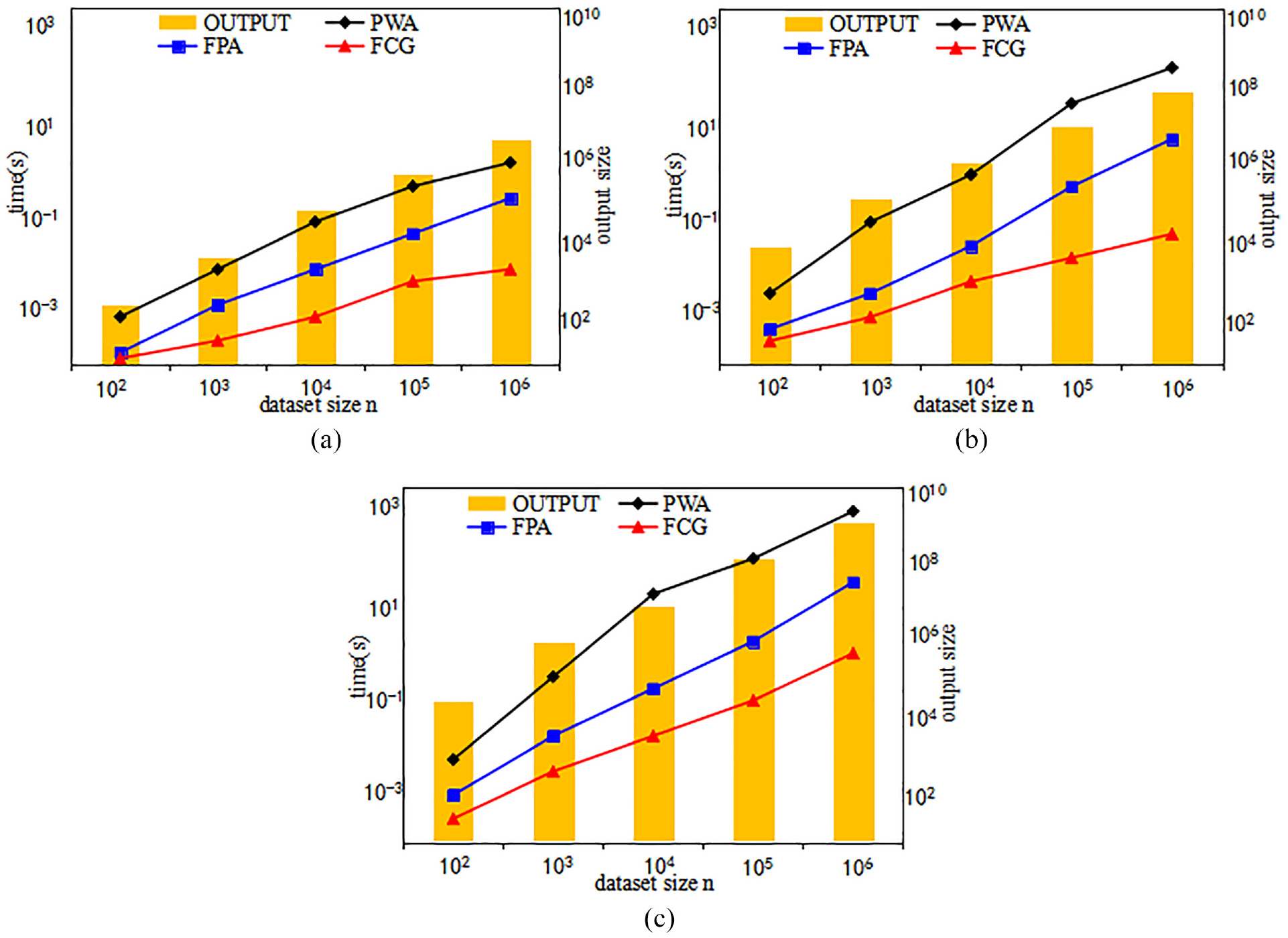
Computing G-skyline with different n: (a) COR, (b) IND, and (C) ANTI-COR.

Figure 12 shows the time cost and output size of three methods to compute G-skyline groups with varying group size k (d = 2, n = 10000). We find that the time cost is greatly influenced by varying k, as there will be more points to be computed with k increasing, at the same time, we find the output size increases fast with k increasing. However, our algorithm performs better, as our filtering policy is efficient to prune more useless data as early as possible.

Figure 12.

Computing G-skyline with different k: (a) COR, (b) IND, and (C) ANTI-COR.

Figure 13 shows the time cost and output size of three methods to compute G-skyline groups with varying dimension size d (k = 3, n = 10000). We find that the time cost increases fast with d increasing, as the number of points in the first k layers will be more and more with d increasing, and the number of groups to be tested will be more accordingly. However, the growth rate of the time cost tends to slow down when d is larger than 6 approximately, as the most points locate in the first k layers when d increases, so even if d continues to increase, the number of points in the first k layers increases slowly.

Figure 13.

Computing G-skyline with different d: (a) COR, (b) IND, and (C) ANTI-COR.

Key skyline layers on real sensor data

After all, experiments on synthetic data cannot reflect the processing effect in practical application environment. In this subsection, we do experiments on real sensor data to show the effect of processing real data by algorithms, the experiment results are shown in Figure 14.

Figure 14.

Computing skyline layers with different parameters: (a) group size k, (b) data set size n, and (c) dimension size d.

Figure 14(a) shows the result of computing key skyline layers with varying group size k(n = 1000, d = 5), we find that k has obvious influence on the algorithm as the points increase a lot with k increasing while our algorithm performs better than other two methods. Figure 14(b) shows the impact of varying data set size n (k = 3, d = 5) on methods. The change of n does not have much effect on the time cost of methods. The time cost of methods with varying dimension size d(k = 6, n = 2000) is shown in Figure 14(c), they are influenced by d obviously due to most of points in the first k layers with d increasing.

G-skyline on real sensor data

In this subsection, the algorithms for computing G-skyline are implemented on real sensor data set and the result are shown in Figure 15.

Figure 15.

Computing G-skylines with different parameters: (a) group size k, (b) data set size n, and (C) dimension size d.

Figure 15(a) shows the time cost for computing G-skyline with varying group size k(d = 5, n = 1000) and the output size. We find that the output size increase smoothly, but the time cost increase quickly with k increasing, the reason maybe that when k increases, there will be more points to be tested. It is worth noting that FCG algorithm is much better than other algorithms PWA and FPA, the reason maybe that the number of points in each layer is similar, so each query window will spend less time to visit points.

Figure 15(b) shows the time cost for computing G-skyline with varying data set size n (d = 5, k = 4) and the output size. An interesting phenomenon is that there is no significant fluctuation in the time cost and output size, and the values of these two parameters are big, the reason maybe that real sensor data set is anti-correlated, so many points locates in first k layers and the number of these points will not change much.

Figure 15(c) shows the time cost for computing G-skyline with varying dimension size d (k = 3, n = 1000) and the output size. We find that the time cost and output size both increase obviously with d increasing, the reason is that point’s domination ability will be weaker when dimension size is big, so more points will locate in the first k layers, and the computation complexity and the output size become bigger accordingly.

Conclusion and future work

In this article, we focused on the problem of finding G-Skyline groups over the data set in the WSN. In order to compute the G-Skyline groups efficiently, we presented a method based on multiple query windows to compute key skyline layers quickly. Then we optimize the DSG method by omitting most computation between the point and its parents in previous layer. Finally, we proved the primary points’ importance for G-skyline and proposed new method to compute G-skyline groups from the enumeration groups of primary points efficiently. The experiment results based on the synthetic data and real data show that our algorithms perform better than others. In the future, we will consider how to compute the G-Skyline groups based on data dispersion analysis in wireless network.

Footnotes

Acknowledgements

The authors thank all the members in database laboratory of Baicheng Normal University and Donghua University.

Handling Editor: Peio Lopez Iturri

Declaration of conflicting interests

The author(s) declared no potential conflicts of interest with respect to the research, authorship, and/or publication of this article.

Funding

The author(s) disclosed receipt of the following financial support for the research, authorship, and/or publication of this article: This research was funded by Scientific Research Project of Jilin Province (grant nos. JJKH20210005KJ, JJKH20190621KJ, and JJKH20210012KJ), China; Natural Science Foundation of Heilongjiang Province (grant no. LH2019F039), China.

ORCID iD

Leigang Dong

References

Borzsonyi

Kossmann

Stocker

. The skyline operator. In: Proceedings of the ICDE conference, 2001, pp.421–430, http://www.cs.ucr.edu/~ravi/CS236Papers/skyline-operator.pdf

Liu

Xiong

Pei

, et al. Finding Pareto optimal groups: group-based skyline. In: Proceedings of the VLDB endowment, 2015, pp.2086–2097, http://www.vldb.org/pvldb/vol8/p2086-liu.pdf

Qin

Liu

, et al. Fast algorithms for Pareto optimal group-based skyline. In: Proceedings of the CIKM conference, 2017, pp.417–426, http://www.mathcs.emory.edu/aims/pub/yu17cikm.pdf

Zhu

, et al. Computing skyline groups: an experimental evaluation. In: Proceedings of the ACM Turing celebration conference, Chengdu, China, 17–19 May 2019. New York: ACM.

Chomicki

Godfrey

Gryz

, et al. Skyline with presorting. In: Proceedings of the ICDE conference, Bangalore, India, 5–8 March 2003, pp.717–719. New York: IEEE.

Tan

Eng

Ooi

Efficient progressive skyline computation. In: Proceedings of the VLDB conference, 2001, pp.301–310, http://www.vldb.org/conf/2001/P301.pdf

Kossmann

Ramsak

Rost

. Shooting stars in the sky: an online algorithm for skyline queries. In: Proceedings of the VLDB conference, 2002, pp.275–286, http://www.vldb.org/conf/2002/S09P01.pdf

Liu

Algorithm for skyline queries based on window query. J Yanshan Univ 2005; 5: 398–402.

Lee

Hwang

SW.

Toward efficient multidimensional subspace skyline computation. VLDB J 2014; 23(1): 129–145.

10.

Jiang

Zhang

Lin

, et al. Efficient column-oriented processing for mutual subspace skyline queries. Soft Comput 2020; 24(1): 15427–15445.

11.

Dong

, et al. Efficient subspace skyline query based on user preference using MapReduce. Ad Hoc Netw 2015; 35: 105–115.

12.

Chan

Jagadish

Tan

, et al. Finding k-dominant skylines in high dimensional space. In: Proceedings of the SIGMOD conference, 2006, pp.503–514, http://dbgroup.eecs.umich.edu/files/k_dominant.pdf

13.

Miao

Gao

Chen

, et al. k-dominant skyline queries on incomplete data. Inform Sci 2016; 367–368: 990–1011.

14.

Lee

You

Hwang

Personalized top-k skyline queries in high-dimensional space. Inform Syst 2009; 34(1): 45–61.

15.

Jiang

Zhang

Lin

, et al. Incremental evaluation of top-k combinatorial metric skyline query. Knowl Based Syst 2015; 74: 89–105.

16.

Attique

Afzal

Ali

, et al. Geo-social top-k and skyline keyword queries on road networks. Sensors 2020; 20(3): 798.

17.

Jiang

Zhang

Gao

, et al. Efficient top k query processing on mutual skyline. J Comput Res Develop 2013; 50(5): 986–997 (in Chinese).

18.

Son

Stehn

Knauer

, et al. Top-k Manhattan spatial skyline queries. Inform Process Lett 2017; 123(1): 27–35.

19.

Kim

Lee

Kim

MH.

Simultaneous processing of multi-skyline queries with MapReduce. IEICE Trans Inform Syst 2017; E100-D: 7.

20.

Zaman

Siddique

Annisa

, et al. Finding key persons on social media by using MapReduce skyline. Int J Netw Comput 2017; 7(1): 86–104.

21.

TMN

Cao

Answering skyline queries on probabilistic data using the dominance of probabilistic skyline tuples. Inform Sci 2016; 340–341: 58–85.

22.

Pei

Jiang

Lin

, et al. Probabilistic skylines on uncertain data. In: Proceedings of the VLDB conference, 2007, pp.15–26, https://www2.cs.sfu.ca/~jpei/publications/probskyline-vldb07.pdf#:~:text=Computing%20a%20probabilistic%20skyline%20is%20much%20more%20compli-cated, are%20tens%20of%20timesfaster%20than%20 the%20straightforward%20method.

23.

Pujari

Kagita

Garg

, et al. Efficient computation for probabilistic skyline over uncertain preferences. Inform Sci 2015; 324: 146–162.

24.

Ren

Lian

Ghazinour

Skyline queries over incomplete data streams. VLDB J 2019; 28(12): 961–985.

25.

Liu

Ren

, et al. Parallelizing uncertain skyline computation against n-of-N data streaming model. Concurr Comput Pract Exp 2019; 31(4): e4848.1–e4848.20.

26.

Yoo

. An efficient scheme for continuous skyline query processing over dynamic data set. In: Proceedings of the international conference on big data and smart computing, Bangkok, Thailand, 15–17 January 2014, pp.54–59. New York: IEEE.

27.

Matteis

Girolamo

Mencagli

A multicore parallelization of continuous skyline queries on data streams. In: Träff

Hunold

Versaci

(eds) Euro-Par 2015: parallel processing: lecture notes in computer science (LNCS), vol. 9233. Berlin: Springer, 2015, pp.402–413.

28.

Zhu

JX.

Skyline cohesive group queries in large road-social networks. In: Proceedings of the ICDE conference, Dallas, TX, 20–24 April 2020. New York: IEEE.

29.

Yin

Zhou

Zhang

, et al. On efficient processing of continuous reverse skyline queries in wireless sensor networks. KSII Trans Intern Inform Syst 2017; 11(4): 1931–1953.

30.

Wang

Song

Wang

, et al. Geometry-based distributed spatial skyline queries in wireless sensor networks. Sensors 2016; 16(4): 454.

31.

Ahmed

Nafi

Gregory

Enhanced distributed dynamic skyline query for wireless sensor networks. J Sens Actuat Netw 2016; 5(1): 2.

32.

Wang

Xin

Wang

Alternative tuples based probabilistic skyline query processing in wireless sensor networks. Math Probl Eng 2015; 2015: 813507.

33.

Chung

Lee

Top-k combinatorial skyline queries. In: Proceedings of the 15th international conference on database systems for advanced applications (DASFAA 2010), Jeju, Republic of Korea, 24–27 September 2010. Berlin: Springer.

34.

Zhu

Liu

, et al. Top-k dominating queries on skyline groups. IEEE Trans Knowl Data Eng 2020; 32(7): 1431–1444.

35.

Yang

Zhou

, et al. Efficient processing of top k group skyline queries. Knowl Based Syst 2019; 182: 104795.1–104795.12.

36.

Zhou

Yang

, et al. Efficient approaches to k representative G-skyline queries. ACM Trans Knowl Discov Data 2020; 14(5): 1–27.

37.

Park

Group skyline computation. Inform Sci 2012; 188: 151–169.

38.

Zhang

Hassan

, et al. On skyline groups. IEEE Trans Knowl Data Eng 2014; 26(4): 942–956.

39.

Chung

Lee

Efficient computation of combinatorial skyline queries. Inform Syst 2013; 38: 369–387.

40.

Guo

Wulamu

, et al. Efficient processing of skyline group queries over a data stream. Tsinghua Sci Technol 2016; 21(1): 29–39.

41.

Dong

Liu

Cui

, et al. G-skyline query over data stream in wireless sensor network. Wirel Netw 2020; 26: 129–144.

42.

Guttman

. R Trees: a dynamic index structure for spatial searching. In: Proceedings of the annual meeting (SIGMOD’84), Boston, MA, 18–21 June 1984. Cham: Springer.

Efficiently computing Pareto optimal G-skyline query in wireless sensor network

Abstract

Keywords

Introduction

Motivation

Contributions

Organization

Related works

Key skyline layers

Definitions and theorems

Definition 1 (dominate)

Definition 2 (skyline)

Definition 3 (g-dominante)

Definition 4 (G-skyline)

Example 1

Definition 5 (skyline layers)

Theorem 1

Theorem 2

Theorem 3

Computing key skyline layers

Definition 6 (key skyline layers)

Definition 7 (dominant region)

Property 1

Proof

Basic algorithm for layer

Key skyline layers algorithm

Example

Directed skyline graph optimization

Computing DSG for two dimensions

Property 2

Proof

Property 3

Proof

Property 4

Proof

Example

High-dimensional space

Computing G-skyline groups

Primary points

Theorem 4

Theorem 5

Theorem 6

Proof

Definition 8 (Primary points)

Definition 9 (Secondary points)

Lemma 1

Proof

Example

Highly-efficient method for G-skyline

Rule 1

Proof

Rule 2

Proof

Example

Experiments

Experiment preparation

Key skyline layers on synthetic data

G-skyline on synthetic data

Key skyline layers on real sensor data

G-skyline on real sensor data

Conclusion and future work

Footnotes

Acknowledgements

Declaration of conflicting interests

Funding

ORCID iD

References